Super-Consistent Estimation of Points of Impact in Nonparametric Regression with Functional Predictors
Dominik Po{\ss}, Dominik Liebl, Alois Kneip, Hedwig Eisenbarth, Tor D., Wager, Lisa Feldman Barrett

TL;DR
This paper introduces a super-consistent estimator for identifying specific impactful points in functional predictors within nonparametric regression models, improving accuracy without prior knowledge of model components.
Contribution
The authors develop a novel estimator for points of impact that achieves super-consistent convergence and does not require pre-estimates of other model parts.
Findings
Estimator has super-consistent convergence rate
Method performs well in finite samples
Applicable to nonparametric and generalized linear models
Abstract
Predicting scalar outcomes using functional predictors is a classic problem in functional data analysis. In many applications, however, only specific locations or time-points of the functional predictors have an impact on the outcome. Such ``points of impact'' are typically unknown and have to be estimated in addition to estimating the usual model components. We show that our points of impact estimator enjoys a super-consistent convergence rate and does not require knowledge or pre-estimates of the unknown model components. This remarkable result facilitates the subsequent estimation of the remaining model components as shown in the theoretical part, where we consider the case of nonparametric models and the practically relevant case of generalized linear models. The finite sample properties of our estimators are assessed by means of a simulation study. Our methodology is motivated by…
Click any figure to enlarge with its caption.
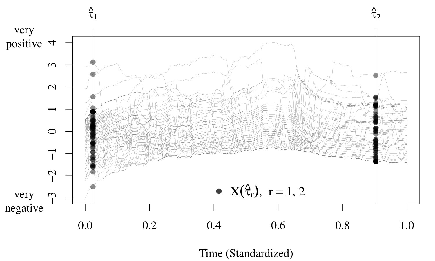 Figure 1
 Figure 2
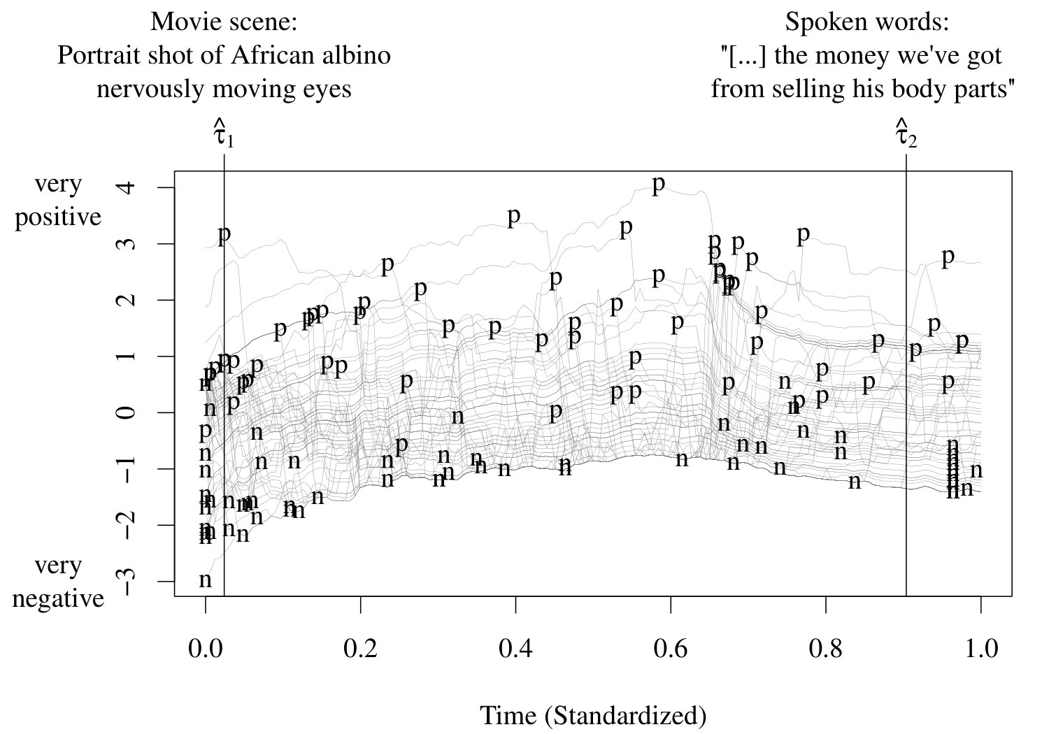 Figure 3
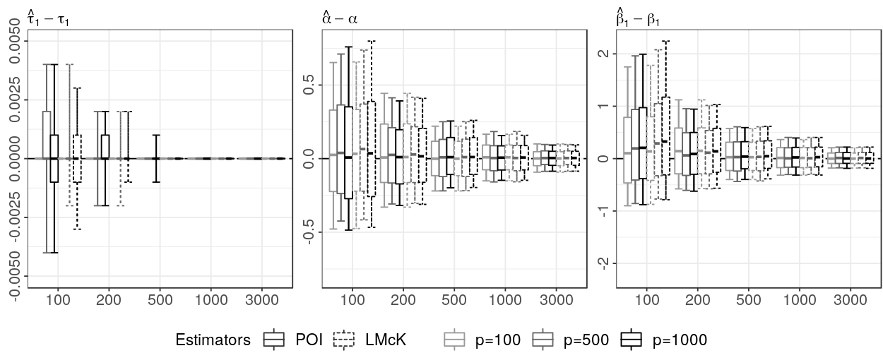 Figure 4
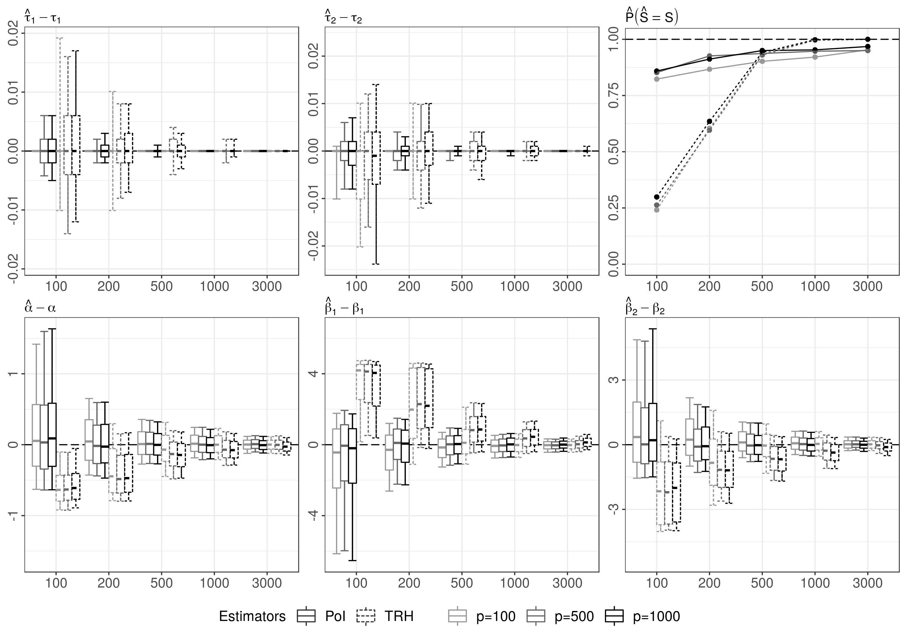 Figure 5
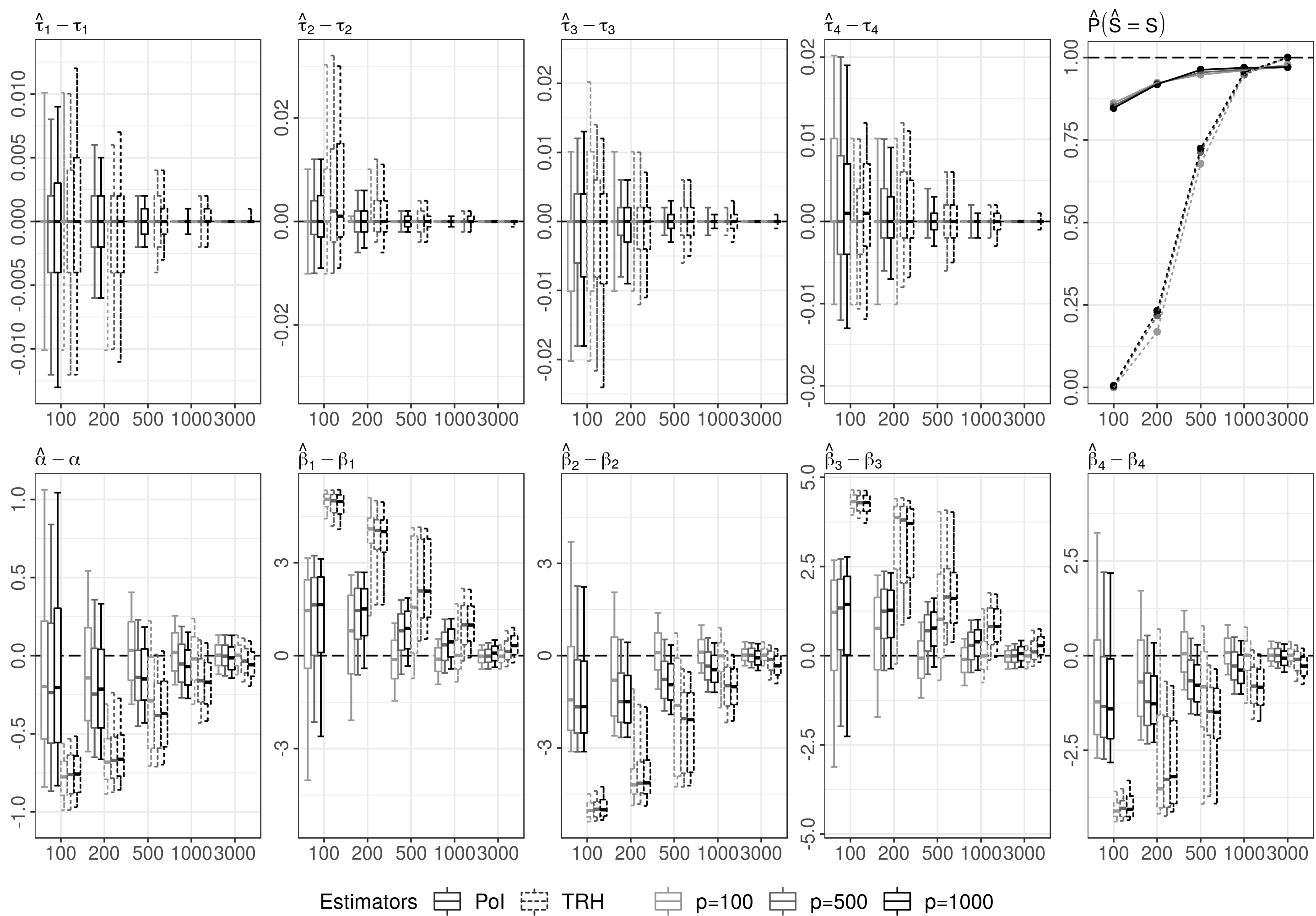 Figure 6
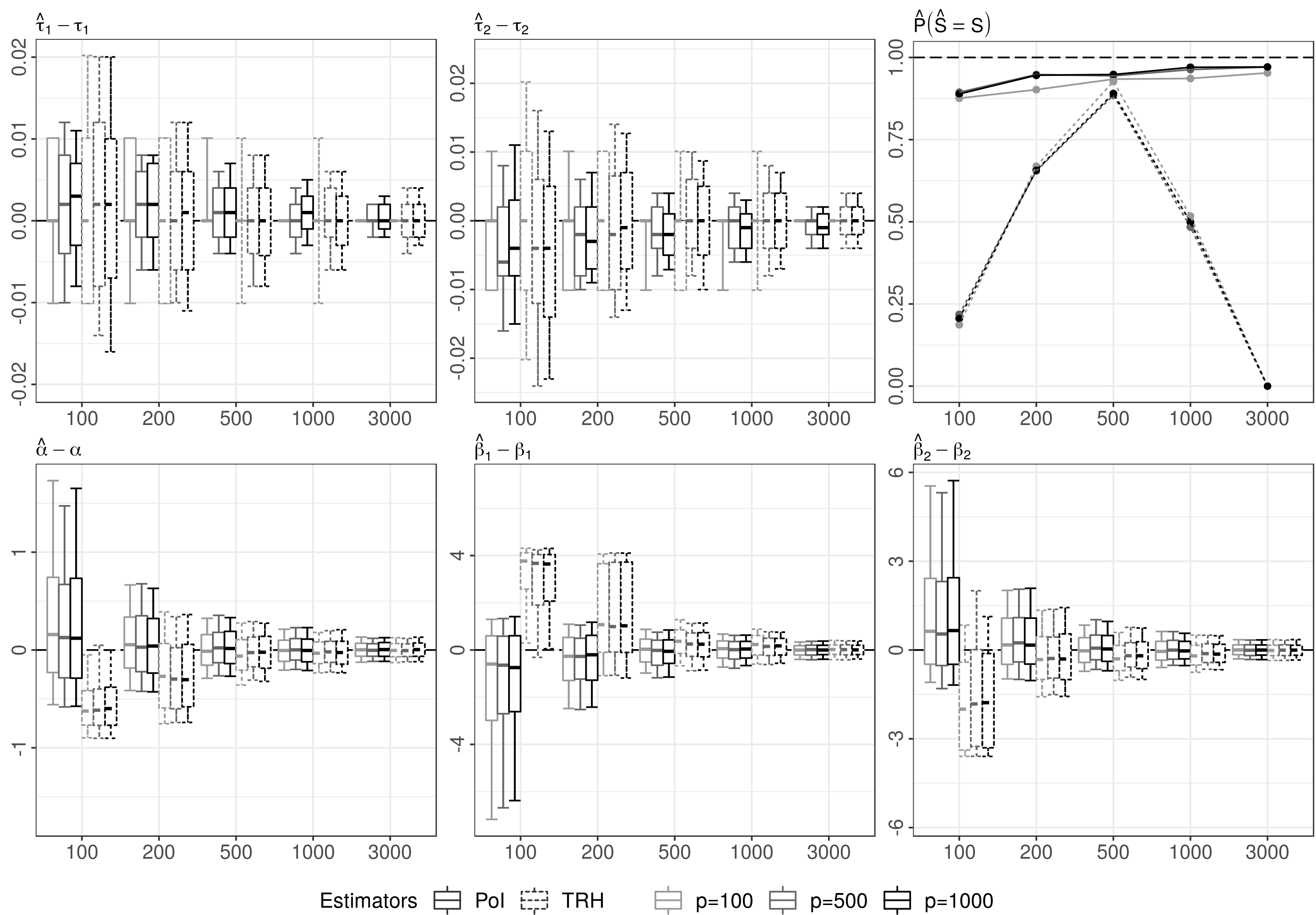 Figure 7
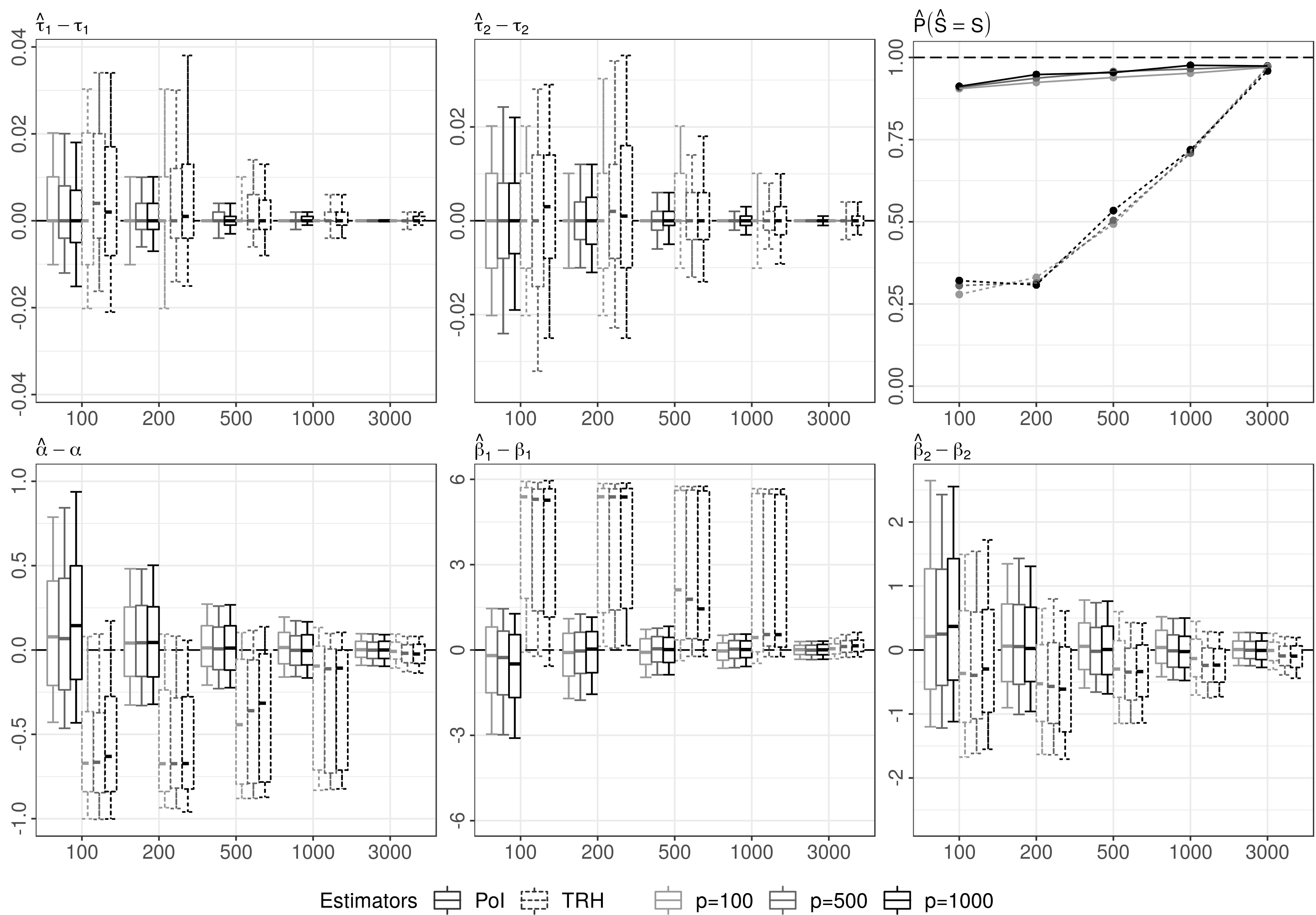 Figure 8
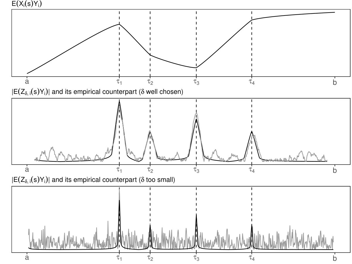 Figure 2
 Figure 10
| MASE | ||||
|---|---|---|---|---|
| DGP | TRH | MPDP | ||
| 2 | 100 | 100 | 0.098 | 0.100 |
| 2 | 100 | 200 | 0.061 | 0.089 |
| 2 | 100 | 500 | 0.017 | |
| 2 | 500 | 100 | 0.097 | 0.098 |
| 2 | 500 | 200 | 0.064 | 0.092 |
| 2 | 500 | 500 | 0.023 | |
| 2 | 1000 | 100 | 0.094 | |
| 2 | 1000 | 200 | 0.060 | |
| 2 | 1000 | 500 | 0.022 | |
| 3 | 100 | 100 | 0.155 | 0.175 |
| 3 | 100 | 200 | 0.105 | 0.156 |
| 3 | 100 | 500 | 0.058 | |
| 3 | 500 | 100 | 0.150 | 0.173 |
| 3 | 500 | 200 | 0.102 | 0.161 |
| 3 | 500 | 500 | 0.060 | |
| 3 | 1000 | 100 | 0.149 | |
| 3 | 1000 | 200 | 0.100 | |
| 3 | 1000 | 500 | 0.059 | |
| AvgMSE | ||||
|---|---|---|---|---|
| DGP | TRH | MPDP | ||
| 2 | 100 | 100 | 0.0002 | 0.0063 |
| 2 | 100 | 200 | 0.0001 | 0.0023 |
| 2 | 100 | 500 | 0.0000 | |
| 2 | 500 | 100 | 0.0002 | 0.0084 |
| 2 | 500 | 200 | 0.0001 | 0.0013 |
| 2 | 500 | 500 | 0.0000 | |
| 2 | 1000 | 100 | 0.0002 | |
| 2 | 1000 | 200 | 0.0001 | |
| 2 | 1000 | 500 | 0.0000 | |
| 3 | 100 | 100 | 0.0002 | 0.0186 |
| 3 | 100 | 200 | 0.0001 | 0.0036 |
| 3 | 100 | 500 | 0.0000 | |
| 3 | 500 | 100 | 0.0002 | 0.0218 |
| 3 | 500 | 200 | 0.0001 | 0.0035 |
| 3 | 500 | 500 | 0.0000 | |
| 3 | 1000 | 100 | 0.0002 | |
| 3 | 1000 | 200 | 0.0001 | |
| 3 | 1000 | 500 | 0.0000 | |
Peer Reviews
No public reviews on file for this paper yet. If you reviewed it on a platform where reviews are public (OpenReview, ICLR, NeurIPS, ICML), you can paste yours below so the community can read it here.
Videos
No videos yet. Explain this paper in a talk, walkthrough, or lecture? Add one.
\newcites
appendixReferences
Super-Consistent Estimation of Points of Impact in Nonparametric Regression with Functional Predictors
Dominik Poß, Dominik Liebl, Alois Kneip††footnotemark: , Hedwig Eisenbarth, Tor D. Wager, Institute of Finance and Statistics, University of Bonn, Bonn, GermanyInstitute of Finance and Statistics and Hausdorff Center for Mathematics, University of Bonn, Bonn, GermanySchool of Psychology, Victoria University of Wellington, Wellington, New ZealandPresidential Cluster in Neuroscience and Department of Psychological and Brain Sciences, Dartmouth College, Hanover, New Hampshire, USA
and Lisa Feldman Barrett Department of Psychology, Northeastern University and Department of Psychiatry, Massachusetts General Hospital/Harvard Medical School, Boston, Massachusetts, USA; and Athinoula A. Martinos Center for Biomedical Imaging, Massachusetts General Hospital, Charlestown, Massachusetts, USA
Abstract
Predicting scalar outcomes using functional predictors is a classic problem in functional data analysis. In many applications, however, only specific locations or time-points of the functional predictors have an impact on the outcome. Such “points of impact” are typically unknown and have to be estimated in addition to estimating the usual model components. We show that our points of impact estimator enjoys a super-consistent convergence rate and does not require knowledge or pre-estimates of the unknown model components. This remarkable result facilitates the subsequent estimation of the remaining model components as shown in the theoretical part, where we consider the case of nonparametric models and the practically relevant case of generalized linear models. The finite sample properties of our estimators are assessed by means of a simulation study. Our methodology is motivated by data from a psychological experiment in which the participants were asked to continuously rate their emotional state while watching an affective video eliciting a varying intensity of emotional reactions.
Keywords: functional data analysis; variable selection; nonparametric regression; quasi-maximum likelihood; emotional stimuli; online video rating
1 Introduction
Identifying important time points in time continuous trajectories is a difficult but highly relevant problem. For instance, current psychological research on emotional experiences often includes time continuous stimuli such as videos to induce emotional states, say , with , where denotes the start of the video and the end (see Figure 1). The evaluation of such stimuli is based on asking participants whether the video made them feel negative, say , or positive, say . In this paper we consider a novel dataset where participants were asked to continuously report their emotional states while watching an affective documentary video on the persecution of African albinos. After watching the video, the participants were asked to rate their final overall feeling. Psychologists are interested in understanding how such concluding overall ratings relate to the fluctuations of the emotional states while watching the video, as this has implications for the way emotional states are assessed in research using such material. Due to a lack of appropriate statistical methods, existing approaches use heuristics such as the “peak-and-end rule” in order to link the overall ratings with the continuous emotional stimuli (see Section 5). Such heuristic approaches, however, can produce results that do not accurately capture the summary rating and can be easily over-interpreted, as there is no unbiased formal inference about which time points contribute to the summary rating. By contrast, our new methodology allows us to identify the crucial affective video scenes – the basic prerequisite to understanding the emergence of emotional states in this kind of experiment.
The identification of “influential” stimuli occurring in a video corresponds to identify corresponding time points . We aim to estimate such time points within the nonparametric model
[TABLE]
where and their number are unknown and need to be estimated. The values are called points of impact and provide specific locations at which the functional predictor influences the scalar outcome . In our real data application in Section 5, is a binary variable and the functional predictor is evaluated at two estimated points of impact and ; see Figure 5.
Our method builds upon the work of Kneip et al. (2016), however, we consider the much more challenging case of estimating points of impact within a fully nonparametric function . A remarkable feature of our method is that identification and estimation of the points of impact neither require knowledge about the nonparametric function nor an estimate of . The estimation of the points of impact is thus robust to model misspecifications and free of additional contaminating estimation errors. This result goes far beyond the special case of a functional linear model as considered by Kneip et al. (2016).
To the best of our knowledge, the problem of estimating in (1) is, so far, only considered by Ferraty et al. (2010), who propose to estimate nonparametrically for any combination of point of impact candidates and to select the best model using cross-validation. This brute force method, however, becomes problematic in practice for and large . Furthermore, the nonparametric estimation of implies that the points of impact can be estimated at most with the non-parametric rate , where denotes the sample size. Here the speed of convergence decreases dramatically for dimensions . By contrast, we can estimate the points of impact with a super-consistent convergence rate, that is, faster than the parametric rate , and our estimation algorithm is applicable in practice for any fixed and large .
The super-consistency result for our points of impact estimators is very beneficial for subsequent estimation problems and allows us to estimate the unknown function as if the points of impact were known. We demonstrate this for a nonparametric model as well as for the practically relevant case of generalized linear models with linear predictors, that is, with assumed known parametric link function .
So far, the purely nonparametric framework is only considered by Ferraty et al. (2010). The case of a known and linear predictor function had already been considered by previous studies; however, none of these studies provides a super-consistent estimation of points of impact independent of the model . The term “impact point” was coined by Lindquist and McKeague (2009) and McKeague and Sen (2010). Lindquist and McKeague (2009) consider a logistic regression framework and McKeague and Sen (2010) consider a linear regression framework. A point of impact model, where is assumed known, has also been studied in survival analysis for the Cox regression model (Zhang, 2012). Kneip et al. (2016) allow for an unknown number of points of impact augmenting the functional linear regression model. Liebl et al. (2020) propose an improved estimation algorithm for the latter work. Aneiros and Vieu (2014) consider a linear regression framework with multiple points of impact postulating the existence of some consistent estimation procedure. Berrendero et al. (2019) consider a linear regression framework and propose a reproducing kernel Hilbert space approach. Selecting sparse features from functional data is also useful for clustering. For instance, Floriello and Vitelli (2017) propose a method for sparse clustering of functional data. In a slightly different context, Park et al. (2016) focus on selecting predictive subdomains of the functional data. Related to this paper is also the work of Lindquist (2012) and Sobel and Lindquist (2014). Lindquist (2012) extends structural equation models to the functional data analysis setting and uses his methodology to select significantly impacting time-intervals in functional magnetic resonance imaging (fMRI) data. Sobel and Lindquist (2014) propose a mixed effects model which facilitates selecting significant impact regions in fMRI data by controlling for systematic measurement errors.
The rest of this work is structured as follows. Section 2 considers the estimation of the points of impact and their number independent of the model . Subsequent estimation of the function is discussed in Section 3. The simulation study and the real data application are in Sections 4 and 5. All proofs and additional simulation results can be found in the appendixes of the supplementary paper supporting this article (Poß et al., 2020). The R-package fdapoi and the R-scripts for reproducing our main empirical results are also provided as part of the online supplementary material (Poß et al., 2020).
2 Estimating points of impact
In the following we present our theoretical framework (Section 2.1), the estimation algorithm (Section 2.2) and our asymptotic results (Section 2.3). The section concludes with a discussion of possibilities to generalize our theoretical results (Section 2.4).
2.1 Theoretical framework
In this section we present our theoretical framework for estimating the points of impact without knowing or (pre-)estimating the possibly nonparametric model function . The identification of points of impact constitutes a particular variable selection problem. Since we consider the case where the functional predictor is observed over a densely discretized grid, one might be tempted to apply multivariate variable selection methods like Lasso or related procedures. Note, however, that the high correlation of the predictor at neighboring discretization points violates the basic requirements of these multivariate variable selection procedures.
Suppose we are given an i.i.d. sample of data , , where is a stochastic process with , is a compact subset of and is a real valued random variable. It is assumed that the relationship between and the functional predictor can be modeled as
[TABLE]
where denotes the statistical error term with for all . The number and the points of impact are unknown and have to be estimated from the data – without knowing the true model function . The points of impact indicate the locations at which the functional values have a specific influence on . Without loss of generality, we consider centered random functions with for all .
Surprisingly, the unknown function has to fulfill only some very mild regularity conditions and does not have to be estimated in order to estimate the points of impact (see Theorem 2.1). Estimating points of impact, however, necessarily depends on the structure of . Motivated by our application we consider stochastic processes with rough sample paths such as (fractional) Brownian motion, Ornstein-Uhlenbeck processes, Poisson processes, etc. These processes also have important applications in fields such as finance, chemometrics, econometrics, and the analysis of gene expression data (Lee and Ready, 1991; Levina et al., 2007; Dagsvik and Strøm, 2006; Rohlfs et al., 2013). Common to these processes are covariance functions which are two times continuously differentiable for all points , but not two times differentiable at the diagonal . The following assumption on the covariance function of describes a very large class of such stochastic processes and allows us to derive precise theoretical results:
Assumption 2.1**.**
For some open subset with , there exists a twice continuously differentiable function as well as some such that for all
[TABLE]
Moreover, , where .
The parameter quantifies the degree of smoothness of the covariance function at the diagonal. While a twice continuously differentiable covariance function will satisfy (3) with , small values indicate a process with non-smooth sample paths.
Assumption 2.1 covers several important classes of stochastic processes. Recall, for instance, that the class of self-similar (not necessarily centered) processes has the property that for any constant and some exponent . It is then well known that the covariance function of any such process with stationary increments and satisfies
[TABLE]
for some constant ; see Theorem 1.2 in Embrechts and Maejima (2000). If such a process respects Assumption 2.1 with and . A prominent example of a self-similar process is the fractional Brownian motion.
Another class of processes is given when is a second order process with stationary and independent increments. In this case it is easy to show that for some constant . The Assumption 2.1 then holds with and . The latter conditions on are, for instance, satisfied by second order Lévy processes which include important processes such as Poisson processes, compound Poisson processes, or jump-diffusion processes.
A third important class of processes satisfying Assumption 2.1 are those with a Matérn covariance function. For this class of processes the covariance function depends only on the distance between and through
[TABLE]
where is the modified Bessel function of the second kind, and , and are non-negative parameters of the covariance. It is known that this covariance function is times differentiable if and only if (cf. Stein, 1999, Ch. 2.7, p. 32). Assumption 2.1 is then satisfied for . For the special case where one may derive the long term covariance function of an Ornstein-Uhlenbeck process which is given as , for some parameter and . Assumption 2.1 is then covered with and .
The remarkable result that identification and estimation of the points of impact requires neither knowledge about the possibly nonparametric function nor an estimate of is based on the following theorem.
Theorem 2.1**.**
Let be a Gaussian process. For any function such that for all the partial derivative is continuous almost everywhere and , we define \vartheta_{r}=\operatorname{\mathbb{E}}\big{(}\frac{\partial}{\partial x_{r}}g(X_{i}(\tau_{1}),\dots,X_{i}(\tau_{S}))\big{)}. Then the equation \operatorname{\mathbb{E}}\big{(}X_{i}(s)Y_{i}\big{)}=\sum_{r=1}^{S}\vartheta_{r}\sigma(s,\tau_{r}) holds for all .
Theorem 2.1 allows to decompose the cross-covariance into coefficients , which depend on the unknown function , and the covariance function , which only depends on . Our estimation strategy for the points of impact works for unknown with . The latter imposes only mild regularity assumptions on and is fulfilled, for instance, by any nonparametric single-index model, with , where . Of course, the class of possible functions defined by Theorem 2.1 also contains much more complex cases than single-index models.
The intention of our estimator for the points of impact is to exploit the covariance structure of processes described by Assumption 2.1. Covariance functions satisfying Assumption 2.1 are obviously not two times differentiable at the diagonal , but are two times differentiable for . Using Theorem 2.1 in conjunction with Assumption 2.1 allows us to uniquely identify the locations of the points of impact from the cross-covariance . Let us make this more precise by defining
[TABLE]
Since is not two times differentiable at , the cross-covariance will not be two times differentiable at , for all , resulting in kink-like features at as depicted in the upper plot of Figure 2.
A natural strategy for estimating is to detect these kinks by considering the following modified central difference approximation of the second derivative of at a point for some :
[TABLE]
By defining the auxiliary process
[TABLE]
we have the following equivalent moment expression for (4):
[TABLE]
At , expression (5) will decline more slowly to zero as than for , . For suitable values of , the points of impact can then be estimated using the local extrema of the empirical counterpart of (see middle panel of Figure 2).
More precisely, Theorem 2.1 together with Proposition C.1 and Lemma C.4 in Appendix C of the supplementary paper Poß et al. (2020) imply that as
[TABLE]
where and are as defined in Assumption 2.1.
Of course, is not known and we have to rely on as its estimate. Under our setting we will have that the variance which implies
[TABLE]
Consequently, the identification of points of impact requires a sensible choice of . For too small -values (e.g., ) the estimation noise will overlay the signal; this situation is depicted in the bottom plot of Figure 2. For too large -values, however, it will not be possible to distinguish between neighboring points of impact.
Remark: Even if the covariance function does not satisfy Assumption 2.1, the points of impact may still be estimated using the local extrema of . Suppose, for instance, there exists a times differentiable function such that , where decays fast enough, as increases, such that is essentially uncorrelated with for . If , for , and is large enough, then all points of impact might be identified as local extrema of .
2.2 Estimation algorithm
In the following we consider the case where each has been observed over equidistant points , , where may be much larger than . Estimators for the points of impact are determined by sufficiently large local maxima of .
Algorithm 2.1**.**
(Estimating points of impact)**
- 1.
Calculate* * 2. 2.
Choose* such that there exists some with and .* 3. 3.
Calculate* , for all , where * 4. 4.
Repeat:**
- Initiate* the repetition by setting .*
- Estimate* the **th point of impact candidate as
- Update* by eliminating all points in in an interval of size around .*
Update* Set .*
- End* repetition if .*
The procedure will result in estimates , where denotes the maximum number of possible repetitions. The estimator of is
[TABLE]
An asymptotically valid choice of the threshold is presented in Theorem 2.2 and a practical implementation of is discussed below of Theorem 2.2.
Remark: * This estimation algorithm is made for the case of densely observed functional data. In practice this means functional data that are sampled at a high frequency such as in our real data example (Section 5). Unfortunately, we do not see a simple way to generalize our method to the case of irregularly or sparsely sampled functional data. Such a generalization would require a very different approach based on nonparametric smoothing procedures.*
2.3 Asymptotic results
In this section, we consider asymptotics as with for some constant . We introduce the following assumption:
Assumption 2.2**.**
- a)
* are i.i.d. random functions distributed according to . The process is Gaussian with covariance function .*
- b)
*There exists a such that for each we have *
.
The moment condition in b) is obviously fulfilled for bounded . For instance, in the functional logistic regression we have that for all . Condition b) also holds for any centered sub-Gaussian , where a centering of can always be achieved by substituting for in Model (2). If satisfies condition a), then condition b) in particular holds if the errors are sub-Gaussian and is differentiable with bounded partial derivatives.
The following result shows consistency of our estimators for the points of impact and the estimator :
Theorem 2.2**.**
Under Assumptions 2.1, 2.2, and the assumptions of Theorem 2.1, let as such that and . We then obtain that
[TABLE]
Moreover, there exists a constant such that when Algorithm 2.1 is applied with threshold
[TABLE]
[TABLE]
Note that the rates of convergence in (6) are super-consistent, since . For instance, for Ornstein-Uhlenbeck processs or Brownian motions we have , such that .
In principle, arbitrarily fast rates of convergence can be achieved for -values close to zero, because small -values correspond to rough processes, . Roughness means that the process has strong local variations also within small intervals , , which facilitates differentiating a point of impact , , from the neighboring points . By contrast, for smooth processes (large -values) all values of with will be almost identical which makes it hard to identify the correct point of impact .
A practical and asymptotically valid threshold specification which performed well in our simulation studies is given by \lambda=A((\operatorname{\mathbb{E}}(Y_{i}^{4}))^{1/2}\log\big{(}(b-a)/\delta\big{)}/n)^{1/2}, where is estimated by and . This value is motivated by an argument using the central limit theorem in the derivations of the threshold for Theorem 2.2. See the remark after the proof of Lemma C.3 in Appendix C for additional information.
The super-consistency result in Theorem 2.2 is very general and does not require knowledge of or a pre-estimate of ; only a set of mild and verifiably assumptions on is postulated. Therefore, we expect that the theorem will be found useful for deriving inferential results for a broad variety of different models . In the following we demonstrate the usefulness of Theorem 2.2 for deriving inferential results for nonparametric models and parametric generalized linear models. Note that the related Corollary 1 in Ferraty et al. (2010) requires the simultaneous estimation of the nonparametric model function and the points of impact. This approach results in substantially slower nonparametric convergence rates and limits the applicability of their result considerably.
2.4 Generalizations
The above theoretical assumptions provide a tractable setup that will be used also in the remaining parts of the paper. In this subsection, however, we show that the Gaussian assumption of Theorem 2.1 and Theorem 2.2 can be relaxed and that our approach for identifying and estimating the points of impact may also work for a large class of non-Gaussian processes (Section 2.4.1). Moreover, we outline how our estimation procedure can be adapted to a more general version of the covariance Assumption 2.1 (Section 2.4.2).
2.4.1 Non-Gaussian processes
To generalize Theorem 2.1 one can build upon the framework of elliptical processes which includes the case of non-Gaussian, heavy-tailed distributions. That is, one can consider processes that depend on some latent random variable such that the conditional distribution of given is Gaussian. However, the (unconditional) distribution of then additionally depends on the distribution of and may be far from Gaussian.
Our conditions A and B in Appendix B.2 define a general framework for such non-Gaussian processes and Proposition B.1 in Appendix B.2 generalizes Theorem 2.1 for this general framework. Here in this subsection, however, we focus on the arguably most important special case of our general framework – namely, the case of elliptically distributed processes. Elliptical distributions include the special case of a Gaussian distribution as considered in Theorem 2.1, but also many important non-Gaussian distributions such as the t-distribution, the Laplace distribution, and the logistic distribution (see, for instance, Boente et al., 2014).
Let be a (centered) elliptical process, that is, let , , where is a strictly positive real-valued random variable, is a zero mean Gaussian process with covariance function , and where and are independent of each other. Moreover, let the error term in (2) be independent of and and let . Then the elliptically distributed random function fulfills our conditions A and B in Appendix B.2 and it follows by Proposition B.1 in Appendix B.2 that
[TABLE]
where \vartheta_{r}(V_{i})=\operatorname{\mathbb{E}}\big{(}\frac{\partial}{\partial x_{r}}g(X_{i}(\tau_{1}),\dots,X_{i}(\tau_{S}))\big{|}V_{i}\big{)} and is the covariance function of the elliptically distributed process . As in the case of Theorem 2.1, the above result allows us to decompose the cross-covariance into a scaling coefficient which depends on the unknown function (via ) and the covariance function which only depends on . This result holds for elliptically distributed and requires only mild regularity assumptions on which are essentially equivalent to those imposed by Theorem 2.1; see conditions A and B in Appendix B.2.
As in the preceding section, the identification of the points of impact relies only on the structural covariance Assumption 2.1 which holds for rough – Gaussian or non-Gaussian – processes . Since , the requirements of Assumption 2.1 may directly be applied to the covariance function of the Gaussian process component of the elliptical process . If satisfies Assumption 2.1 for some , then Proposition B.1 in Appendix B.2 leads to
[TABLE]
as with , where , .
Theorem 2.2 can also be generalized to the case that is elliptically distributed. Note that then , where , for , and . Therefore, estimating points of impact from data is equivalent to estimating points of impact from data . Thus, Theorem 2.2 remains valid if all conditions on and in Theorem 2.2 now apply to and .
Our more general framework of conditions A and B in Appendix B.2 includes even more complex cases than the above discussed elliptical processes. For instance, one may consider processes , where is jointly independent of and where and are almost surely twice continuously differentiable functions on (see Appendix B.2 in the supplementary paper Poß et al. (2020) for more details).
2.4.2 Generalizing covariance Assumption 2.1
Assumption 2.1 holds for non-smooth/rough processes with covariance function , where the requirement excludes all smooth, twice continuously differentiable processes, , with .
However, the degree of roughness of the processes, , is actually not a necessary requirement for identifying and estimating points of impact. The crucial property is that the covariance function of is less smooth at the diagonal than for . For instance, let be times continuously differentiable at all off-diagonal points, , but not times differentiable at the diagonal points, . This scenario corresponds to a generalization of Assumption 2.1 with which now excludes only all four times continuously differentiable processes, , with . In this case, one may look at the modified th central difference approximation of the th derivative of and replace by
[TABLE]
Theoretical results may then be derived under a generalized version of Assumption 2.1 demanding that there exists a times differentiable function such that (3) holds for any .
Equivalent generalizations can, for instance, be made for any , which would involve then a modified th order central difference processes . This way, Assumption 2.1 can be generalized to the requirement which also then includes smooth processes, . Deriving the estimation theory under this setup would then lead to even more accurate points of impact estimators with an even faster super-consistent convergence rate. However, taking higher order differences in practice usually involves numerical instabilities.
3 Subsequent estimation of
Given estimates of the points of impact and their number , one is typically interested in the subsequent estimation and inference regarding the remaining model components. The following section considers the case of a nonparametric model . Section 3.2 considers the case of a generalized linear model, which is of particular practical relevance.
In the following we assume the existence of some consistent estimation procedure for the points of impact satisfying and , where we use matched labels in the sense that . These requirements are fulfilled by our estimation procedure described in Section 2.2, but may also be fulfilled for alternative procedures.
3.1 Nonparametric estimation
Estimating the nonparametric function in (2) is a non-standard estimation problem, since the unknown points of impact of the predictor variables must be replaced by their estimates . That is, for given estimates we may estimate the unknown regression function by the following Nadaraya-Watson type estimator
[TABLE]
where denotes a standard nonnegative symmetric bounded second-order kernel function with , and where denote the bandwidth parameters.
For the following result we make use of our super-consistency result in Theorem 2.2. Note, however, that the rates of consistency for the point of impact estimators of Theorem 2.2 cannot be used directly to quantity the errors , , since under Assumption 2.1 we cannot make use of Taylor-expansions of . Therefore, the following result is non-standard because of the additional error component \widehat{g}_{\widehat{\tau}}(x_{1},\dots,x_{S})-\widehat{g}_{\tau}(x_{1},\dots,x_{S})=O_{p}\big{(}\sum_{r=1}^{S}1/(n^{\min\{1,1/\kappa\}}(h_{1}\cdots h_{S})h_{r}^{2})\big{)} contained in (9), where is defined as in (8), but using the true predictor variables .
Theorem 3.1**.**
Let , , and let Assumptions 2.1 and 2.2 and the assumptions of Theorem 2.2 hold. Moreover, let the kernel function be a second-order kernel (i.e., a density function that is symmetric around zero) with continuous second-order partial derivatives and let the regression function have continuous second-order partial derivatives. We then have for any points in the interior of the support of that
[TABLE]
for , and with , for each .
If each bandwidth has the same order of magnitude and , the well-known optimal bandwidth choice , , can be used to simplify Theorem 3.1 as following.
Corollary 3.1**.**
Under the assumptions of Theorem 3.1, let and for all . Then
[TABLE]
That is, under the conditions of Corollary 3.1, we have the same optimal rates of convergence as in the case where the points of impact were known.
3.2 Parametric estimation
In this section it is assumed that the relationship between and the functional predictor can be modeled using the framework of generalized linear models with known parametric function ,
[TABLE]
in which the i.i.d. error term respects for all and where with strictly positive variance function defined over the range of . For simplicity the function is assumed to be a known, strictly monotone and smooth function with bounded first and second order derivatives and hence invertible (see, for instance, Müller and Stadtmüller, 2005, for similar assumptions). The constant allows us to consider centered random functions with for all . Note that we do not assume that the conditional distribution of belongs to the exponential family of distributions. Denoting the linear predictor
[TABLE]
allows us to write as well as . Hence, this setup of model (10) belongs to the broad class of quasi-likelihood models which can be seen as a generalization of a generalized linear model framework (cf. McCullagh and Nelder, 1989, Ch. 9).
Identifiability of the model parameters in (10) is not obvious due to the functional predictor , which, in principle, allows for infinitely many alternative model candidates. The following Theorem 3.2 shows that any possible kind of model-misspecification in , , , , or , will lead to a different model in the mean squared error sense implying the identifiability of model (10).
Theorem 3.2**.**
Let be invertible and assume that satisfies Assumptions 2.1 and 2.2. Then for all , all , and all with , , we obtain
[TABLE]
whenever , or , or .
Note that the proof of Theorem 3.2 does only require the existence of second moments and, therefore, may be generalized also to the case of non-Gaussian processes .
Estimation of is performed by quasi-maximum likelihood. Define and denote the th, , element of the latter vector as . For let , , be the matrix with entries , and let be a diagonal matrix with elements . Furthermore, denote the corresponding objects evaluated at the true points of impact by , , , , , and ; this notational convention applies also to the below defined objects.
Our estimator for is defined as the solution of the score equations , where
[TABLE]
Note that these are non-classic score equations evaluated at the estimates instead of .
In the following, it will be convenient to define
[TABLE]
By definition it holds that with . Let and be generic copies of and of the th component of , respectively. This allows us to write with , where we point out that is for all a symmetric and strictly positive definite matrix with inverse . Indeed, suppose were not strictly positive definite, we would then derive the contradiction for nonzero constants . A similar argument can be used to show that is strictly positive definite, where .
The following additional set of assumptions are used to derive more precise theoretical statements:
Assumption 3.1**.**
- a)
There exists a constant , such that , for all and for some even with and some .
- b)
The function is monotone, invertible with two bounded derivatives , , for some constant .
- c)
* is a bounded function with two bounded derivatives.*
Condition a) states that some higher moments of exist. While the condition on and being even simplifies the proofs, the condition is a more crucial one and is used in the proof of Proposition D.2 in the supplementary Appendix D.2. Conditions a) to c) hold, for example, in the important case of a functional logistic regression with points of impact, where is the standard logistic function. Condition c) is satisfied, for instance, in the special case of generalized linear models with natural link functions. For the latter case, we have such that .
Theorem 3.3**.**
Let , and let be a Gaussian process satisfying Assumption 2.1. Under Assumption 3.1 we then obtain
[TABLE]
That is, our estimator based on enjoys the same asymptotic efficiency properties as if the true points of impact were known. In fact, it achieves the same asymptotic efficiency properties as under classic multivariate setups (cf. McCullagh, 1983). In practice one might replace with its consistent estimator in order to derive approximate results. This is a direct consequence of Equations (129) and (155) in the supplementary Appendix D.2.
3.2.1 Parametric estimation: Practical implementation
An implementation of our parametric estimation procedure comprises, first, the estimation of the points of impact and, second, the estimation of the parameters and . Estimating the points of impact relies on the choice of and a choice of the threshold parameter (see Section 2.2). Asymptotic specifications are given in Theorem 2.2; however, these determine the tuning parameters and only up to constants and are generally of a limited use in practice. In the following we propose an alternative fully data-driven model selection approach.
For a given , our estimation procedure leads to a set of potential point of impact candidates (see Section 2.2). Selecting final point of impact estimates from this set of candidates corresponds to a classic variable selection problem. In the case where the distribution of belongs to the exponential family (as in the logistic regression) one may perform a best subset selection optimizing a standard model selection criterion such as the Bayesian Information Criterion (BIC),
[TABLE]
Here, is the log-likelihood of the model with intercept and predictor variables , where denotes the number of predictors. Minimizing over leads to the final model choice.
In the more general case of quasi-likelihood models (cf. McCullagh and Nelder, 1989, Ch. 9) where only the first two moments and are known, one may replace the deviance by the expression for the quasi-deviance , where is the linear predictor with intercept and predictor variables .
In order to calculate , we need the estimates solving the estimation equations . In practice these equations are solved iteratively, for instance, by the usual Newton-Raphson method with Fisher-type scoring. That is, for an arbitrary initial value sufficiently close to one generates a sequence of estimates , with ,
[TABLE]
Iteration is executed until convergence and the final step of the procedure yields the estimate . Here, and replace and in the usual Fisher scoring algorithm, since the unknown , , are replaced by their estimates . The latter is justified asymptotically by our results in Corollary D.1 and Proposition D.3 in Appendix D.2.
4 Simulation
We investigate the finite sample performance of our estimators using Monte Carlo simulations. After simulating a trajectory over equidistant grid points , , on , linear predictors of the form are constructed for some predetermined model parameters , , , and , where a point of impact is implemented as the smallest observed grid point closest to . The response is derived as a realization of a Bernoulli random variable with success probability , resulting in a logistic regression framework with points of impact. The simulation study is implemented in R (R Core Team, 2020), where we use the R-package glmulti (Calcagno, 2013) in order to implement the fully data-driven BIC-based best subset selection estimation procedure described in Section 3.2.1. The threshold estimator from Section 2.2 requires appropriate choices of and . Theorem 2.2 suggests that a suitable choice of is given by for some constant . Our simulation results are based on ; similar qualitative results were derived for a broader range of values . For the threshold we use , where and , as motivated below of Theorem 2.2.
In what follows, we denote the BIC-based selection (see Section 3.2.1) of points of impact by POI and the threshold-based selection (Algorithm 2.1) by TRH. Estimated points of impact candidates are related to the true impact points by the following matching rule: In a first step the interval is partitioned into subintervals of the form , where , and for . The candidate in interval with the closest distance to is then taken as the estimate of .
The simulation results for our parametric estimation procedure (Section 3.2) are based on Monte Carlo iterations for each constellation of and . The results for our nonparametric estimation procedure (Section 3.1), are based on the same general setup, but consider the reduced set of sample sizes . Estimation errors for the parametric estimation procedure are illustrated by boxplots with error bars representing the and quantiles. The estimation errors for the nonparametric estimation procedure are quantified by the Mean Average Squared Error, \operatorname{MASE}=1000^{-1}\sum_{r=1}^{1000}n^{-1}\sum_{i=1}^{n}\big{(}g(\eta_{i})-\widehat{g}^{r}_{\widehat{\tau}}(X^{r}_{i}(\widehat{\tau}^{r}_{1}),\dots,X^{r}_{i}(\widehat{\tau}^{r}_{\hat{S}}))\big{)}^{2}, where the superscript denotes the th simulation run.
Five data generating processes (DGP) are considered (see Table 1) using the following three processes covering a broad range of situations:
OUP
Ornstein-Uhlenbeck Process. A Gaussian process with covariance function . We choose and .
GCM
Gaussian Covariance Model. A Gaussian process with covariance function . We choose .
EBM
Exponential Brownian Motion. A non Gaussian process with covariance function . It is defined by , where is a Brownian motion.
DGP 1-3 are increasingly complex, but satisfy our theoretical assumptions. The general setups of DGP 4 and DGP 5 are equivalent to DGP 2, but the processes (GCM and EBM) violate our theoretical assumptions. The covariance function in DGP 4 is infinitely many times differentiable, even at the diagonal where , contradicting Assumption 2.1, but fitting the remark underneath this Assumption. The process in DGP 4 contradicts the Gaussian Assumption 2.2.
4.1 Evaluation of the parametric estimation procedure
DGP 1 allows us to compare our data-driven BIC-based estimation procedure from Section 3.2.1 (denoted as POI) with the estimation procedure of Lindquist and McKeague (2009) (denoted as LMcK). Lindquist and McKeague (2009) consider situations where is known and propose estimating the unknown parameters and by simultaneously maximizing the likelihood over , and the grid points . Our estimation procedure does not require knowledge about , but profits from a situation where is known. Therefore, for reasons of comparability, we restrict the BIC-based model selection process to allow only for models containing one point of impact candidate. The simulation results are depicted in Figure 3 and are virtually identical for both methods and show a satisfying behavior of the estimates. It should be noted, however, that our estimator is computationally advantageous as it greatly thins out the number of possible point of impact candidates by allowing only the local maxima of as possible point of impact candidates. Our threshold-based estimation procedure leads to similar qualitative results. We omit these results, however, in order to allow for a clear display in Figure 3. The performance of our threshold-based procedure is reported in detail for the remaining simulation studies (DGP 2-5).
DGP 2 is more complex than DGP 1 since and considered unknown. Figure 4 compares the estimation errors from using our BIC-based POI estimator with those from our threshold-based estimator (denoted as TRH). For smaller sample sizes , the POI estimator seems to be preferable to the TRH estimator. Although, estimating the locations of the points of impact and is quite accurate for both procedures, the number is estimated correctly more often using the POI estimator (see upper right panel). The more precise estimation of when using the POI estimator results in essentially unbiased estimates of the parameters , , and . By contrast, the less precise estimation of using the TRH estimator leads to clearly visible omitted variable biases in the estimates of the parameters , , and . As the sample size increases, however, the accuracy of estimating improves for the TRH estimator such that both estimators show eventually a similar performance.
DGP 3 with unknown points of impact comprises an even more complex situation than DGP 2. For reasons of space, Figure 7 is referred to Appendix A. It shows that the qualitative results from DGP 2 still hold. For large , the POI and TRH estimators both lead to accurate estimates of the model parameters for all choices of . As already observed in DGP 2, however, the TRH estimator leads to imprecise estimates of for small , which results in omitted variables biases in the estimates of the parameters , , , , and . Because of the increased complexity of DGP 3, these biases are even more pronounced than in DGP 2. The reason for this is partly due to the construction of the TRH estimator, where we set the value of to with . Asymptotically, the choice of has a negligible effect, but may be inappropriate for small , since the estimation procedure eliminates all points within a -neighborhood around a chosen candidate (see Section 2.2). For DGP 3, the choice of results in a too large -neighborhood, such that the estimation procedure also eliminates true point of impact locations for small . By contrast, the POI estimator is able to avoid such adverse eliminations as the BIC criterion is also minimized over .
DGP 4 takes up the general setup of DGP 2, but the functional data are simulated using a Gaussian covariance model (GCM) which is characterized by an infinitely many times differentiable covariance function. This setting contradicts our basic Assumption 2.1, but fits our remark at the end of Section 2.1. From Figure 5 it can be concluded that even under the failure of Assumption 2.1, both estimation procedures are capable of consistently estimating the points of impact and the model parameters. The TRH estimator, however, fails to estimate the number of points of impact even for large , since the -threshold is tailored for situations under Assumption 2.1. Here the TRH estimator is able to estimate the true points of impact, but additionally selects more and more redundant point of impact candidates as becomes large. That is, the TRH estimator becomes more a screening than a selection procedure which can be problematic in practice. By contrast, the POI estimator is able to avoid such redundant selections of point of impact candidates, as the BIC criterion only selects points of impact candidates if they result in a sufficiently large improvement of the model fit.
DGP 5 also takes up the setup of DGP 2; however, the process is simulated as an exponential Brownian Motion (EBM) violating Assumption 2.2, but still satisfying Assumption 2.1. Here we set the asymptotically negligible tuning parameter of the TRH estimator equal to 3. The evolution of the estimation errors can be seen in Figure 8 in Appendix A. The results are comparable with our previous simulations in DGP 2 and DGP 3, indicating that the estimation procedure is robust to at least some violations of Assumption 2.2.
4.2 Evaluation of the nonparametric estimation procedure
Table 2 contains the simulation results for our nonparametric estimation procedure described in Section 3.1. We focus on the more challenging data generating processes, DGP2-5, with at least two points of impact and compare our nonparametric method with the Most-Predictive Design Points (MPDP) method of Ferraty et al. (2010). To the best of our knowledge, the MPDP method is the only comparable method in the literature. We tried hard to carry out the full simulation study for the MPDP method; however, Ferraty et al. (2010) use a brute force minimization approach based on cross-validation considering grid point combinations, which makes their method computationally extremely expensive.111Due to the high computational costs, the simulation study in Ferraty et al. (2010) is based on only 50 Monte Carlo replications. In a readme-file, provided at Frederic Ferraty’s homepage, the authors report that one run with a dataset of curves and grid points lasts about 30 minutes. For the MPDP method, we, therefore, had to limit the number of Monte Carlo replications to 500, the number of grid points to and the sample sizes to .
The results in Table 2 show that the MASE decreases with increasing sample size and that the effect of different numbers of grid points is essentially negligible for both methods. The differences in the simulation results for the different data generating processes are generally equivalent to those discussed for the parametric estimation procedure. DGP 3 with its four points of impact is the most challenging case and, therefore, produces the largest estimation errors. The MPDP method of Ferraty et al. (2010) has throughout larger estimation errors than our nonparametric estimation results based on the TRH estimator (Algorithm 2.1). The larger estimation errors in of the MPDP method can be explained by its larger estimation errors when estimating the points of impact (see Table 3). In fact, our super-consistent points of impact estimator has substantially smaller estimation errors (factor to ) than the MPDP method.
5 Points of impact in continuous emotional stimuli
Current psychological research on emotional experiences increasingly includes continuous emotional stimuli such as videos to induce emotional states as an attempt to increase ecological validity (Trautmann et al., 2009). Asking participants to evaluate those stimuli is most often done using an overall rating such as “How positive or negative did this video make you feel?”. Such global overall ratings are guided by the participant’s affective experiences while watching the video (Schubert, 1999; Mauss et al., 2005) which makes it crucial to identify the relevant parts of the stimulus impacting the overall rating in order to understand the emergence of emotional states and to make use of specific “impacting” parts of the stimuli.
Due to a lack of appropriate statistical methods, existing approaches use heuristics such as the “peak-and-end rule” in order to link the overall ratings with the continuous emotional stimuli. The peak-and-end rule states that people’s evaluations can be well predicted using just two characteristics: the moment of emotional peak intensity and the ending of the emotional stimuli (Fredrickson, 2000). Such a heuristic approach, however, is only of limited practical use. The peak intensity moment and the ending are not necessarily good predictors. Furthermore, the peak intensity moment can vary strongly across participants, which prevents linking the overall rating to specific moments in the continuous emotional stimuli that are of a common relevance.
Our case study comprises data from participants, who were asked to continuously report their emotional state (from very negative to very positive) while watching a documentary video (112 sec.) on the persecution of African albinos. A version of the video can be found online at YouTube.222Link to the video: https://youtu.be/9F6UpuJIFaY. The video clip used in the experiment corresponds approximately to the first 115 sec. of the video at YouTube. The first six data points ( sec.) are removed as they contain some obviously erratic components. Figure 1 shows the standardized emotion trajectories , where are equidistant grid points within the unit-interval with . After watching the video, the participants were asked to rate their final overall feeling. This overall rating was coded as a binary variable , where denotes “I feel negative” ( of the participants) and denotes “I do not feel negative” ( of the participants). The data were collected in May 2013. Participants were recruited through Amazon Mechanical Turk (www.mturk.com) and received 1USD for completing the ratings via the online survey platform SoSci Survey (www.soscisurvey.de). The study was approved by the local institutional review board (IRB, University of Colorado Boulder). The documentary video is taken from the Interdisciplinary Affective Science Laboratory Movie Set (Feldman Barrett, L., unpublished).
To analyze the data we use our parametric estimation procedure (Section 3.2) using a logit link function and the BIC-based selection of points of impact (Section 3.2.1). We compare our estimation procedure with the performance of the following two logit regression models based on peak-and-end rule (PER) predictor variables:
PER-1
Logit regression with peak intensity predictor and the end-feeling predictor , where
PER-2
Logit regression with peak intensity predictors and and end-feeling predictor , where and
Table 4 shows the estimated coefficients, standard errors, as well as summary statistics for each of the three models, where our estimation procedure is denoted by POI. In comparison to our POI estimator, both benchmark models (PER-1 and PER-2) have significantly lower model fits (McFadden Pseudo R2) and significantly lower predictive abilities (Somers’ ), where means that a model is making random predictions and means that a model discriminates perfectly.
Figure 6 shows the positive (p) and negative (n) peak intensity predictors, and , for all participants; the absolute intensity predictors, , form a subset of these. The peak intensity predictors are distributed across the total domain and, therefore, do not allow linking the overall ratings to specific common time points in the continuous emotional stimuli. By contrast, the estimated points of impact and allow for such a link and point to two emotionally arousing movie scenes:
:
Portrait shot of the traumatized African albino protagonist nervously moving eyes.
:
Spoken words: “[…]the money we’ve got from selling his body parts.”
Supplementary materials. The online supplementary materials (Poß et al., 2020) include the supplementary paper containing additional simulation results and the proofs of our theoretical results, the R-package fdapoi and R-scripts for reproducing our main empirical results.
Acknowledgments. The online rating tool for the data collection was kindly provided by Dominik Leiner (SoSci Survey, Germany). Many thanks go to the Editor, the Associate Editor and two anonymous referees whose constructive comments helped us to improve our manuscript and motivated Section 2.4.
Fundings. Data collection was funded by the National Institutes of Health Director’s Pioneer Award (DP1OD003312) to Lisa Feldman Barrett, and the National Institute on Drug Abuse grant (R01DA035484) to Tor D. Wager. The development of the Interdisciplinary Affective Science Laboratory (IASLab) Movie Set was supported by a grant from the U.S. Army Research Institute for the Behavioral and Social Sciences (W5J9CQ-11-C-0046) to Lisa Feldman Barrett and Tor D. Wager. The views, opinions, and/or findings contained in this paper are those of the authors and shall not be construed as an official U.S. Department of the Army position, policy, or decision, unless so designated by other documents.
Appendix A Additional simulation results
This appendix contains the additional simulation results discussed in Section 4 of the main paper. Figure 7 depicts the results for DGP 3 and Figure 8 illustrates the results for DGP 5.
Appendix B Identifying points of impact
B.1 Proof of Theorem 2.1
Proof of Theorem 2.1.
Since is a Gaussian process satisfying for all , follows for all a multivariate normal distribution with mean zero and covariance matrix .
Let be an -dimensional standard normal distributed random vector, then . Furthermore, define for all . It then follows from the proof of Lemma 1 in \citeappendixL1994 that
[TABLE]
Specifically,
[TABLE]
Setting completes the proof. ∎
B.2 Identification for non-Gaussian processes
So far, our strategy for identifying and estimating points of impact rests upon assuming a non-smooth Gaussian process. Theorem 2.1 together with Assumption 2.1 then implies that \operatorname{\mathbb{E}}\big{(}X_{i}(s)Y_{i}\big{)} is not twice differentiable at the points of impact , . For the auxiliary process defined in Section 2 we then obtain peaks of the function \operatorname{\mathbb{E}}\big{(}Z_{\delta,i}(s)Y_{i}\big{)} for .
In the following we will show that the Gaussian assumption can be relaxed. We will provide more general assumptions under which the same identification strategy can be pursued. The generalization is based on the idea that realizations of may depend on some latent random variable such that the conditional distributions of given are Gaussian. The (unconditional) distribution of then additionally depends on the distribution of and may be far from Gaussian.
A simple example are elliptical processes: For instance, for some strictly positive real-valued random variable with it holds
[TABLE]
where is a zero mean Gaussian process with covariance function . In this case the conditional distribution of given is Gaussian with mean zero and covariance function .
A more general framework is given by the following condition:
- A)
is a zero mean stochastic process on . Realizations of the process depend on the realizations of a latent random variable defined on a metric space . The joint distribution of is such that for each the conditional distribution of given is Gaussian with conditional mean function
[TABLE]
and continuous conditional covariance function
[TABLE]
Moreover, the error term in (2) is independent of and , and for all
[TABLE]
is a measurable function of . In the following we will additionally assume that the joint distribution of is such that all conditional and unconditional expectations used in subsequent arguments exist. This will go without saying.
An additional condition then ensures identifiability of points of impact:
- B)
M(s):=\operatorname{\mathbb{E}}\left[\mu(s;V_{i})\operatorname{\mathbb{E}}\big{(}g(X_{i}(\tau_{1}),\dots,X_{i}(\tau_{r}))\big{|}V_{i}\big{)}\right] is a twice continuously differentiable function of . Furthermore, the conditional covariance functions satisfy Assumption 2.1. With , there exists a function such that
[TABLE]
where is measurable in , and
[TABLE]
are twice continuously differentiable functions of . Moreover, for all .
Proposition B.1**.**
- i)
Under Condition A) we obtain
[TABLE]
- ii)
Under Conditions A) and B) we have \operatorname{\mathbb{E}}\big{(}X_{i}(s)Y_{i}\big{)}=\sum_{r=1}^{S}W_{r}(s,\tau_{r},|s-\tau_{r}|^{\kappa})+M(s), and
[TABLE]
as .
The elliptical process introduced in (17) provides an example. In this case we have as well as . If all relevant moments exist, then (20) simplifies to
[TABLE]
where is the covariance function of . Additionally, if the Gaussian process satisfies Assumption 2.1 for some , then , and (19) leads to
[TABLE]
which is twice continuously differentiable in . Result (21) then holds with , where , .
A more complex example is given by the following situation: There exist smooth, non-Gaussian stochastic processes , , as well as a zero mean Gaussian process such that
[TABLE]
where are independent of . All relevant moments exist, and with probability 1 any realization of as well as any realization of are twice continuously differentiable functions on . If denotes the covariance function of , then given the conditional distribution of is Gaussian, and
[TABLE]
Consequently, (20) becomes
[TABLE]
Smoothness of implies smoothness of v_{2}(s)\operatorname{\mathbb{E}}\big{(}g(X_{i}(\tau_{1}),\dots,X_{i}(\tau_{r}))\big{|}V_{i}=v_{2}\big{)} in , and hence M(s)=\operatorname{\mathbb{E}}\left(V_{i2}(s)\operatorname{\mathbb{E}}\big{(}g(X_{i}(\tau_{1}),\dots,X_{i}(\tau_{r}))\big{|}V_{i}\big{)}\right) is twice continuously differentiable for . Furthermore, if satisfies Assumption 2.1 for some , then for almost every realization of and any
[TABLE]
is a.s. a twice continuously differentiable function of . This in turn implies that
[TABLE]
are twice continuously differentiable functions of .
Proof of Proposition B.1.
For the conditional distribution of given corresponds to a zero mean Gaussian process, and hence the arguments in the proof of Theorem 2.1 imply that
[TABLE]
Therefore
[TABLE]
Assertion i) thus follows from
[TABLE]
Now note that under Condition B) our definition of leads to
[TABLE]
Since and are twice continuously differentiable, Taylor expansions then immediately lead to for all . Furthermore, for Taylor expansions imply that
[TABLE]
as , .
∎
Appendix C Estimating points of impact
Parts of the proofs of Proposition C.1, Lemmas C.2-C.4, Theorem 2.2 and Lemma D.1 follow similar arguments as in Kneip et al. (2016). However, we emphasize that we consider a fundamentally different, more challenging nonparametric statistical model, which requires additional new theoretical arguments. Furthermore, we correct some minor mistakes occurring in Kneip et al. (2016); especially the arguments around Equation (70) of Theorem 2.2 correct the arguments around Equation (C.36) in Appendix C of the supplementary paper \citeappendixKPS_S_2015.
Proposition C.1**.**
Under Assumption 2.1 we have for all , and any sufficiently small for some constants and :
[TABLE]
Moreover, for any we have for any sufficiently small and all :
[TABLE]
where for some constants and
[TABLE]
hold for all .
Finally, for all with we have for some constant
[TABLE]
Proof of Proposition C.1.
Assumption 2.1 implies that the absolute values of all first and second order partial derivatives of are uniformly bounded by some constant for all in the compact subset of .
By definition of it thus follows from a Taylor expansion of that for , any sufficiently small and some constant
[TABLE]
which proofs assertion (22). For , i.e. the variance of , we obtain by similar arguments
[TABLE]
for some constant , i.e. assertion (23).
Assertion (24) and (25) follow again from Taylor expansions of , i.e. we have for any and any sufficiently small and all
[TABLE]
where for some constants and
[TABLE]
hold for all . Assertion (24) now follows immediately from (LABEL:zdelta.aux1) together with the expression of in terms of , while assertion (25) corresponds to (30).
In order to proof Assertion (26), let with . Another Taylor expansion yields:
[TABLE]
where for some constant we have
[TABLE]
and denotes the partial derivative of with respect to its third argument.
For we then have for , , as well as , which leads together with (31) to
[TABLE]
for some constant .
For , define to shorten the notation and suppose (i.e. suppose , the case for which follows from similar arguments as below).
[TABLE]
Suppose . It follows from a Taylor expansion of around [math], that there exists a between [math] and such that
[TABLE]
Since we have
[TABLE]
On the other hand, since , we have for all
[TABLE]
Now consider the case . If , then and
[TABLE]
For we have . With , we then have
[TABLE]
Finally, similar arguments may be used to show that additionally we have for some constant
[TABLE]
Assertion (26) then follows from (31) - (37). ∎
Proofs for estimation of impact points
We begin by stating a deviation bound for the central distribution.
Lemma C.1**.**
Let then for all we have
[TABLE]
Proof of Lemma C.1.
Equations (A.2) and (A.3) in \citeappendixJL2009 imply that for we have
[TABLE]
∎
Lemma C.2**.**
Under Assumption 2.1 there exist constants and , such that for all , all , all , all with , and every we obtain
[TABLE]
and
[TABLE]
Proof of Lemma C.2..
Choose some arbitrary , , as well as . For , Taylor expansions then yield
[TABLE]
for some constant .
Note that there exists a constant such that for all we have as well as .
Together with (41) this implies that there exists a constant , which can be chosen independent of and , such that for all
[TABLE]
Define and . By bounding the absolute moments of according to Assumption 2.2, one can easily verify that for , the Bernstein condition
[TABLE]
holds for all , all integers , all and all .
An application of Corollary 1 in \citeappendixvandeGeer2013 then guarantees that the Orlicz norm of is bounded, i.e., one has for all
[TABLE]
for some constant .
The proof then follows from well known maximal inequalities of empirical process theory. In particular, by (43) one may apply theorem 2.2.4 of \citeappendixvanderVaart1996. It is immediately seen that the covering integral appearing in this theorem is finite, and we can thus infer that there exists a constant such that
[TABLE]
For every , the Markov inequality then yields
[TABLE]
At the same time it follows from a Taylor expansion that for any there exists a constant such that
[TABLE]
Assertion (C.2) is an immediate consequence.
In order to prove (C.2) first note that . Equation (26) implies the existence of a constant such that for all , and all , , and . With , similar steps as above now imply the existence of a constant such that
[TABLE]
Using again maximal inequalities of empirical process theory and (44), Assertion (C.2) now follows from arguments similar to those used to prove (C.2). ∎
Lemma C.3**.**
Under the assumptions of Theorem 2.2 there exist constants and such that
[TABLE]
Moreover, there exist a constant such that for any with we obtain as :
[TABLE]
for any constant with .
Proof of Lemma C.3..
Assertion 45 follows directly from Assumption 2.1 and equation (23).
Let . Choose some constants with and determine an equidistant grid of points in . Obviously, , , as . Then
[TABLE]
By Assumption 2.2, using the deviation bound (38) as well as , it follows from the Bonferroni-inequality that as
[TABLE]
while Lemma C.2 implies that as
[TABLE]
Recall that and hence . When combining the above arguments we thus obtain (46).
Before considering (47) note that it follows from (45) and (46) that there exists a constant such that as .
[TABLE]
Now consider (47) and keep in mind that
[TABLE]
Some straightforward computations lead to
[TABLE]
Furthermore,
[TABLE]
and it follows from (42) and (45) that there is a constant such that for every
[TABLE]
holds for all sufficiently large . Together with (49) We can therefore infer from Lemma C.2 that for some constants ,
[TABLE]
[TABLE]
as . Moreover, by (49), we have with probability as ,
[TABLE]
Chose an arbitrary point , and define . Then and it is easy to show that under Assumption 2.2 with , a constant which is independent of , satisfies the Bernstein condition in Corollary 1 of \citeappendixvandeGeer2013, i.e., we have
[TABLE]
It immediately follows from an application of Corollary 1 in \citeappendixvandeGeer2013 that there exists a constant such that the Orlicz-Norm can be bounded by . And hence we can infer that
[TABLE]
It then follows from similar steps as in the proof of Lemma C.2 that there exists a constant such that for all we obtain for all
[TABLE]
We can thus conclude that there exists a constant such that
[TABLE]
Choose some with and note that our conditions on imply that for all sufficiently large . Using the union bound this leads to
[TABLE]
With , assertion (47) holds for all by (LABEL:lem0pr01)-(54).
Finally, (48) follows from (45), (46) and (47) by noting that the assertions in particular imply that with probability converging to (as ) we have for any constant . ∎
Contrary to Lemma 2 in the supplementary paper to Kneip et al. (2016), we don’t have the simple expression ; this is the price to pay for not assuming to be Gaussian.
Remarks to Lemma C.3 concerning the threshold :
Using a slight abuse of notation, first note that there is a close connection between for some given in Theorem 2.2 and for as used in our simulations. Indeed, set . Jensen’s inequality implies that there exists a constant such that . We can therefore rewrite the expression for in the form of presented in Theorem 2.2 as with .
We proceed to give more details about the motivation for the threshold used in the simulation:
Arguments for the applicability of the threshold in the proof of Theorem 2.2 follow from Lemma C.3. The crucial step for determining an operable threshold is to derive useful bounds on
[TABLE]
Define . It is then easy to see that under our assumptions satisfies the Lyapunov conditions. We hence can conclude that converges for all in distribution to , while at the same time the Cauchy-Schwarz inequality implies .
If the convergence to the normal distribution is sufficiently fast, the union bound in the proof of Lemma C.3 together with an elementary bound on the tails of the normal distribution leads to
[TABLE]
for some . The threshold for some is then an immediate consequence.
Lemma C.4**.**
Under the assumptions of Theorem 2.2 let , . If , there then exist a constant and for each a constant such that for all sufficiently small and all we have
[TABLE]
*as well as *
[TABLE]
and for any
[TABLE]
where for some constants , and .
Proof of Lemma C.4..
Theorem 2.1 guarantees us the existence of constants with , , such that that for all we have
[TABLE]
Since are fixed, we have , , as well as for all sufficiently small . Using (58), assertions (55) and (56) are thus immediate consequences of (25) and (26).
In order to prove (C.4)) note that similar to (24) straightforward Taylor expansions can be used to show that
[TABLE]
Where for we have for some constant with . Since for all sufficiently small . We can conclude from (LABEL:eq:lem4.aux) that
[TABLE]
for some constant with and all , . Assertion (C.4) is then an immediate consequence of (58) and (24). ∎
Proof of Theorem 2.2..
Let \lambda_{n}=A\sqrt{\frac{\sigma_{|y|}^{2}}{n}\log\big{(}\frac{b-a}{\delta}\big{)}} and let . For any we have
[TABLE]
In the case in which there are no points of impact, i.e. , we then have for all and all . Lemma C.3 implies that
[TABLE]
and hence , as .
Now consider the case . Select some arbitrary . As we have . Therefore, , , as well as , provided that is sufficiently large.
Let , , as well as and .
By our assumptions on the sequence we can infer from (60), (55), and (48) that there exist constants and such that the event
[TABLE]
holds with probability tending to 1 as . Since by assumption and hence , the decomposition given in (60) together with (56) and (48) imply the existence of a constant such that
[TABLE]
hold with probability tending to 1 as .
For let be an index satisfying . Obviously and by (25) our conditions on imply
[TABLE]
Using again (48) together with and (26), we can thus conclude that there exists a sequence of positive numbers with such that
[TABLE]
holds with probability tending to 1 as .
Now define
[TABLE]
Since and since , one can infer from (61) - (63) that the following assertions hold with probability tending to 1 as :
[TABLE]
as well as
[TABLE]
But under (65) and (66) construction of the estimators , , for the first steps of our estimation procedure implies that . Therefore,
[TABLE]
as .
By definition of , , in (64) it already follows from (67) that provide consistent estimators of the true points of impact. Some more precise approximations are, however, required to show Assertion (6).
Note that for all and all
[TABLE]
Note that for all sufficiently large , our assumptions on guarantee that for some constant . Let . Our assumptions on the sequence yield .
We can therefore infer from (C.4) that there are constants with for some constant such that for all and all sufficiently large
[TABLE]
hold for every .
On the other hand, the exponential inequality (C.2) obviously implies the existence of a constant such that for any
[TABLE]
holds for all and each .
For all and let denote the event that
[TABLE]
Inequality (71) implies that with the complementary events can be bounded by
[TABLE]
for all and . If , then (69) and (70) imply that under we have
[TABLE]
for each and all sufficiently large .
Choose an arbitrary and set
[TABLE]
whenever there exists an integer such that and set otherwise. Furthermore define
[TABLE]
By our assumptions on there then obviously exists a constant such that for all sufficiently large ,
[TABLE]
Now consider the event . By (72) the Bonferroni inequality implies that
[TABLE]
But under event we can infer from (73) that
[TABLE]
Additionally let denote the event that . The definitions in (64) and (73) yield , , and we can thus conclude from (74) and (76) that under events and we have
[TABLE]
for all sufficiently large.
Recall that by (67) we have as . Since is arbitrary, (6) thus follows from (75) and (77).
It remains to prove Assertion (7). For some with define by . By (47) it is immediately seen that in addition to (61) also
[TABLE]
holds with probability tending to 1 as .
But (46) and our assumptions on the sequence lead to .
Using (68), the construction of the estimator therefore implies that as ,
[TABLE]
while (63) together with (67), (45) and (46) yield
[TABLE]
By definition of our estimator , (7) is an immediate consequence. ∎
Appendix D Subsequent estimation of
In this appendix, refers to the Orlicz norm of a random variable with respect to . Similar we use for the Orlicz norm which corresponds to the usual -norm.
For the proofs of this section we need the following Lemma:
Lemma D.1**.**
Under Assumption 2.1, there exist constants , and such that for all sufficiently small , all , all and all we have
[TABLE]
Proof of Lemma D.1.
Let and choose an arbitrary as well as for all sufficiently small it then follows from Taylor expansions that
[TABLE]
Assertion (78) then follows immediately from the fact that as well as .
Moreover, further Taylor expansions can be used to show that for all , all and all sufficiently small we have
[TABLE]
proving Assertion (79). ∎
D.1 The nonparametric case
In order to proof Theorem 3.1 we need auxiliary results.
Proposition D.1**.**
Let , i=1,…, n, be i.i.d. Gaussian processess with covariance functions satisfying Assumption 2.1. For any differentiable and bounded function with |\operatorname{\mathbb{E}}\Big{(}\frac{\partial}{\partial x_{r}}F(X_{i}(\tau_{1}),\dots,X_{i}(\tau_{S}))\Big{)}|<\infty for , we then have
[TABLE]
Proof of Proposition D.1.
To ease notation, let . For an arbitrary choice of choose any sufficiently small and define for
[TABLE]
We then have and it follows from some straightforward calculations, since , that there exists a constant such that for we have
[TABLE]
Corollary 1 in \citeappendixvandeGeer2013 now guarantees that there exists a constant such that the Orlicz norm of can be bounded, i.e., we have for some :
[TABLE]
The proof then follows from maximum inequalities of empirical processes. By (85) one can apply Theorem 2.2.4 of \citeappendixvanderVaart1996. The covering integral in this theorem can easily be seen to be finite and one can thus infer that there exists a constant such that
[TABLE]
For every , the Markov inequality then yields
[TABLE]
For improving the readability, it then follows from a Taylor expansion of that there exists a constant such that for all we have
[TABLE]
Now, note that it follows from Theorem 2.1 that
[TABLE]
Together with (78) we we then have for all for some constant :
[TABLE]
Using (87) together with (86) we then can conclude that for all :
[TABLE]
Since , Assertion (80) then follows immediately.
The proof of Assertion (81) follows from similar steps. Define
[TABLE]
We then have \operatorname{\mathbb{E}}\Big{(}\chi_{i}^{(1)}(q_{1},q_{2})\Big{)}=0 and with
[TABLE]
it follows from some straightforward calculations, that there exists a constant such that for we have
[TABLE]
Once more, Corollary 1 in \citeappendixvandeGeer2013 now guarantees that there exists a constant such that
[TABLE]
By (90) another application of the maximal inequalities of empirical processes, using similar steps as in the proof of Assertion (80), and since by (79) we have for some constant , we can conclude that for all we have for some constant :
[TABLE]
Since , Assertion (82) then follows immediately.
In order to show assertion we make use the Orlicz-norm .
Choose some , and let be even. Note that . For all sufficiently small and all it is easy to show that there exists a constant such that
[TABLE]
We may conclude that
[TABLE]
By inequality (92) one may once again apply Theorem 2.2.4 in \citeappendixvanderVaart1996. Our condition on ensures that the covering integral appearing in this theorem is finite. The maximum inequalities of empirical processes then imply:
[TABLE]
for some constant . At the same time, the Markov inequality implies
[TABLE]
Assertion (82) then follows from .
It remains to proof (83). For real numbers and it obviously holds that . With the help of this equation and inequality (79) it is easy to see that there exists a constant such that for all , all sufficiently small , all we now have
[TABLE]
At the same time inequality (79) implies that there exists a constant such that . Choose some , by (93) and with the help of another application of the maximum inequalities for empirical processes we can then conclude that there exists a constant such that
[TABLE]
Assertion (83) then follows once more from . ∎
Suppose . The feasible kernel density estimator for the density of replaces the unknown with their estimates :
[TABLE]
Theorem D.1**.**
Let , and let be Gaussian process satisfying Assumption 2.1. If the Kernel is bounded and twice continuously differentiable with bounded derivatives, we then have
[TABLE]
where denotes the kernel density estimator for the density of .
Proof of Theorem D.1.
By the usual decomposition we have
[TABLE]
with K\Big{(}\frac{\operatorname{\mathbf{X}}_{i}(\widehat{\operatorname{\boldsymbol{\tau}}})-\operatorname{\mathbf{x}}}{\operatorname{\mathbf{h}}}\Big{)}=K\Big{(}\frac{X_{i}(\widehat{\tau_{1}})-x_{1}}{h_{1}},\dots,\frac{X_{i}(\widehat{\tau_{S}})-x_{S}}{h_{S}}\Big{)} and K\Big{(}\frac{\operatorname{\mathbf{X}}_{i}(\operatorname{\boldsymbol{\tau}})-\operatorname{\mathbf{x}}}{\operatorname{\mathbf{h}}}\Big{)}=K\Big{(}\frac{X_{i}(\tau_{1})-x_{1}}{h_{1}},\dots,\frac{X_{i}(\tau_{S})-x_{S}}{h_{S}}\Big{)}. A Taylor expansion then yields
[TABLE]
where for some constant . Remember that under our assumptions we have by assertion (82) , hence:
[TABLE]
It then remains to bound \frac{1}{n}\sum_{i=1}^{n}\big{(}X_{i}(\widehat{\tau}_{r})-X_{r}(\tau_{r})\big{)}K_{r}^{\prime}\Big{(}(\operatorname{\mathbf{X}}_{i}(\operatorname{\boldsymbol{\tau}})-\operatorname{\mathbf{x}})/\operatorname{\mathbf{h}}\Big{)}. With F(X_{i}(\tau_{1}),\dots,X_{i}(\tau_{S}))=K_{r}^{\prime}\Big{(}(X_{i}(\tau_{1})-x_{1})/h_{1},\dots,(X_{i}(\tau_{S})-x_{S})/h_{S}\Big{)} we have
[TABLE]
Since , it then follows from (80) in Proposition D.1 that
[TABLE]
Note that for some constant we have , we can thus conclude from (98) that
[TABLE]
The assertion of the theorem now follows immediately from (95), (96), (97) and (99). ∎
Proof of Theorem 3.1.
The proof follows from generalizations of arguments used in proofs for nonparametric regression (see for example \citeappendix[][Ch. 2]LR06). We have
[TABLE]
where . With we can then write
[TABLE]
where
[TABLE]
With we have by the usual decomposition:
[TABLE]
A Taylor expansion then yields
[TABLE]
where for some constant , since all partial second derivatives of are bounded.
Now, assuming that and its first derivative is bounded, we obtain by Proposition D.1:
[TABLE]
On the other hand, since by (81) we have and since is bounded, we obtain:
[TABLE]
Together with 104 and 105 we then obtain
[TABLE]
At the same time, since is bounded, (82) implies
[TABLE]
Another Taylor expansion then yields
[TABLE]
With , for some constant , it follows from (82) and (83) together with the Cauchy-Schwarz inequality, that
[TABLE]
With (106) and (107) we can conclude from (101) that
[TABLE]
Since and \widehat{m}_{\tau}=O_{p}\Big{(}\sum_{r=1}^{S}h_{r}^{2}+(h_{1}\dots h_{S})^{-1/2}\Big{)} (see for example \citeappendix[][Ch.2]LR06) we then arrive together with (94) at
[TABLE]
provided for ∎
Proof of Corollary 3.1.
For and , , the assertion of Corollary 3.1 is a direct consequence of (9) in Theorem 3.1. ∎
D.2 The parametric case
In proofs of this appendix, we will make use of the following Lemma which summarizes results from \citeappendixB2012b and \citeappendixB2012a:
Lemma D.2**.**
Let and be two random variables with , . For any real valued function with and we have
[TABLE]
provided that .
Proof of Lemma D.2..
With , the assertion of the lemma follows immediately, since
[TABLE]
∎
We begin with the proof of Theorem 3.2.
Proof of Theorem 3.2..
Since satisfies Assumption 2.1, Theorem 3 in Kneip et al. (2016) implies that the assumptions of Theorem 1 in Kneip et al. (2016) are met. Since
[TABLE]
It follows from Theorem 1 in Kneip et al. (2016) that
[TABLE]
whenever , or , or .
Now suppose
[TABLE]
It then follows that and must be identical, i.e.,
[TABLE]
Since is invertible we then have
[TABLE]
if and only if
[TABLE]
But by (110) we have
[TABLE]
whenever , or , or , implying
[TABLE]
whenever , or , or , which proves the assertion of the theorem. ∎
The following Propostion (D.2) is instrumental to derive rates of convergence for the system of estimated score equations and their derivatives.
Proposition D.2**.**
Let , be i.i.d. Gaussian processes with covariance function satisfying Assumption 2.1. Let with for some even with and let enjoy the property given by (6), i.e. . We then have for any bounded function with , any , any linear predictor , where , and are arbitrary and any :
[TABLE]
The proof of this Proposition shares some arguments used in the proof of Lemma C.2.
Proof of Proposition D.2..
Before the different assertions are proven, note that if are bivariate Gaussian, then and and are independent. Hence we additionally have and by Lemma D.2:
[TABLE]
Furthermore, it follows from Stein’s Lemma (\citeappendixS1981) that provided is differentiable and (cf. Lemma 1 in \citeappendixB2012a)
We are now equipped with the tools to proof the different assertions of the proposition. Assertion (111) and (116) are proven in Proposition D.1. The remaining assertions are proven in a similar manner: In order to proof Assertion (112), choose any sufficiently small and define for
[TABLE]
We then have and it follows from some straightforward calculations, since , that there exists a constant such that for we have
[TABLE]
Corollary 1 in \citeappendixvandeGeer2013 now guarantees that there exists a constant such that the Orlicz norm of can be bounded, i.e., we have for some :
[TABLE]
By (118) one may apply Theorem 2.2.4 of \citeappendixvanderVaart1996. The covering integral in this theorem can easily be seen to be finite and one can thus infer that there exists a constant such that
[TABLE]
For every , the Markov inequality then yields
[TABLE]
Improving the readability, it then follows from a Taylor expansion of that we may conclude that there exists a constant such that for all we have
[TABLE]
Now, note that it follows from Lemma D.2 that there exists a constant , not depending on , such that for all . Together with (78)we can therefore conclude that there exists a constant such that for all :
[TABLE]
Using (120) together with (119) we can conclude that for all we have:
[TABLE]
Assertion (112) then follows immediately from (6).
By the boundedness of , the proof of (113) proceeds similar, but one now has to bound
[TABLE]
For , Lemma D.2 together with (78) already implies that there exists a constant such that . Let . Note that are multivariate normal. Hence also the conditional distribution of given is multivariate normal. To ease the notation set , and and define by , their associated covariance and variances. We then have by conditional expectation together with an application of Lemma D.2
[TABLE]
Using (78)it is then easy to see that there exists a constant such that , as well as . On the other hand Assumption 2.1 implies that there exists a constant such that . Note that and Moreover note that if is assumed to be differentiable and , it follows from and Stein’s Lemma (\citeappendixS1981) that can be substituted by .
Since is bounded it then follows immediately that for all linear predictors and all there exists a constant such that for all and all sufficiently small and all we have:
[TABLE]
By (122) one can conclude similar to (121) that for all and for some constant
[TABLE]
Assertion (113) then follows again immediately from (6).
In order to show assertion we make use the Orlicz-norm .
Choose some , and let be even. Note that . For all sufficiently small and all it is easy to show that there exists a constant such that
[TABLE]
We may conclude
[TABLE]
By assertion (123) one may apply Theorem 2.2.4 in \citeappendixvanderVaart1996. Our condition on ensures that the covering integral appearing in this theorem is finite. The maximum inequalities of empirical processes then imply:
[TABLE]
for some constant . At the same time, the Markov inequality implies
[TABLE]
Assertion (114) then follows from (6) and our conditions on . Moreover, assertion (115) follows from similar steps.
∎
The rest of the Appendix makes use of the notation introduced in Section 3.2. In what follows, it will, however, be convenient to set and . The th element of and is then denoted by and , respectively.
For the following proofs we introduce some additional notation. Let and note that differentiating the estimation equation
[TABLE]
leads to
[TABLE]
Similarly, one obtains by replacing the estimates with their true counterparts :
[TABLE]
where
[TABLE]
and
[TABLE]
Now, let , and be generic copies of , and . We then have
[TABLE]
as well as
[TABLE]
In a similar manner and are defined.
The next proposition is crucial, as it tells us that the estimated score function and its derivative are sufficiently close to each other. Of particular importance are the facts that
[TABLE]
and
[TABLE]
which follow from this proposition.
Proposition D.3**.**
Let , be i.i.d. Gaussian processes. Under Assumption 3.1 and under the results of Proposition D.2 we have
[TABLE]
Additionally, for all :
[TABLE]
Moreover, we have as
[TABLE]
Particularly,
[TABLE]
Proof of Proposition D.3..
To ease notation we use to denote the true parameter vector. For instance, the intercept is given by , while is the coefficient for the th point of impact. Similar we denote the entries of by . Write
[TABLE]
then can be decomposed into two parts:
[TABLE]
The first summand is given by:
[TABLE]
The th equation of can be written as
[TABLE]
With , a Taylor expansion implies the existence of some some between and such that for
[TABLE]
Since and , for follows immediately from (114) and (115) together with the Cauchy-Schwarz inequalitiy and (116). At the same time it follows from similar arguments that for all we have . The above arguments then imply:
[TABLE]
The th equation of can be written as . Using again Taylor expansions together with assertions (112), (113) as well as the Cauchy-Schwarz inequality together with (116), can now be used to conclude that for all and we have
[TABLE]
Assertion (124) then follows from (135), (136) and (137). Note that our assumptions in particular imply that and are uniform integrable. Additional to , we thus have implying (132), , since .
In order to proof assertion (125) suppose and note that we still have (137). However, needs a closer investigation. Its th row can be written as
[TABLE]
To obtain (125) it is sufficient to use some rather conservative inequalities of each of the appearing terms. For instance, another Taylor expansion together with the Cauchy-Schwarz inequality and (111) now yield
[TABLE]
While the Cauchy-Schwarz inequalitiy together with (111) yields
[TABLE]
It follows from additional Taylor expansions that there exists a between and as well as some between and such that:
[TABLE]
Again, with the help of the Cauchy-Schwarz inequality together with (111) it can immediately seen that
[TABLE]
Similar one may show that
[TABLE]
Assertion (125) then follows from (137) and (138)–(141). (128) follows again from a closer investigation of the existence and boundedness of moments of the involved remainder terms, leading to (137).
In order to proof (126), note that the matrix may be written as
[TABLE]
has a typical element which is given by
[TABLE]
consists of the sum of four terms. We begin with (142).
Define and note that as well as for some constant . With the help of the Cauchy-Schwarz inequality and , it follows from another Taylor expansion that there exists a between and such that:
[TABLE]
On the other hand, the Cauchy-Schwarz inequality together with the boundedness and (111) implies that each of the other terms (143)–(145) is . Assertion (126) is then an immediate consequence. Moreover, since is bounded, it can immediately be seen that is uniform integrable, providing additionally . Assertion (129) follows immediately.
In order so show (127), note that . A typical entry of reads as
[TABLE]
We will first show
[TABLE]
For , since , a Taylor expansion together with the Cauchy-Schwarz inequality and (111) yield . Similarly each of the assertions (147)–(149) are At the same time another Taylor expansion of (150) yields together with the Cauchy-Schwarz inequality and (111) for some between and :
[TABLE]
We may conclude that
[TABLE]
Moreover, our assumptions in particular imply that besides we have proving assertions (151) and (131).
Now suppose and take another look at (146):
[TABLE]
Similar arguments as before, together with , can now be used to show that
[TABLE]
A Taylor expansion of leads for some between and to
[TABLE]
Another Taylor expansion of together with the Cauchy-Schwarz inequality and the boundedness of and leads for some between and to
[TABLE]
With similar arguments and (147) are, for all , .
Considerations for (148)–(149) are parallel to the case assertion (127) follows immediately. (130) follows again from a closer investigation of the existence and boundedness of the moments of the rest terms used in the derivations (127). ∎
The proof of Theorem 3.3 consists roughly of two steps. In a first step asymptotic existence and consistency of our estimator is developed. In a second step we can then make use of the usual Taylor expansion of the estimation equation . With the help of Proposition D.3 asymptotic normality of our estimator will follow.
Proof of Theorem 3.3..
For a matrix let its Frobenius norm. Moreover we denote by () the left (the corresponding right) square root of a positive definite matrix .
The proof generalizes the arguments used in Corollary 3 and Theorem 1 in \citeappendixFK1985. For define the neighborhoods
[TABLE]
and remember that with we have:
[TABLE]
The -element of this random matrix is given by and constitutes a triangular array of row-wise independent and identical distributed random variables. Let , and be generic copies of , and . Since is bounded it is then easy to see that for any compact neighborhood around we have for all :
[TABLE]
for some constant , not depending on . On the other hand the -element of can be written as
[TABLE]
Using the boundedness of and it follows from a Taylor expansion that for all :
[TABLE]
for some constant , not depending on . While the Cauchy-Schwarz inequality together with the assumption implies that for :
[TABLE]
for some constant , not depending on . By (152), (153) and (154) a uniform law of large numbers for triangular arrays leads to
[TABLE]
Moreover, by (152), converges a.s. to , implying a.s., where denotes the smallest eigenvalue of a matrix . Note that as a direct consequence the neighborhoods shrink (a.s.) to for all . On the other hand, since by (131), and is continuous in we have for all , with probability converging to ,
[TABLE]
if is sufficiently close to .
The usual decomposition then yields for all , with probability converging to :
[TABLE]
if is sufficiently close to . Similar to the proof of Corollary 3 in \citeappendixFK1985 we may infer from this inequality that for all we have
[TABLE]
where and denotes the identity matrix. Again, following the arguments in \citeappendix[cf. Section 4.1]FK1985, this in particular implies that for all we have
[TABLE]
for some constant , independent of .
Let be the quasi-likelihood function evaluated at the points of impact estimates . We aim to show that for any there exists a such that
[TABLE]
for all sufficiently large . Note that the event implies that the there is a maximum inside of . Moreover, since is asymptotical negligible in a neighborhood around , and at the same time converges in probability to a positive definite matrix, the maximum will, with probability converging to 1, be uniquely determined as a zero of the score function . (158) then in particular implies that and, together with the observation that shrink (a.s.) to , it implies consistency of our estimator, i.e. .
A Taylor expansion yields, with , for some on the line segment between and :
[TABLE]
Using for the next few lines the spectral norm one may argue similarly to (3.9) in \citeappendixFK1985, that it suffices to show that for any we have
[TABLE]
Note that (157) implies that with probability converging to one we have
[TABLE]
Hence, with probability converging to one:
[TABLE]
At the same time (124) and (126) can be used to derive
[TABLE]
By the continuous mapping theorem we then have for all with probability converging to
[TABLE]
Since , we may conclude from (159) that with probability converging to we have for all sufficiently large :
[TABLE]
yielding (158) for . Asymptotic existence and consistency of our estimator are immediate consequences.
Remember that we have
[TABLE]
Now, a Taylor expansion of around yields for some between and (note that obviously differs from element to element):
[TABLE]
With some straightforward calculations this leads to
[TABLE]
By (126) and (127) in Proposition D.3 we have
[TABLE]
But since is bounded we have for all
[TABLE]
implying and hence also
[TABLE]
By using (155) and (156) we can conclude that for any compact neighborhood around :
[TABLE]
Obviously, is consistent for , since is consistent for . We may conclude that will be in some compact neighborhood around with probability converging to . Moreover, since is continuous in , (161) then implies that additionally we have
[TABLE]
The above arguments can then be used to show that
[TABLE]
Hence it also holds that
[TABLE]
The asymptotic prevailing term in (160) can then be seen as
[TABLE]
It is easy to see that our assumptions on imply that . Together with (126) we thus have as well as .
On the other hand, the Lindeberg-Lévy central limit theorem implies that . Together with (124) we then obtain
[TABLE]
which proves the theorem. ∎
Corollary D.1**.**
Under the assumptions of Section 3.2. For any compact neighborhood around we have
[TABLE]
Proof of Corollary D.1:.
The proofs of Assertions 164-166 are very similar. We begin with the proof of Assertion 164. Using again generic copies of , and we have with :
[TABLE]
The -th equation of can be rewritten as
[TABLE]
Choose an arbitrary compact neighborhood around . Since , and , it follows from a Taylor expansion that for we have
[TABLE]
for a constant not depending on . By (168) we can apply a uniform law of large numbers for triangular arrays to conclude that
[TABLE]
Similar considerations lead to
[TABLE]
By the usual decomposition we have
[TABLE]
Assertion (164) then follows immediately from (169), (170), if we can show that converges uniformly to and not only pointwise as given in (128).
It is well known that pointwise convergence of a sequence of functions on a compact set can be extended to uniform convergence over , if is an equicontinuous sequence. Remember that a sufficient condition for equicontinuity is that there exists a common Lipschitz constant. We aim to show that there exists a constant , where does not depend on , such that for all and in we have Remember that the th equation of is given by . Note that
[TABLE]
Since for a matrix we have and since , and are bounded and is compact, our assumptions on then in particularly imply together with (172) that there exists a constant , which is in particular independent of such that for all and
[TABLE]
Assertion (164) then follows from (171) together with (169), (170), (128) and (173).
In order to proof Assertion (165) we can use the decomposition
[TABLE]
Let and remember that for some constant . It immediately follows that for any compact neighborhood arround we have
[TABLE]
By we can apply a uniform law of large numbers to derive
[TABLE]
Assertion 165 then follows immediately from (175), (155) and (129), which holds uniformly on by similar steps as above by noting that a typical element of can be written as .
Assertion 166 can be proved in a similar manner using (128), (161) and the uniform convergence of , which is easy to establish using and the assumption that .
To proof assertion (167), remember that , assertion (167) follows then immediately from (165) and (166). ∎
\bibliographystyleappendix
Chicago \bibliographyappendixbibfileappendix
The reference list from the paper itself. Each links out to its DOI / PubMed record.
- 1Aneiros and Vieu (2014) Aneiros, G. and P. Vieu (2014). Variable selection in infinite-dimensional problems. Statistics & Probability Letters 94 , 12–20.
- 2Berrendero et al. (2019) Berrendero, J. R., B. Bueno-Larraz, and A. Cuevas (2019). An RKHS model for variable selection in functional linear regression. Journal of Multivariate Analysis 170 , 25–45.
- 3Boente et al. (2014) Boente, G., M. S. Barrera, and D. E. Tyler (2014). A characterization of elliptical distributions and some optimality properties of principal components for functional data. Journal of Multivariate Analysis 131 , 254–264.
- 4Calcagno (2013) Calcagno, V. (2013). glmulti: Model selection and multimodel inference made easy . R package version 1.0.7.
- 5Dagsvik and Strøm (2006) Dagsvik, J. K. and S. Strøm (2006). Sectoral labour supply, choice restrictions and functional form. Journal of Applied Econometrics 21 (6), 803–826.
- 6Embrechts and Maejima (2000) Embrechts, P. and M. Maejima (2000). An introduction to the theory of self-similar stochastic processes. International Journal of Modern Physics B 14 (12n 13), 1399–1420.
- 7Ferraty et al. (2010) Ferraty, F., P. Hall, and P. Vieu (2010). Most-predictive design points for functional data predictors. Biometrika 97 (4), 807–824.
- 8Floriello and Vitelli (2017) Floriello, D. and V. Vitelli (2017). Sparse clustering of functional data. Journal of Multivariate Analysis 154 , 1–18.