Implementation of gauge-invariant time-dependent configuration interaction singles method for three-dimensional atoms
Takuma Teramura, Takeshi Sato, Kenichi L. Ishikawa

TL;DR
This paper introduces a gauge-invariant, computationally efficient implementation of the time-dependent configuration interaction singles method for three-dimensional atoms, enabling improved simulations of high-field phenomena like high-harmonic generation.
Contribution
It presents a novel gauge-invariant TDCIS implementation using channel orbitals, enhancing computational efficiency and physical consistency in atomic high-field simulations.
Findings
Confirmed gauge invariance in simulations
Demonstrated effectiveness of velocity gauge treatment
Applied to high-harmonic generation in helium and neon
Abstract
We present a numerical implementation of the gauge-invariant time-dependent configuration interaction singles (TDCIS) method [Appl. Sci. 8, 433 (2018)] for three-dimensional atoms. In our implementation, orbital-like quantity called channel orbital [Phys. Rev. A 74, 043420 (2006)] is propagated instead of configuration-interaction (CI) coefficients, which removes a computational bottleneck of explicitly calculating and storing numerous virtual orbitals. Furthermore, besides its physical consistency, the gauge-invariant formulation allows to take advantages of the velocity gauge treatment of the laser-electron interaction over the length gauge one in the simulation of high-field phenomena. We apply the present implementation to high-harmonic generation from helium and neon atoms, and numerically confirms the gauge invariance and demonstrates the effectiveness of the rotated velocity…
Click any figure to enlarge with its caption.
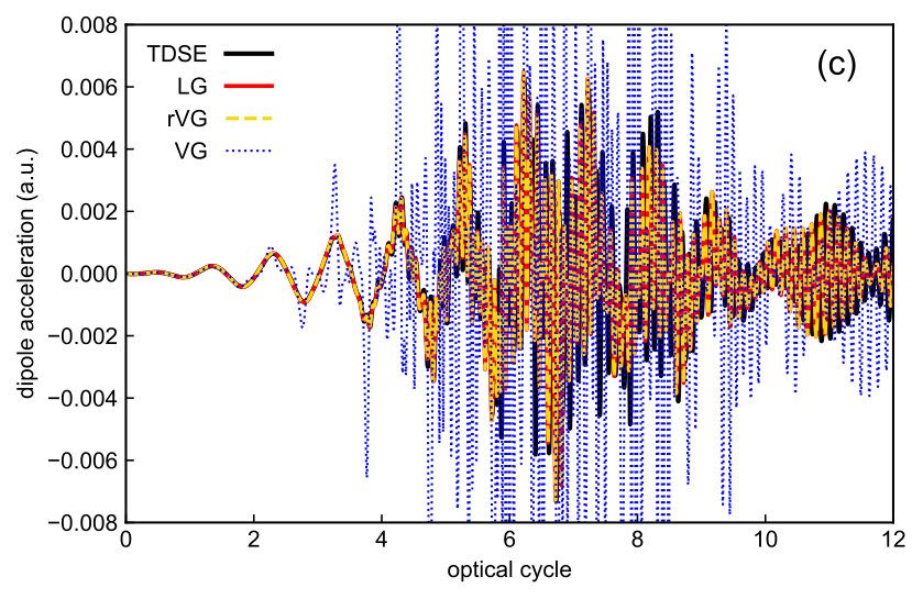 Figure 1
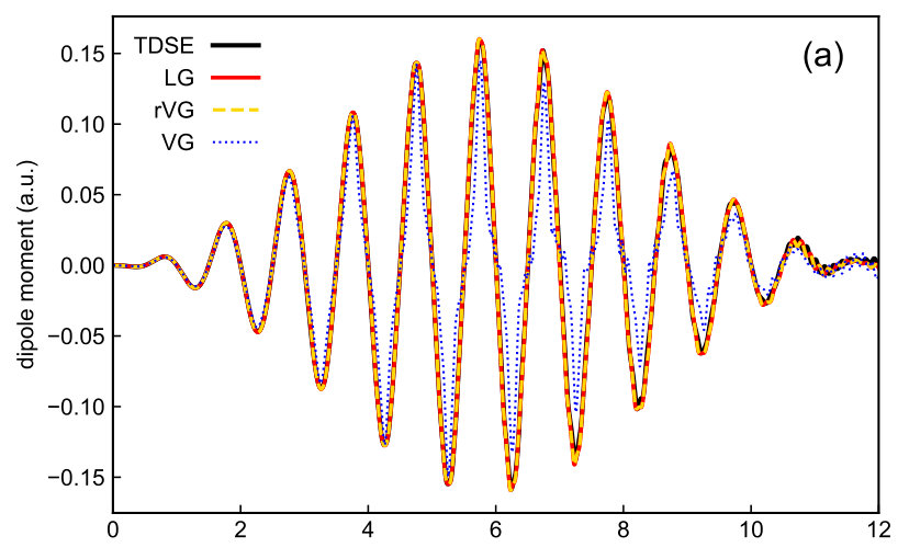 Figure 2
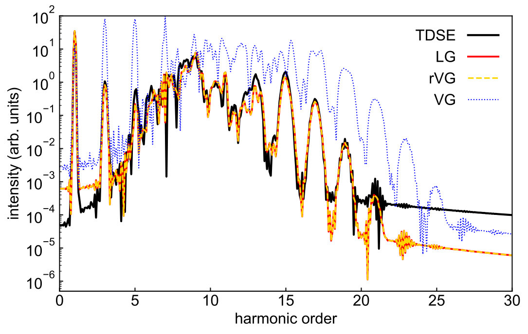 Figure 3
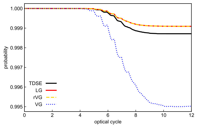 Figure 4
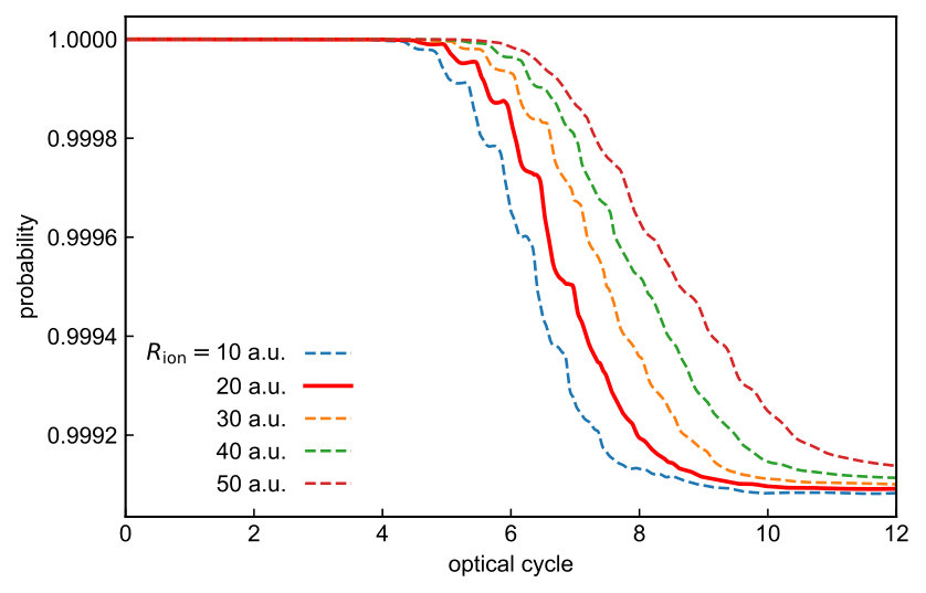 Figure 5
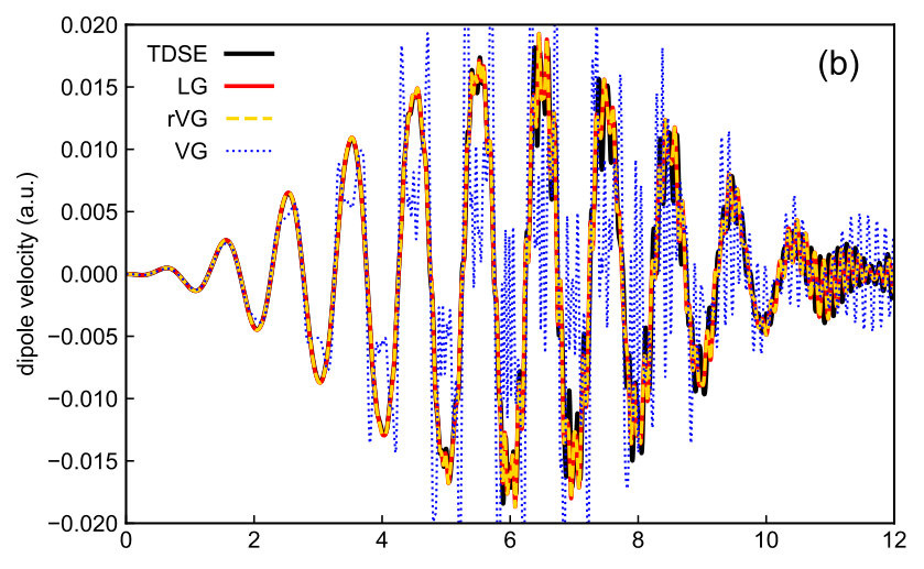 Figure 6
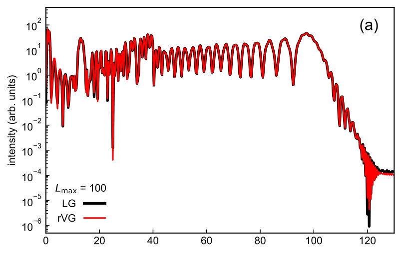 Figure 7
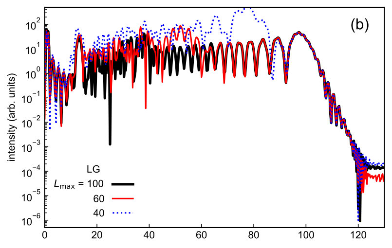 Figure 8
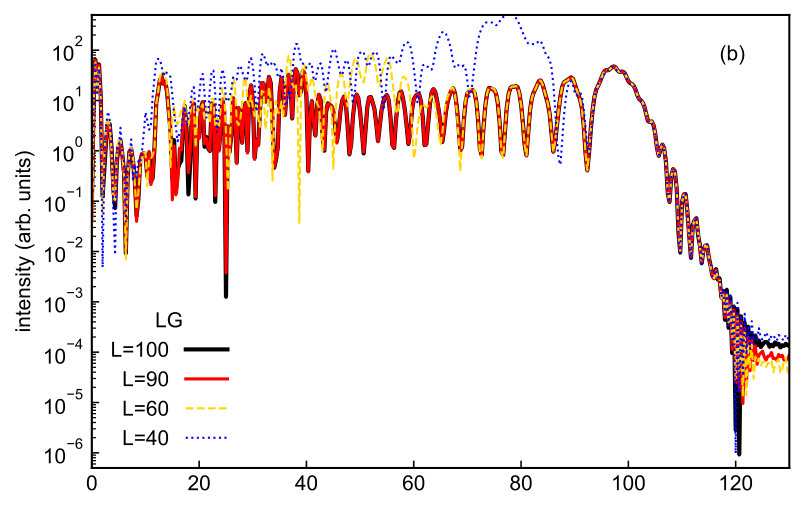 Figure 9
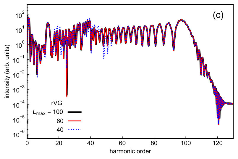 Figure 10
Peer Reviews
No public reviews on file for this paper yet. If you reviewed it on a platform where reviews are public (OpenReview, ICLR, NeurIPS, ICML), you can paste yours below so the community can read it here.
Videos
No videos yet. Explain this paper in a talk, walkthrough, or lecture? Add one.
Implementation of gauge-invariant time-dependent configuration interaction singles method for three-dimensional atoms
Takuma Teramura1
Takeshi Sato1,2,3
Kenichi L. Ishikawa1,2,3
1Department of Nuclear Engineering and Management, Graduate School of Engineering, The University of Tokyo, 7-3-1 Hongo, Bunkyo-ku, Tokyo 113-8656, Japan
2Photon Science Center, Graduate School of Engineering, The University of Tokyo, 7-3-1 Hongo, Bunkyo-ku, Tokyo 113-8656, Japan
3Research Institute for Photon Science and Laser Technology, The University of Tokyo, 7-3-1 Hongo, Bunkyo-ku, Tokyo 113-0033, Japan
Abstract
We present a numerical implementation of the gauge-invariant time-dependent configuration interaction singles (TDCIS) method [Appl. Sci. 8, 433 (2018)] for three-dimensional atoms. In our implementation, orbital-like quantity called channel orbital [Phys. Rev. A 74, 043420 (2006)] is propagated instead of configuration-interaction (CI) coefficients, which removes a computational bottleneck of explicitly calculating and storing numerous virtual orbitals. Furthermore, besides its physical consistency, the gauge-invariant formulation allows to take advantages of the velocity gauge treatment of the laser-electron interaction over the length gauge one in the simulation of high-field phenomena. We apply the present implementation to high-harmonic generation from helium and neon atoms, and numerically confirms the gauge invariance and demonstrates the effectiveness of the rotated velocity gauge treatment.
††preprint: APS/123-QED
I Introduction
Recent laser technology capable of generating strong laser pulses with an intensity has enabled us to explore electron dynamics in nonperturbative regime, e.g., high-harmonic generation (HHG), above threshold ionization, nonsequential double ionization, and attosecond pulse generation Krausz and Ivanov (2009); Nisoli et al. (2017); Gallmann et al. (2013). While laser-driven electron dynamics is rigorously described by the time-dependent Schrödinger equation (TDSE), its direct numerical solution is practically unfeasible for systems with more than two electrons. For theoretical investigation of multielectron dynamics in intense laser field, various tractable ab-initio methods have been developed, e.g., time-dependent multiconfiguration self-consistent field (TD-MCSCF) methods Zanghellini et al. (2003); Kato and Kono (2004); Haxton and McCurdy (2015a); Miyagi and Madsen (2014a); Caillat et al. (2005); Miyagi and Madsen (2013a, b); Sato and Ishikawa (2013); Miyagi and Madsen (2014b); Haxton and McCurdy (2015b); Sato and Ishikawa (2015); Sato et al. (2016); Anzaki et al. (2017), time-dependent coupled cluster method Kvaal (2012); Sato et al. (2018a), time-dependent matrix approach Lysaght et al. (2009, 2008); Burke and Burke (1997); Moore et al. (2011); Clarke et al. (2018), and time-dependent reduced two body density matrix approachLackner et al. (2015, 2017).
Among them, the time-dependent configuration interaction singles (TDCIS) method is one of the promissing methods Rohringer et al. (2006); Gordon et al. (2006); Karamatskou and Santra (2017); Pabst et al. (2011); Greenman et al. (2010); Grosser et al. (2017); Pabst and Santra (2014); Sytcheva et al. (2012); Pabst et al. (2012); Pabst and Santra (2013); Heinrich-Josties et al. (2014). This method has been successfully applied to various electron dynamics such as giant enhancement in HHG in Xe Pabst and Santra (2013) and decoherence in attosecond photoionization Gordon et al. (2006). In the TDCIS method, the total electronic wavefunction is approximated by a superposition of time-independent Slater determinants
[TABLE]
where is the Hartree-Fock (HF) ground state and is a singly-excited configuration replacing an occupied orbital with a virtual orbital unoccupied in the ground state. The orbital functions are fixed and propagation of configuration-interaction (CI) coefficients ( and) describes the system dynamics. Although applications of the TDCIS method are limited to the single excitation or ionization due to the truncation of CI space, its low computational cost and ease of analysis are attractive.
The conventional TDCIS method with CI coefficients has two major issues; the explicit calculation and storage of virtual orbitals and a violation of gauge invariance. Virtual orbitals should include both bound and continuum orbitals, whose number is infinite in principle. In a practical simulation with real-space grids, one has to prepare virtual orbitals in advance by numerically obtaining all eigenstates of the discretized HF equation. The number of the virtual orbitals increases with the number of the grid points. Thus, the calculation and storage of virtual orbitals become unacceptably demanding for systems with a large number of grid points like molecules. To solve this problem, Rohringer et.al. have proposed an alternative but equivalent formulation of the TDCIS method in which time-dependent orbital-like quantity called channel orbital is propagated instead of CI coefficient Rohringer et al. (2006). The channel orbital is defined by using and as
[TABLE]
The equations of motions (EOMs) of CI coefficient are converted to those of and . This reformulation removes computational bottleneck of handling numerous virtual orbitals, while in princple including all the virtual orbitals within a grid space, and has enhanced utility of the TDCIS method. However, to the best of our knowledge, the applications of the channel orbital-based TDCIS method have been limited to one-dimensional (1D) model in Refs. Rohringer et al. (2006); You et al. (2017, 2016) and nobles gas atoms with Hartree-Slater potential in Ref. Gordon et al. (2006).
The TDCIS method, either CI coefficient-based or channel-orbital-based, suffers from a violation of gauge invariance, as a general consequence of the truncation of CI space. Although it is known that the velocity gauge (VG) offers efficient simulations of high-field phenomena, it was impossible to enjoy this advantage within the TDCIS method. To overcome this difficulty, we have recently reported a gauge-invariant reformulation of the TDCIS method Sato et al. (2018b). In our reformulation, a rotated velocity gauge (rVG) transformed from the length gauge (LG) by a unitary operator has been introduced. This unitary transformation ensures the gauge invariance between the LG and rVG, and Ref. Sato et al. (2018b) numerically confirmed the equivalence of these gauges for a model 1D Hamiltonian.
In this paper, we report a three dimensional numerical implementation of the gauge-invariant TDCIS method for atoms subject to a linearly polarized laser pulse. We employ a spherical harmonics expansion of orbital functions with the radial coordinate discretized by a finite-element discrete variable representation (FEDVR)Rescigno and McCurdy (2000); McCurdy et al. (2004); Schneider et al. (2006, 2011). We apply the present implementation to HHG from helium and neon atoms and asses the advantage of the rVG over the LG and VG.
This paper proceeds as follows. In Sec. II, we briefly review the TDCIS methods. The numerical implementation of the gauge-invariant TDCIS method to three-dimensional atoms is given in Sec. III. We describe numerical applications in Sec. IV and conclude this work in Sec. V. We use Hartree atomic units (a.u.) throughout the paper unless otherwise stated.
II Theory
II.1 The System Hamiltonian and Gauge transformation
We consider an atom with electrons with a nucleus located at the origin. The time evolution of the -electron wavefunction is governed by the TDSE,
[TABLE]
where is the time-dependent non-relativistic Hamiltonian
[TABLE]
decomposed into the field-free part,
[TABLE]
and the laser-electron interaction part
[TABLE]
In these expressions, and are the position and the canonical momentum of the electron , respectively. is given by,
[TABLE]
where is the atomic number. Within the electric dipole approximation, for the LG and VG are given by
[TABLE]
where and are the electric field and the vector potential of the external laser field, respectively.
The two gauges are physically equivalent, and any physical observable takes the same value, independent of the choice of the gauge. The LG wavefunction and VG wavefunction are mutually transformed by a gauge transformation as,
[TABLE]
II.2 The CI coefficient-based TDCIS method in the length gauge
In the conventional TDCIS method based on CI coefficients, orbitals satisfy the canonical, restricted HF equation
[TABLE]
where is the Fock operator and is the potential due to the product of two given orbitals and , defined in the real space as
[TABLE]
is the orbital energy of orbital . In the TDCIS wavefunction in Eq. (1), is the HF ground state formed with the occupied orbitals as
[TABLE]
where and are the creation and annihilation operators, respectively, of spin-orbital , and is the vacuum. denotes the spin function. is a singly-excited configuration replacing an occupied orbital with a virtual orbital
[TABLE]
The EOMs of CI coefficients is derived through the Dirac-Frenkel time-dependent variational principle Kramer and Saraceno (1981), requiring Lagrangian
[TABLE]
to be stationary with respect to the variation of and . denotes the HF energy. This constant shift, introduced for the simple notation of the EOMs, does not affect physical results. In the LG case, in which the wavefuntion is written as,
[TABLE]
the EOMs of CI coefficients are obtained as
[TABLE]
where
[TABLE]
II.3 The channel orbital-based TDCIS method in the length gauge
The EOMs of CI coefficients [Eq. (17)] can be rewritten, by substituting channel orbital Eq. (2) into Eq. (17), as,
[TABLE]
where
[TABLE]
and is the projection operator onto the space spanned by virtual orbitals
[TABLE]
with being the identity operator.
II.4 Velocity gauge and rotated velocity gauge
One can, in principle, derive the EOMs for the VG case in the same way as for the LG. Let us write the total wavefunction and channel orbital as,
[TABLE]
and are the same configurations as those used in the LG case. Their EOMs are obtained through the same procedures as in the LG case as,
[TABLE]
It is known that TDCIS, which uses time-independent orbitals, is not gauge-invariant Ishikawa and Sato (2015); Sato et al. (2018b, c). Instead of the conventional VG as described above, we have recently proposed the rVG Sato et al. (2018b), where we define the rVG wavefunction by the gauge transformation from the LG wavefunction as,
[TABLE]
The rVG orbitals are related to the LG ones by,
[TABLE]
where
[TABLE]
They satisfy the following EOMs Sato et al. (2018b):
[TABLE]
where and are given by Eqs. (21) and (20), respectively, with replaced with . Although Eq. (29) contains the dipole operator , this does not prevent enjoying the advantages of the VG treatment, since it acts only on the localized occupied orbitals .
III Implementation to three-dimensional atoms
III.1 Spherical-FEDVR basis
The present implementation is based on our TD-MCSCF code Sato et al. (2016), which uses spherical-FEDVR basis functions
[TABLE]
where and are the radial and angular coordinate of , respectively, are spherical harmonics, and are radial FEDVR basis functions Rescigno and McCurdy (2000); McCurdy et al. (2004). The radial coordinate of the simulation box is divided into finite elements. Each finite element supports local DVR functions, and neighboring elements are connected by a bridge function. In total, there are radial grid points , on which with being the integration weights.
We expand the channel orbital in the spherical-FEDVR basis as
[TABLE]
where is the maximum angular momentum included. The FEDVR basis functions corresponding to and are removed to enforce the vanishing boundary condition for at both ends of the simulation box.
The electrostatic potentials for electron-electron interaction, and required for the EOM of channel orbitals, are computed by solving Poisson’s equation,
[TABLE]
using the method described in Ref. Sato et al. (2016). It should be noted that is time independent, and Eq. (32a) needs to be solved only once before the simulation. On the other hand, is time dependent, and should be computed at every time step. However, since its source [See Eq. (32b).] and operand [See Eq. (20)] are both localized around the atom due to the locality of occupied orbitals, Eq. (32b) can be solved with less computational cost than the similar equation appearing, e.g, in time-dependent Hartree-Fock and TD-MCSCF method Sato et al. (2016).
III.2 Time-propagation with exponential time differencing fourth-order Runge-Kutta scheme
For an efficient propagation of the EOM of channel-orbital based TDCIS, we use the exponential time differencing fourth-order Runge-Kutta scheme (ETDRK4) by Krogstad Krogstad (2005); Hochbruck and Ostermann (2010); Kidd et al. (2017). To this end, we arrange and into a unified vector and rewrite the EOMs of and by a matrix form
[TABLE]
where is a chosen stiff part of the right-hand side of the EOM (See below), and is a nonstiff remainder. We choose the stiff part to be either (i) the field-free one-electron Hamiltonian or (ii) the totality of the one-electron Hamiltonian . For the first case (i) with time-independent , the time propagation from to is given by
[TABLE]
where , , and are defined as
[TABLE]
where , , and
[TABLE]
, , , and are given by
[TABLE]
where , , and are intermediate vectors given as
[TABLE]
The operator exponential and in the spherical-FEDVR basis are approximated by the Padé (3/3) approximation, and higher-order functions are obtained by successively applying Eq. (36). The denominator of the Padé approximation is factorized and operated by the matrix iteration method Sato et al. (2016). We follow Ref. Hochbruck and Ostermann (2010) for the modification required for a time-dependent stiff part . In the absence of linear part for , time-propagation of reduces to well-known fourth-order Runge-Kutta scheme.
III.3 Expectation value
The expectation value of one-body operator can be evaluated in the LG case as Rohringer et al. (2006); Sato et al. (2018b)
[TABLE]
The VG expression is obtained by simply replacing with , and the rVG one by replacing with . The Ehrenfest theorem does not hold for TDCIS. Instead, we evaluate the time derivative of as Sato et al. (2018b),
[TABLE]
in the LG case. is to be replaced with for VG. The rVG case needs extra terms Sato et al. (2018b):
[TABLE]
Equations (39), (40), and (III.3) are valid not only for atoms but also any multielectron system including molecules.
III.4 Ionization probability
To conveniently analyze how ionization proceeds using the TD-MCSCF wavefunctions with time-varying orbitals, we have previously introduced Sato and Ishikawa (2013) a domain-based -fold ionization probability , defined as a probability to find electrons in the outer region and the other electrons in the inner region with a given distance from the origin. This quantity is gauge-invariant even during the pulse, unlike the population of the (field-free) continuum levels Ishikawa and Sato (2015); Sato et al. (2018c). To apply this approach to the TDCIS method with channel orbitals, it is reasonable to assume that the occupied orbitals are localized inside the inner region, i.e, for . Then, the yield of the neutral species, or the survival probability is computed as,
[TABLE]
where is the overlap integral in the inner region
[TABLE]
Noting that the atom described by a TDCIS wavefunction is at most singly ionized, we obtain the single-ionization probability as .
IV numerical example
We present numerical applications of the implementation of the reformulated TDCIS method described in the previous section and assess efficiency of the rVG. In all simulations reported below, we assume a laser field linearly polarized along the axis of the following form:
[TABLE]
where is the peak intensity, is the central frequency, is the period, and is the total number of optical cycles.
IV.1 Helium
First, we consider helium atom exposed to a laser pulse with , , and . In this condition, exact numerical solution of the TDSE is available Feist et al. (2009); Pazourek et al. (2011), from which the expectation value of dipole velocity and dipole acceleration can be calculated by using the Ehrenfest theorem. For the TDCIS method, we apply in Eqs. (39) and (40) to evaluate the expectation value of dipole moment and velocity, respectively. Dipole acceleration is computed by numerically differentiating dipole velocity.
Time evolution of the calculated dipole moment, dipole velocity, and dipole acceleration are shown in Fig. 1, and HHG spectra obtained as the modulus squared of the Fourier transform of the dipole acceleration is presented in Fig 2. In these figures, one can see the perfect agreement between the LG and rVG results, which numerically confirms the gauge invariance between the two gauges. In contrast, the results of conventional VG with fixed orbitals strongly deviate from them. It should be noted that, from the comparison between LG (and rVG) and VG results alone, we cannot a priori tell which is more accurate. The comparison with the TDSE results now reveals that the former reproduces the TDSE results much better than the latter, which convinces us of an empirical preference of the LG and rVG treatments.
We show the temporal evolution of the survival probability with a.u. in Fig. 3 (See Appendix for the dependence of ). The conventional VG treatment strongly overestimates ionization. Recalling that tunneling ionization is the first process of the three-step model Corkum (1993); Piraux et al. (1993), this explains the substantial overestimation of the HHG yield in Fig. 2. The LG and rVG results, on the other hand, underestimate tunneling ionization. Correspondingly, indeed, we notice that the harmonic intensity is slightly underestimated in Fig. 2.
IV.2 Neon
We next consider a neon atom subject to a laser field with 800 nm, W/cm2, and and discuss convergence with respect to the maximum angular momentum . We show the HHG spectra calculated with various values of in the LG and rVG in Fig. 4.
Figure 4. (a) shows the equivalence between the LG and rVG for sufficiently large . As can be seen in Fig. 4. (b), which shows LG results, is not sufficient to obtain a converged result. On the other hand, the rVG requires far less ; even well reproduces the result with , and the spectrum is converged with [Fig. 4. (c)]. This observation indicates that the rVG TDCIS is simultaneously as accurate as the LG and as efficient as the VG.
V conclusions
We have presented a 3D numerical implementation of the recently formulated gauge-invariant TDCIS method Sato et al. (2018b) for atoms subject to a linearly polarized intense laser field. Compared to the conventional TDCIS method that uses CI coefficients as working variables, the present implementation introduces channel orbitals Rohringer et al. (2006), avoiding calculation and storage of numerous virtual orbitals. We have applied this to He and Ne atoms, and calculated survival probabilities and HHG spectra for intense laser pulses. The perfect agreement of the LG and rVG results obtained with a sufficiently large number of partial waves numerically demonstrates the gauge invariance of the method. The comparison with the numerically exact TDSE results for He shows the rVG and LG’s superiority to the conventional VG in terms of accuracy. The VG largely overestimates tunneling ionization and, then, harmonic intensity. The analysis with neon reveals that the rVG has advantage in computational efficiency over the LG in terms of the number of spherical harmonics required to obtain converged HHG spectrum. Thus, our gauge-invariant reformulation will make TDCIS a promising approach for multielectron dynamics not only in atoms but also in molecules driven by high-intensity laser fields.
acknowledgments
We are grateful to Prof. J. Burgdörfer of Vienna University of Technology for providing us with He TDSE benchmark results. This research was supported in part by a Grant-in-Aid for Scientific Research (Grants No. 16H03881, No. 17K05070, No. 18H03891, and No. 19H00869) from the Ministry of Education, Culture, Sports, Science and Technology (MEXT) of Japan. This research was also partially supported by JST COI (Grant No. JPMJCE1313), JST CREST (Grant No. JPMJCR15N1), and by Quantum Leap Flagship Program of MEXT. T. T. gratefully acknowledges support from the Graduate School of Engineering, The University of Tokyo, Doctoral Student Special Incentives Program (SEUT Fellowship).
Appendix A dependence on
We show from the LG TDCIS results with various values of in fig. 5. We can see stepwise ejection of electron wavepackets that propagate outwards; the larger is, the later is depleted. In the cases of 10, 20, and 30 a.u., nearly reaches approximately the same final value in the end of the simlation (after twelve optical cycles).
The reference list from the paper itself. Each links out to its DOI / PubMed record.
- 1Krausz and Ivanov (2009) F. Krausz and M. Ivanov, Rev. Mod. Phys. 81 , 163 (2009) . · doi ↗
- 2Nisoli et al. (2017) M. Nisoli, P. Decleva, F. Calegari, A. Palacios, and F. Martín, Chem. Rev. 117 , 10760 (2017) . · doi ↗
- 3Gallmann et al. (2013) L. Gallmann, C. Cirelli, and U. Keller, Annu. Rev. Phys. Chem. 63 , 447 (2013).
- 4Zanghellini et al. (2003) J. Zanghellini, M. Kitzler, C. Fabian, T. Brabec, and A. Scrinzi, Laser Phys. 13 , 1064 (2003) .
- 5Kato and Kono (2004) T. Kato and H. Kono, Chem. Phys. Lett. 392 , 533 (2004) . · doi ↗
- 6Haxton and Mc Curdy (2015 a) D. J. Haxton and C. W. Mc Curdy, Phys. Rev. A 91 , 012509 (2015 a) . · doi ↗
- 7Miyagi and Madsen (2014 a) H. Miyagi and L. B. Madsen, Phys. Rev. A 89 , 063416 (2014 a) . · doi ↗
- 8Caillat et al. (2005) J. Caillat, J. Zanghellini, M. Kitzler, O. Koch, W. Kreuzer, and A. Scrinzi, Phys. Rev. A 71 , 012712 (2005) . · doi ↗