On the numerical experiments of the Cauchy problem for semi-linear Klein-Gordon equations in the de Sitter spacetime
Takuya Tsuchiya, Makoto Nakamura

TL;DR
This paper presents numerical experiments analyzing the long-term behavior of solutions to semi-linear Klein-Gordon equations in de Sitter spacetime, highlighting the effects of the Hubble constant and the importance of structure-preserving schemes.
Contribution
It introduces a structure-preserving numerical scheme for simulating the equations and demonstrates its effectiveness in capturing long-term dynamics and diffusion effects.
Findings
Large Hubble constant induces strong diffusion effects.
The scheme preserves the numerically modified Hamiltonian.
Simulations show stable, long-term behavior of solutions.
Abstract
The computational analysis of the Cauchy problem for semi-linear Klein-Gordon equations in the de Sitter spacetime is considered. Several simulations are performed to show the time-global behaviors of the solutions of the equations in the spacetime based on the structure-preserving scheme. It is remarked that the sufficiently large Hubble constant yields the strong diffusion-effect which gives the long and stable simulations for the defocusing semi-linear terms. The reliability of the simulations is confirmed by the preservation of the numerically modified Hamiltonian of the equations.
Click any figure to enlarge with its caption.
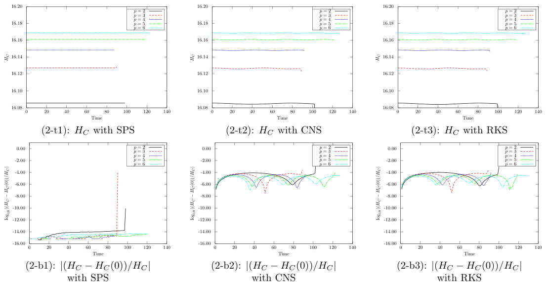 Figure 0
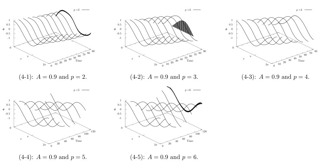 Figure 0
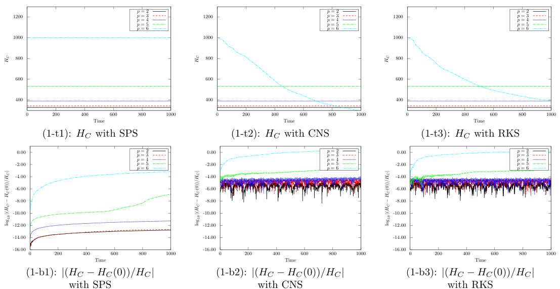 Figure 0
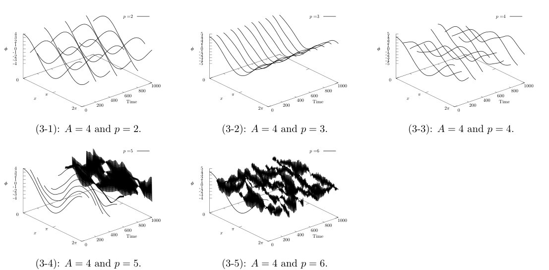 Figure 0
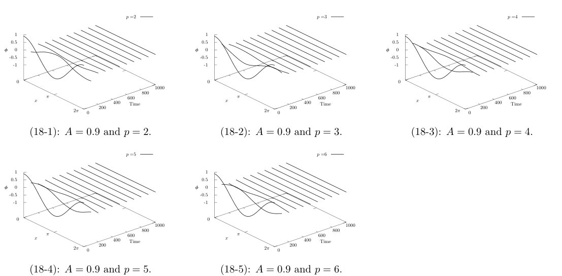 Figure 2
 Figure 2
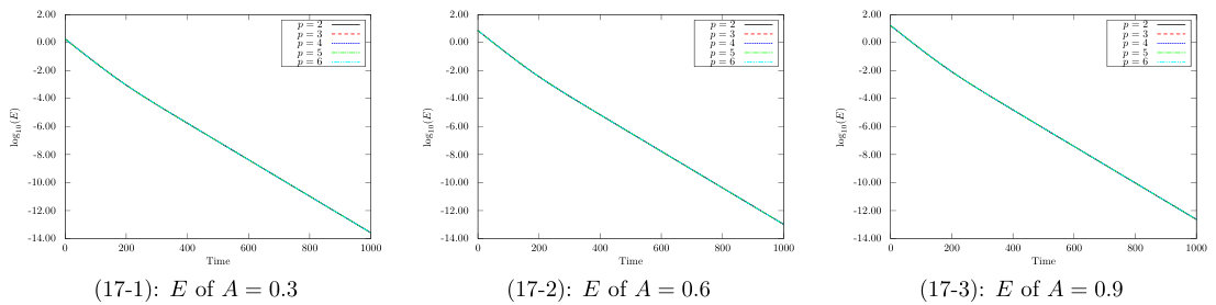 Figure 2
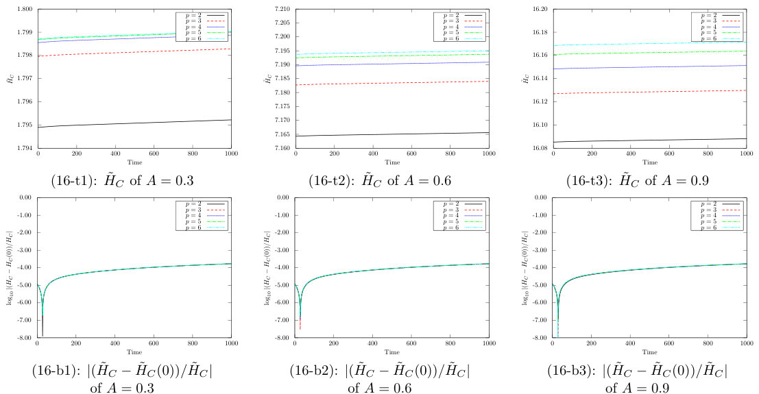 Figure 2
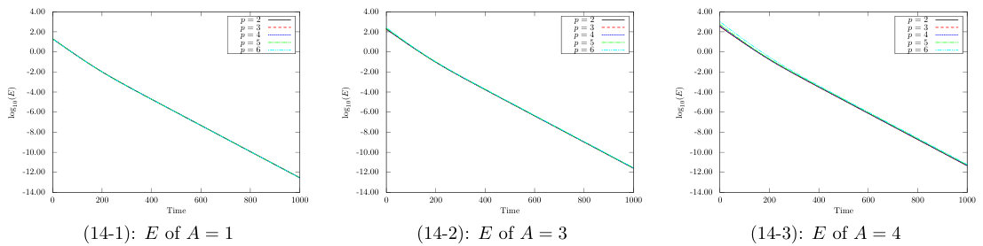 Figure 2
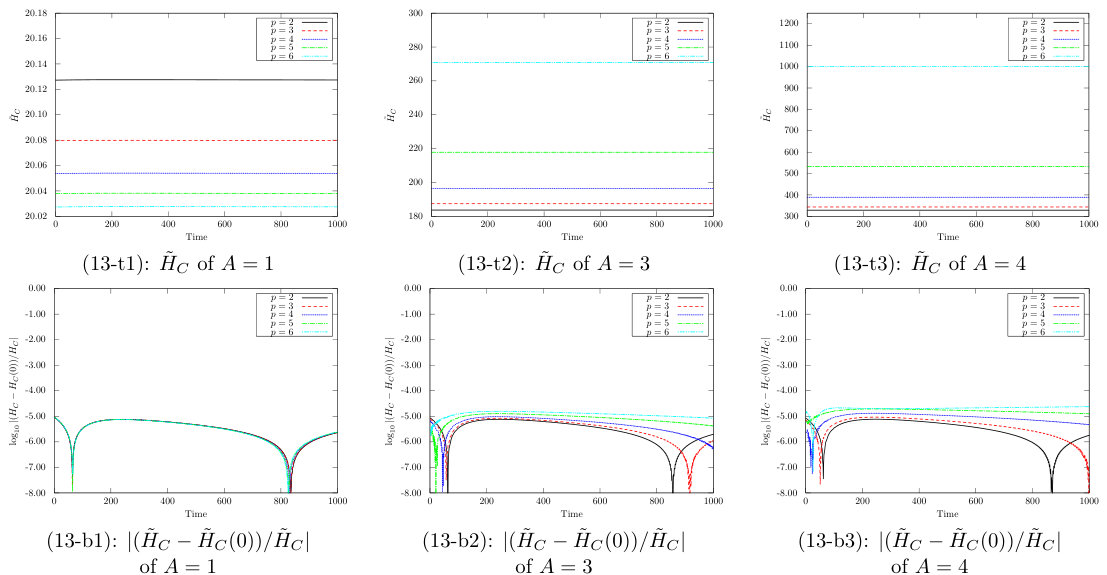 Figure 2
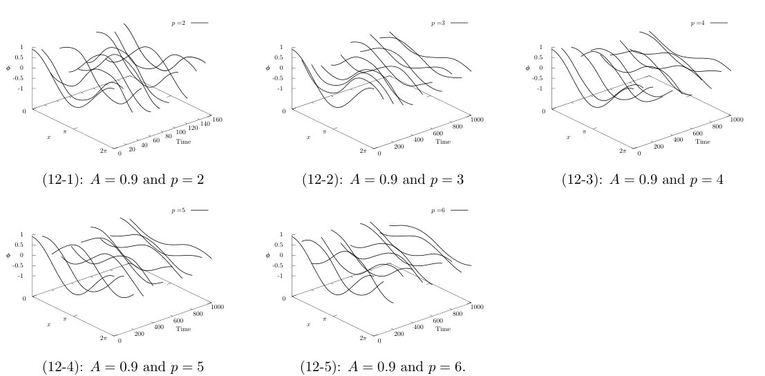 Figure 3
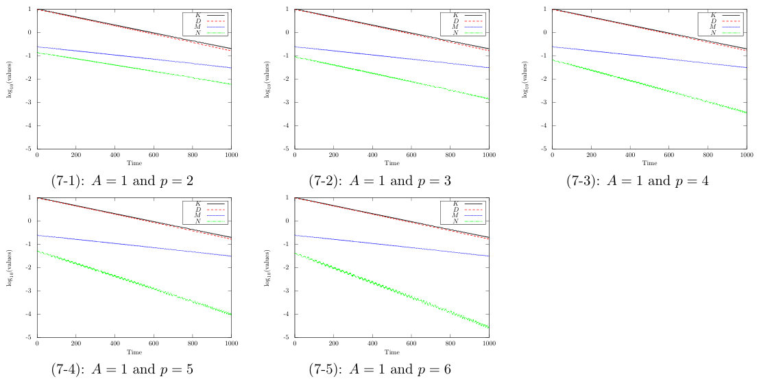 Figure 3
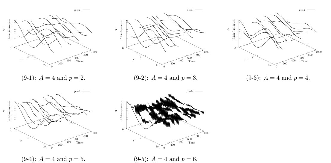 Figure 3
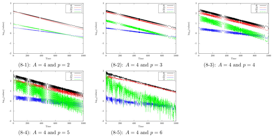 Figure 3
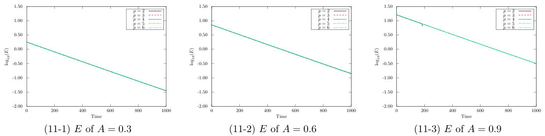 Figure 3
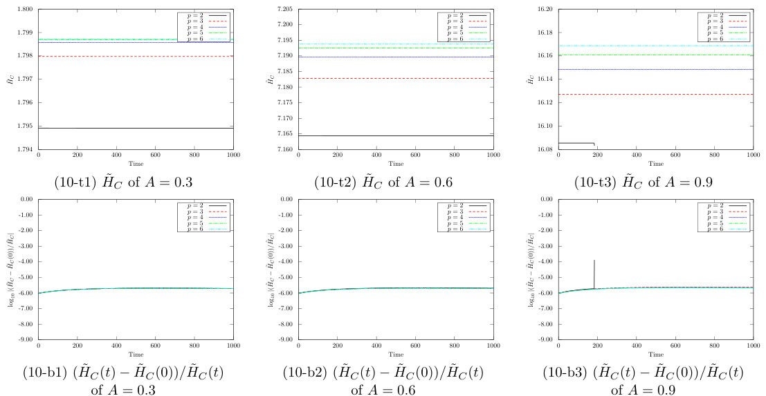 Figure 3
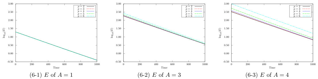 Figure 3
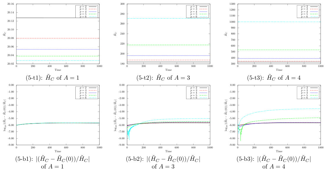 Figure 3
Peer Reviews
No public reviews on file for this paper yet. If you reviewed it on a platform where reviews are public (OpenReview, ICLR, NeurIPS, ICML), you can paste yours below so the community can read it here.
Videos
No videos yet. Explain this paper in a talk, walkthrough, or lecture? Add one.
On the numerical experiments
of the Cauchy problem for semi-linear Klein-Gordon equations in the de Sitter spacetime
Takuya Tsuchiya
Makoto Nakamura
Center for Liberal Arts and Sciences, Hachinohe Institute of Technology, 88-1, Obiraki, Myo, Hachinohe, Aomori 031-0814, JAPAN.
Faculty of Science, Yamagata University, Kojirakawa-machi 1-4-12, Yamagata 990-8560, JAPAN.
Abstract
The computational analysis of the Cauchy problem for semi-linear Klein-Gordon equations in the de Sitter spacetime is considered. Several simulations are performed to show the time-global behaviors of the solutions of the equations in the spacetime based on the structure-preserving scheme. It is remarked that the sufficiently large Hubble constant yields the strong diffusion-effect which gives the long and stable simulations for the defocusing semi-linear terms. The reliability of the simulations is confirmed by the preservation of the numerically modified Hamiltonian of the equations.
keywords:
semilinear Klein-Gordon equation , Cauchy problem , de Sitter spacetime , structure-preserving scheme
MSC:
[2010] 65M99 , 35L70 , 35Q75
††journal: Journal of Computational and Applied Mathematics
1 Introduction
The mathematical structure of partial differential equations in non-flat spacetimes is changed by the variations of curvatures since the differential operators are influenced by the metrics of the spacetimes. The de Sitter spacetime is one of the solutions of the Einstein gravitational equations with the cosmological constant in the vacuum. The space is expanding or contracting along the time in this spacetime. To study the effects of the spatial variation, we consider the semilinear field equation of the Klein-Gordon type, and we carry out the numerical experiments of the solutions and their energy. To investigate the partial differential equations with computational analysis, we need to perform high precise and accurate simulations. There are many methods to make discretized equations.
The Adomian decomposition method [1] can provide analytical approximation solutions of linear and nonlinear differential equations. Since this method dose not require the linearization, it would be appropriate to make dicretization of the nonlinear differential equations. It is reported that the simulations of the nonlinear Klein-Gordon equation in the flat spacetime with the method [5]. In [31], the differential transform method [32] and the variational iteration method [24] are used to perform the nonlinear Klein-Gordon equation in the de Sitter spacetime. The former is one of the power series expansions. The virtue is easy to estimate the numerical errors because the truncation higher order terms are corresponding to the dominant numerical errors. Since the latter is classified as the method of Lagrange multipliers, it would be close to the exact solutions by repeating the iteration if the appropriate conditions are given. In addition, the results with the explicit fourth-order Runge-Kutta method are reported in [4]. The Runge-Kutta method is well-known discretized scheme for the nonlinear differential equations.
The above methods are generic discretization schemes for the differential equations to calculate simulations. Therefore, the properties of the differential equations in continuous level often lost in the discretization, and it makes the numerical errors in the evolutions. On the other hand, we use the structure-preserving scheme (SPS) called as “discrete variational derivative method” in this paper. The concept of this method is to conserve the structures and the properties of the equations in continuous level. This method is widely used to derive the discrete equations of partial differential equations (see e.g., [8, 9, 22]). To make discretized equations using SPS, we need the Lagrangian or the Hamiltonian[12, 25]. This is because the derivations of the discretized equations with SPS are similar with the process of making the continuous equations using the variational principle. In comparison with the construction of the Lagrangian formulation, the one of the Hamiltonian formulation is clear. Especially, since the Hamiltonian means the total energy of the system, this value is regarded as one of the constraints of the system. By monitoring the value in the evolution, we can judge whether the numerical simulations are success or not. Conservation of the constraints is one of the necessary conditions to perform successive simulations. If the constraints dose not conserve in the evolution, the simulations fail (e.g. [21]). Therefore, we use the Hamiltonian formulation in this paper.
We start from the introduction of the de Sitter spacetime. Let be the spatial dimension, be the speed of light. In the following, Greek letters run from [math] to , Latin letters run from to . Let be the metric in . We denote by the -matrix whose -component is given by . Put , and let be the inverse matrix of . We use the Einstein rule for the sum of indices of the tensors, for example, and . The change of upper and lower indices of the tensors is done by and , for example, .
For a stress-energy tensor , the -dimensional Einstein equation is defined by
[TABLE]
where is the Einstein tensor, is the cosmological constant, and is the Einstein gravitational constant. When we consider the universe filled with the perfect fluid of the mass density and the pressure , we are able to use the stress-energy tensor of the perfect fluid given by
[TABLE]
When the cosmological term is transposed to right-hand-side in (1.1), the term is regarded as a part of the stress-energy tensor. Then the term is rewritten as
[TABLE]
and the cosmological constant is regarded as the energy which has positive density and negative pressure. Thus, we regard the cosmological constant as “the dark energy.” The study of roles of the cosmological constant and the spatial variance is important to describe the history of the universe, especially, the inflation and the accelerating expansion of the universe (see e.g., [13], [14], [17], [18], [19], [20]). One of the solutions of the equation (1.1) is the de Sitter spacetime, and its line-element with the spatial zero-curvature is given by
[TABLE]
where , is the Hubble constant, and denotes the Kronecker delta. The relation between the cosmological constant and the Hubble constant is given by . We can write .
Next, we introduce the semilinear Klein-Gordon equation (KGE) in curved spacetimes. KGE presents the equation of motion for the massive scalar field. Then, to derive the equation of motion described by a real-valued function with the mass and the potential , we consider the Lagrangian density defined by
[TABLE]
where is the covariant derivative associated with and is the Planck constant. If the spacetime is flat, the Lagrangian density is consistent with the well-known Lagrangian density of KGE (see e.g., [25]). The Euler-Lagrange equation of the action gives KGE in curved spacetime
[TABLE]
In the de Sitter spacetime, KGE is rewritten as
[TABLE]
where denotes the derivative for (see, e.g., [7, 15, 26]). Multiplying to the both sides of (1.4), we have the divergence formula
[TABLE]
where , , and mean the energy density and the external energy, respectively. They are defined by
[TABLE]
We define the total energy by
[TABLE]
then we have the energy estimate
[TABLE]
for . Let us consider the defocusing potential (), by which is a positive-valued function for any non-trivial solution . When the space is expanding (), the estimate (1.6) shows the dissipative property for . On the other hand, when the space is contracting (), (1.6) shows the anti-dissipative property for .
We introduce the known theoretical results on KGE (1.4). Let us consider the scalar potential of power type and its derivative given by
[TABLE]
for and . We consider the Cauchy problem
[TABLE]
where , are given initial data, denotes the Sobolev space and denotes the Lebesgue space. On the Cauchy problem (1.8) for the positive Hubble constant , the following theoretical results have been shown. The first result shows the existence of the time-local solutions for any initial data. The second result shows that the local solutions are time-global solutions if the initial data are sufficiently small. The third result shows the local solutions are global for any data if the semilinear term is defocusing.
Theorem 1.1
([15, Theorems 1.2 and 1.7]) Let . Assume . Let satisfy
[TABLE]
Then we have the following results.
(1) For any and , there exists such that (1.8) has a unique solution in .
(2) Let . If is sufficiently small, and , then (1.8) has a unique solution in .
(3) If , then (1.8) has a unique global solution in for any data and .
We refer to the corresponding known results on (1.8). D’Ancona and Giuseppe have shown in [2] and [3] global classical solutions for with some additional conditions on and when . Yagdjian has shown in [28] small global solutions for (1.11) with arbitrary when the nonlinear term is of power type , and the norm of initial data is sufficiently small for some (see also [29] for the system of the equations). Galstian and Yagdjian has extended this result to the case of the Riemann metric space for each time slices in [11]. In [15], the energy solutions in Theorem 1.1 have been shown. This result has been extended to the case of general Friedmann-Lemaître-Robertson-Walker spacetime in [10]. Baskin has shown in [7] small global solution for when is a type of , , , , where gives the asymptotic de Sitter spacetime (see also [6] for the cases with , with ). Blow-up phenomena are considered in [27]. See also the references in the summary [30] by Yagdjian.
In Theorem 1.1, we have assumed the condition by the following reason. Since the first equation in (1.8) has the dissipative (or anti-dissipative) term , we use the transformation for to transform the equation to the Klein-Gordon equation. Then the equation is rewritten as
[TABLE]
and we obtain the equation
[TABLE]
when , . We assume is large such that (see [26]). Here, we expect some dissipative effects when in (1.10). However, is needed for the energy estimates for (1.11), and is needed for the contraction argument to show the existence of the solutions of (1.11). So that, we assume , by which we lose the dissipative term in (1.11). Since the first equation in (1.8) has the term with the non-constant coefficient, it is not easy to obtain the critical theoretical results so far. Instead, in this paper, we carry out some numerical simulations, and show the detailed behaviors to clarify the dissipative effect of the spatial expansion.
2 Hamiltonian formulation of KGE
Let us consider the Hamiltonian density for the Lagrangian density . The Lagrangian density of KGE (1.3) in the de Sitter spacetime becomes
[TABLE]
Then, we define the momentum by
[TABLE]
the Hamiltonian density by the Legendre transformation
[TABLE]
and the Hamiltonian by
[TABLE]
for . To investigate the properties of , we denote the kinetic term, the diffusion term, the mass term and the nonlinear term by the integration of , , and . Namely,
[TABLE]
for . With (2.7), the total energy (1.5) can be expressed as
[TABLE]
Since the relation between and the energy density becomes
[TABLE]
can be expressed as
[TABLE]
If the spacetime is flat () and the speed of light is set as 1, then is consistent with . The Hamiltonian formulation of (1.4) is given by the canonical equations
[TABLE]
Since satisfies the differential equation
[TABLE]
where we have put
[TABLE]
satisfies the equation
[TABLE]
and by using (2.7), (2.13) can be expressed as
[TABLE]
The equation (2.13) (or (2.14)) indicates is not conserved in time evolution if the Hubble constant is not zero. Therefore, we define as
[TABLE]
which is a constant value in time evolution independent of the value of .
The behaviors of and show the properties of the effects of the spatial expansion and contraction by the Hubble constant . Namely, we are able to understand the properties of the dark energy, which is equivalent to the cosmological constant mathematically, through the asymptotic behaviors of , and . However, it is not easy to obtain the detailed behaviors of them by theoretical methods since the waves of would be oscillating and interfered by the semilinear term , and (1.4) is the equation with the variable coefficient. Thus, we perform the numerical simulations on , and to study the detailed dissipative effects of the spatial expansion.
3 Discrete KGE
To investigate KGE by computational analysis, we need the high precise and accurate numerical data. Then, we use SPS to get the high precise and accurate numerical results. With this scheme, the structures of the equations in the continuous case are preserved in the discrete case. In this paper, we use this scheme to make the discrete Hamiltonian formulation. The discrete values of the variable are defined as , where is the time index, is the time mesh width, is the spatial grid index, and is the spatial mesh width. The details of this are in Ref.[9].
For comparison with SPS, we use the Crank-Nicolson scheme (CNS) and the fourth-order Runge-Kutta scheme (RKS) which are widely used for calculating partial differential equations numerically.
3.1 SPS
By using SPS, we can get a set of discrete evolution equations of KGE. We give a discrete Hamiltonian density as
[TABLE]
where presents the time of the th step and is the centered space operator defined by
[TABLE]
For , and , we define the values
[TABLE]
by the equation
[TABLE]
Then, a set of discrete KGE with SPS becomes
[TABLE]
The discrete evolution equations (3.9) are corresponding to (2.12) for the continuous case. The nonlinear term of the last term in (3.9) is expressed as
[TABLE]
when is a natural number. We refer to the expression in the nonlinear Schrödinger equations in Ref.[9] to make above relation. With (3.9), the time difference of is calculated as
[TABLE]
[TABLE]
[TABLE]
where we use the relation of . We define the discrete Hamiltonian by
[TABLE]
then (3.11) is calculated as
[TABLE]
where , , and are defined by
[TABLE]
, , and are discrete values corresponding to , , and defined by (2.7), respectively. We set
[TABLE]
then is a discretized value of defined by (2.15). This value is a guideline to perform precise numerical simulations in the cases of .
3.2 CNS and RKS
CNS and RKS are frequently used to perform partial differential equations. The discrete equations of (2.12) with CNS are given by
[TABLE]
where the right hand sides of (3.22) are defined as
[TABLE]
and the second-order central difference operator is defined as
[TABLE]
The discrete equations with RKS are give by
[TABLE]
where
[TABLE]
4 Numerical tests
In this section, we carry out the numerical simulations on , and (or ). Since the physical background of the Einstein equation is for the dimensional spacetime, we consider the case in the following.
The numerical settings are below. Set .
Initial condition:
[TABLE]
- 2.
Numerical domains: , .
- 3.
Boundary condition: periodic.
- 4.
Grids: , and .
- 5.
Physical settings: mass , speed of light , Planck constant .
- 6.
The number of exponent in the nonlinear term: .
We consider the solution for which is a constant along the variables and to give simple and reliable simulations. More general solutions and data will be considered in the future. We perform the simulations by changing the values of the amplitude in the initial condition, the coefficient value of the nonlinear term, and the Hubble constant . First, we perform some simulations to study the accuracies with SPS. For comparison with SPS, we use the Crank-Nicolson scheme (CNS) and the Runge-Kutta scheme (RKS) which are widely used for calculating partial differential equations numerically. Because of the nonlinearity of KGE (2.12), the discretized equations are calculated implicitly. Thus, the numerical simulations are performed iteratively. For SPS and CNS, the iterations are nine times and three times, respectively. If we calculate more times iteratively for each scheme, the numerical results become worse in our codes. For the wave equation
[TABLE]
with (1.7), namely, , in (1.4) with (1.7), the scaling argument for the solution for yields the critical exponent of for the well-posedness of the Cauchy problem of the equation in the Sobolev space for . Especially, is called the Fujita exponent, is called the conformal exponent, is called the energy critical exponent. This exponent also plays crucial roles for the Klein-Gordon equation, and it satisfies
[TABLE]
By the simulations for , we are able to know the behaviors of the solutions for which is equivalent or close to these critical exponents.
4.1 Case 1:
To compare with the numerical results of SPS, CNS and RKS, we set the Hubble constant as zero in this subsection. In this case, is consistent with , and is constant with time evolutions theoretically. To show the accuracy of the simulations, we monitor .
We draw , and the differences between and the initial value in the evolutions with SPS, CNS and RKS for and in Fig.1. From the bottom panels (1-b1)–(1-b3), we see the values of with CNS and RKS are larger than the ones with SPS.
Next, we show the results for and in Fig.2.
We see the simulations stop before . From the bottom panels, we see the values of with SPS are smaller than the ones with CNS and RKS. In comparison with Fig.2, the simulations in Fig.1 are robust. Since it is necessary condition of performing correct simulations that the value of is small, KGE have to be performed with SPS. Therefore, we use the numerical scheme as SPS hereafter.
The results of with SPS are shown in Fig.3 and Fig.4. Fig.3 shows the case of and . We see that the vibrations occur for . Fig.4 shows the case of and . We see all of the simulations stop before .
4.2 Case 2:
In this subsection and next subsection, we perform the numerical simulations for . First, we calculate for and . When , is not constant in time evolutions. Since we cannot judge the reliability of simulations by monitoring the values of , we show defined by (2.15) instead of .
Fig.5 shows , and the differences between and the initial value for . We see the value of is the largest and that of is the smallest in the panel (5-t1). Contrarily, in the others of the top panels we see the largest value is the case of . The reason is or not. If , the nonlinear term becomes small as becomes large. On the other hand, if , the value becomes large as becomes large. From the bottom panels (5-b1)–(5-b3), we see of the case is the largest of them in each panel but all of the values in the bottom panels are enough small.
Fig.6 shows the total energy defined by (1.5). We see that the energy is exponential decay. Furthermore, the slopes of the lines in the panels of the figure are almost the same. This result means the diffusion effect with time evolutions is not caused by changing in or . While the lines in Panel (6-1) which is the case of are almost overlapping, there are differences between the values of for . To investigate the reason, we show the components of defined by (2.7).
The kinetic term , the diffusion term , the mass term and the nonlinear term for are shown in Fig.7 and the ones for are in Fig.8. We see that and are the dominant terms, and and are very small compared with and in Fig.7. The decline of the energy-component is becoming faster than , and as the power increases. On the other hand, the proportion of to becomes large as becomes large in Fig.8. This is because there are the differences between s in Fig.6.
Fig.9 shows for and , and the numerical settings are the same as Fig.3 except for the value of . The vibrations occur in the only case of . Since the vibrations occur in the cases of in Fig.3, the Hubble constant seems to affect generations of the vibrations of .
Next we show the results of the simulations with the case of .
Fig.10 shows and for , and . While we see the simulation for and stops before in Panel (10-t3) and Panel (10-b3), the values for the other cases are enough small.
Fig.11 shows for , and . It seems there is no difference between the slopes of all the lines in Fig.6 and Fig.11 regardless of the values of , and . Thus, the dissipation effect of is not caused by changing in , and the signature of .
Fig.12 shows for , and . These results are the same as Fig.4 except for the value of . By comparing Fig.4 with Fig.12, the simulation times for are longer than that for . It means the Hubble constant would influence the stability of the simulation. By comparing Fig.9 and Fig.12, the simulations for are robust against the case of since the calculation time for and is short. The tendency is the same as the case of .
4.3 Case 3:
In this subsection, we perform some simulations with and .
Fig.13 shows and for and this figure is the same as Fig.5 except for the value of . We see all the values of for are enough small.
Fig.14 shows with the Hubble constant as . There are few differences between the changes of compared with the cases of in Fig.6. By comparing Fig.6 and Fig.14, the diffusion effect of for is stronger than that for . Thus, the diffusion effect is mainly caused by the Hubble constant, and the effect would become strong as becomes large.
In Fig.15 which shows for , we see the waveform is damped and there are few vibrations of the waveform. By comparing Fig.3, Fig.9 and Fig.15, the stability of the simulations becomes good as becomes large since the vibrations of decreases as becomes large.
Next we show the results for .
In Fig.16, we see the simulations are reliable since all of the values of are enough small.
Fig.17 shows the total energy . By comparing Fig.11 and Fig.17, we see the diffusion effect for and is stronger than that for and . Thus, considering the results for , the diffusion effect is mainly caused by not the signature of the nonlinear term but the Hubble constant.
Fig.18 shows for and . The simulation times become long as becomes large from the results in Fig.4, Fig.12 and Fig.18. These results indicate the simulations become stable as becomes large.
5 Concluding remark
In this paper, we made the Hamiltonian formulation of the semilinear Klein-Gordon equation, and we derived the discrete equation with the structure-preserving scheme (SPS). To show the reliability of the simulations, we proposed the constant value when the Hubble constant is zero case and when the Hubble constant is nonzero case. With SPS, the Crank-Nicolson scheme (CNS) and the Runge-Kutta scheme (RKS), we performed some simulations in flat spacetime. Then, we showed the superiority of SPS to CNS and RKS in some simulations. We performed some simulations with small and showed the influence of the Hubble constant on the numerical stability. Especially, if the signature of the nonlinear term is negative, the simulations stop in some cases. However, with the negative nonlinear term, we showed the enough large value of the Hubble constant gives the long and stable simulations. It is remarkable that the diffusion effect caused by the positive Hubble constant is much stronger than the nonlinear term. Thus, we conclude that we are able to perform stable simulations when the Hubble constant is a sufficiently large. While the diffusion effects are expected from the theoretical point of view since the equation (1.4) has the positive-dissipative term for the positive Hubble constant (), the case of the negative Hubble constant () seems to be unstable and requires more delicate consideration since the numerical errors must be rigorously estimated for the blow-up solutions in the unstable case, which will be reported in the subsequent paper.
Acknowledgements
This work was supported by JSPS KAKENHI Grant Number 16H03940 (M.N.).
The reference list from the paper itself. Each links out to its DOI / PubMed record.
- 1[1] G. Adomian, A review of the decomposition method in applied mathematics, J. Math. Anal. Appl. 135 (2) (1988) 501–544.
- 2[2] P. D’Ancona, A note on a theorem of Jörgens, Math. Z. 218 (1995) 239–252.
- 3[3] P. D’Ancona, A. Di Giuseppe, Global existence with large data for a nonlinear weakly hyperbolic equation, Math. Nachr. 231 (2001) 5–23.
- 4[4] A. Balogh, J. Banda, K. Yagdjian, High-performance implementation of a Runge-Kutta finite-difference scheme for the Higgs boson equation in the de Sitter spacetime, Commun. Nonlinear. Sci. Numer. Simul. 68 (2019) 15–30.
- 5[5] K.C. Basak, P.C. Ray, R.K. Bera, Solution of non-linear Klein-Gordon equation with a quadratic non-linear term by Adomian decomposition method Commun. Nonlinear. Sci. Numer. Simul. 14 (2009) 718–723.
- 6[6] D. Baskin, A Strichartz estimate for de Sitter space, The AMSI-ANU Workshop on Spectral Theory and Harmonic Analysis, 97–104, Proc. Centre Math. Appl. Austral. Nat. Univ., 44, Austral. Nat. Univ., Canberra, 2010.
- 7[7] D. Baskin, Strichartz Estimates on Asymptotically de Sitter Spaces, Annales Henri Poincaré 14 (2) (2013) 221–252.
- 8[8] D. Furihata, Finite difference schemes for ∂ u ∂ t = ( ∂ ∂ x ) α δ G δ u 𝑢 𝑡 superscript 𝑥 𝛼 𝛿 𝐺 𝛿 𝑢 \frac{\partial u}{\partial t}=\left(\frac{\partial}{\partial x}\right)^{\alpha}\frac{\delta G}{\delta u} that inherit energy conservation or dissipation property, J. Comput. Phys. 156 (1999) 181–205.