Intrinsic and Dual Volume Deviations of Convex Bodies and Polytopes
Florian Besau, Steven Hoehner, Gil Kur

TL;DR
This paper investigates the asymptotic approximation of the Euclidean ball by polytopes using intrinsic and dual volume-based distances, providing sharp bounds and identifying nearly optimal polytopes in high dimensions.
Contribution
It introduces new notions of distance between convex bodies based on intrinsic and dual volumes and derives asymptotically sharp bounds for high-dimensional approximation.
Findings
Established asymptotic bounds for approximation by polytopes using intrinsic volumes.
Identified a polytope nearly optimal for all intrinsic volumes simultaneously.
Derived asymptotic formulas for approximation using dual volumes from Lutwak's theory.
Abstract
We establish estimates for the asymptotic best approximation of the Euclidean unit ball by polytopes under a notion of distance induced by the intrinsic volumes. We also introduce a notion of distance between convex bodies that is induced by the Wills functional, and apply it to derive asymptotically sharp bounds for approximating the ball in high dimensions. Remarkably, it turns out that there is a polytope which is almost optimal with respect to all intrinsic volumes simultaneously, up to absolute constants. Finally, we establish asymptotic formulas for the best approximation of smooth convex bodies by polytopes with respect to a distance induced by dual volumes, which originate from Lutwak's dual Brunn-Minkowski theory.
Click any figure to enlarge with its caption.
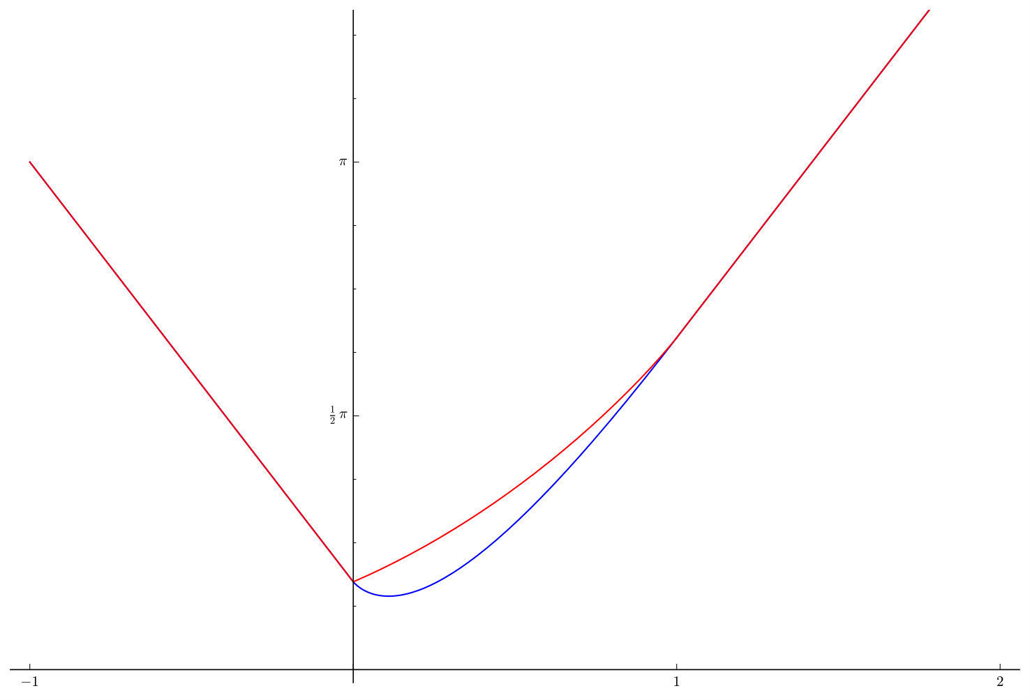 Figure 1
Peer Reviews
No public reviews on file for this paper yet. If you reviewed it on a platform where reviews are public (OpenReview, ICLR, NeurIPS, ICML), you can paste yours below so the community can read it here.
Videos
No videos yet. Explain this paper in a talk, walkthrough, or lecture? Add one.
Intrinsic and dual volume deviations of convex bodies and polytopes
Florian Besau, Steven Hoehner and Gil Kur
Abstract
We establish estimates for the asymptotic best approximation of the Euclidean unit ball by polytopes under a notion of distance induced by the intrinsic volumes. We also introduce a notion of distance between convex bodies that is induced by the Wills functional, and apply it to derive asymptotically sharp bounds for approximating the ball in high dimensions. Remarkably, it turns out that there is a polytope which is almost optimal with respect to all intrinsic volumes simultaneously, up to absolute constants.
Finally, we establish asymptotic formulas for the best approximation of smooth convex bodies by polytopes with respect to a distance induced by dual volumes, which originate from Lutwak’s dual Brunn–Minkowski theory.
††2010 Mathematics Subject Classification: 52A20, 52A27 (52A22, 52A39, 52B05, 52B11)††Key words and phrases: polytopal approximation, intrinsic volume, quermassintegral, dual volume, Wills functional
1 Introduction
The approximation of convex bodies by polytopes is a classical topic in geometry with an extensive history; we refer the interested reader to, e.g., the surveys [3, 21, 51] and the monograph [45] for a proper treatment of the subject.
In this article, we focus on the asymptotic best approximation of the Euclidean unit ball . A natural question dating back to Fejes Tóth [29, Ch. 5.5] is: How well can we approximate the volume of the Euclidean unit ball by an inscribed polytope with vertices? Gruber [41, 42] answered this question asymptotically not only for the ball, but for all smooth convex bodies in all dimensions (see also [9] for generalizations to less smooth bodies and [36, 37] for constructions). For example, if we fix and consider the set of all polytopes that are contained in and have at most vertices, then Gruber’s result, together with asymptotic results for the dimensional constants obtained by Gordon, Reisner and Schütt [38] and improved by Mankiewicz and Schütt [65, 66], imply
[TABLE]
Here and throughout the paper, denotes the -dimensional volume of a compact set in , and we use the asymptotic notation to indicate that the sequence grows at most at the rate does, i.e., . The exact value of the dimensional constant on the right-hand side of (1) is only known for . Results similar to (1) have been obtained for the mean width and volume functionals with a positive continuous weight function [35, 55]. More recently, results of a similar nature were obtained for convex bodies in spaces of constant curvature, such as, for example, the unit sphere [7, 31]. In addition, results on volume best approximation have recently found applications in statistical machine learning theory [24, 25, 26, 27, 53].
Remarkably, as noted by Schütt and Werner [76, Sec. 1.5], when comparing (1) with the expected volume difference of a random polytope generated as the convex hull of independent random points chosen uniformly from the unit sphere , one finds
[TABLE]
(see also [1, 23, 69] and Theorem 13 below). Observe that the difference between the dimensional constants in the right-hand sides of (1) and (2) is of the order and therefore vanishes as . Moreover, the dimensional constant in (1) is bounded above by the dimensional constant in (2), which can be calculated explicitly for all (see (43) below). If one replaces volume by surface area or mean width, then similar observations can be drawn by comparing results on best approximation [12, 18, 49, 55, 57, 73] and on random approximation [4, 5, 13, 17, 20, 71, 72, 76, 79, 80].
In this paper, we are interested in comparing the random and best approximation of the Euclidean unit ball with respect to the intrinsic volumes, which are also known as quermassintegrals. More precisely, the intrinsic volumes for are implicitly defined for any convex body via Steiner’s formula
[TABLE]
More explicitly, by Kubota’s integral formula, we have that
[TABLE]
where is the Grassmannian of all -dimensional linear subspaces of , is the uniquely determined Haar probability measure on , and denotes the orthogonal projection of to . Note that the th intrinsic volume is just the volume, the th intrinsic volume is half of the surface area, and the first intrinsic volume is the same as the mean width, up to a dimensional constant (see Section 3 for more background). By Hadwiger’s theorem, the intrinsic volumes span the space of all continuous rigid motion invariant valuations, and they are normalized such that if is -dimensional, then is exactly the -dimensional Lebesgue measure of .
To measure the distance between two arbitrarily positioned convex bodies and , we introduce the th intrinsic volume deviation by setting
[TABLE]
By Groemer’s extension theorem (see, e.g. [74, Thm. 6.2.5]), the th intrinsic volume can be extended to a valuation on the lattice generated by all finite unions of convex bodies, also denoted by . Then and we can write
[TABLE]
The th intrinsic volume deviation is symmetric, nonnegative and definite, i.e., if and only if . However, is not a metric for , as in general it does not satisfy the triangle inequality (see Appendix A). It is continuous on the metric space of convex bodies in that contain the origin in their interiors, equipped with the Hausdorff distance. Note that is the symmetric difference metric (or Nikodým distance) and is half of the symmetric surface area deviation; see, e.g., [30]. Furthermore, is related to the metric considered in [35, 55], and in Appendix C we compare these two notions of distance.
Finally, in the dual Brunn–Minkowski theory introduced by Lutwak [58], we can make sense of all of the above constructions by essentially replacing the intrinsic volumes with the dual volumes . This leads to the notion of dual volume deviations, for which we are able to establish best and random approximation estimates for general convex bodies.
Organization of the paper
In the next section, we state our main results. In Section 3, we collect important preliminary results before proving our main theorems in Sections 4–6. In the final section, Section 7, we consider stochastic extensions of the Wills and dual Wills functionals. We also include an Appendix with Sections A–C where we prove results that we believe are well-known but could not find suitable literature, and also provide estimates for the hidden constants in most of our statements.
2 Statement of principal results
For a fixed convex body , , we are interested in minimizing the functional , , where special restrictions are imposed on the convex polytopes . We therefore set
[TABLE]
where is a fixed subset of the class of all convex polytopes in . We focus on the following classical types of polytopes:
[TABLE]
In case of the ball, that is, , we simply write , and . For each of these classes , it follows from a compactness argument that there exists a best-approximating polytope of that achieves the minimum in (5).
2.1 Intrinsic volume approximation of the Euclidean ball
Theorem 1**.**
Fix and let . Then there exist absolute constants such that for all sufficiently large , the following inequalities hold true:
- i)
for the inscribed case or the circumscribed case ,
[TABLE] 2. ii)
in the case ,
[TABLE] 3. iii)
in the general position case ,
[TABLE] 4. iv)
and in the general position case ,
[TABLE]
for some absolute constant ; see Remark 2.3.
We prove Theorem 1 in Section 4. Not all results stated in this theorem are new. For more specific information on the known special cases of Theorem 1, please see the discussion in Subsection 2.5 below.
Remark 2.1**.**
In the proof of Theorem 1 i) for or , we derive the asymptotic inequalities
[TABLE]
Here denotes the surface area of , and and are positive constants that depend only on the dimension. These constants appear in the volume and mean width best approximations, see [42] and [35], respectively, as well as Subsection 3.2. In particular, (6) implies
[TABLE]
It is known that [65, 66] and [48]. Thus, the absolute constants in Theorem 1 are asymptotically
[TABLE]
Unfortunately, (6) does not imply the existence of the limit . To the best of our knowledge, the limit is only known to exist for and , and the other cases remain open.
Remark 2.2**.**
The case and poses a notable exception because
[TABLE]
This follows from the fact that the volume of the cone generated by the origin and a facet tangent to the ball is exactly times the volume of the facet. This does not apply for general convex bodies, and in [12] a limit theorem was established for the surface area best approximation of convex bodies by circumscribed polytopes with a bounded number of facets.
Remark 2.3**.**
Note that in Theorem 1 iii), the upper bound is better for lower order than the upper bound . On the other hand, for higher order , e.g., for some , the upper bound is better than . From [53, Thm. 2.4] and the proof of Theorem 1 iv) for , it follows that iv) holds for provided . Moreover, by [53, Rmk. 2.6] and the proof of iv), the bound on the number of facets can be improved to , which causes a change to the value of . For , the value of was given in [53, Rmk. 2.5] in the cases and (see Theorem 18 and Remark 4.1 below). Using these values, can be estimated recursively for using the argument in the proof of iv). Please see Subsection 4.4 for more details.
2.2 Polytopes with a bounded number of -faces
Instead of bounding the number of vertices or facets of the approximating polytopes, one may ask for results on best approximation with respect to polytopes that have a bounded number of -faces. In this setting, asymptotic bounds for the volume and mean width were previously obtained in [10]. More recently, asymptotic results were obtained for the volume [15] and Hausdorff [14] approximations of convex bodies in by polytopes with a restricted number of edges.
For a polytope in and an integer , let denote the number of -faces of . For all and any polytope , by the handshaking lemma we have
[TABLE]
For a simplicial polytope , these inequalities can be extended to
[TABLE]
where denotes the integer part of . This result is due to Björner [8], who called this property of the -vector of a simplicial polytope in its “75% unimodality”.
Using (9) and (10), we derive an immediate corollary to Theorem 1. Define the following classes of polytopes in :
[TABLE]
We also let and denote the corresponding subsets of simplicial polytopes. Note that and .
Corollary 2**.**
Let and .
- i)
For inscribed polytopes with a bounded number of edges, that is, , or for circumscribed polytopes with a bounded number of ridges, that is, , it holds that
[TABLE]
- ii)
Fix . Then
[TABLE]
- iii)
Fix . Then
[TABLE]
Proof.
By (9) we have . Thus, by Theorem 1 i) and (6) we obtain
[TABLE]
The case and parts ii) and iii) follow analogously by (9) and (10). ∎
Equivalently, we may formulate Corollary 2 as a bound on the minimal number of -faces of an inscribed or circumscribed simplicial polytope required to obtain an -approximation of the ball with respect to the intrinsic volume deviation.
Corollary 3**.**
Let and . There exist absolute constants , such that the following holds true for all sufficiently small :
- i)
If is a simplicial polytope such that , then
[TABLE]
for all . For , this bound holds true even if is not simplicial. 2. ii)
If is a simplicial polytope such that , then
[TABLE]
for all . For , this bound holds true even if is not simplicial.
Proof.
Let be a simplicial polytope such that . Set . If is sufficiently small, then has to be large. Thus, by (12) we find
[TABLE]
Since , there exists an absolute constant such that for all . Therefore,
[TABLE]
which establishes i). With similar arguments, ii) follows. ∎
Remark 2.4**.**
One may also consider simple polytopes instead of simplicial polytopes and derive corresponding results. Since the polar of a simple polytope is simplicial, the -vector of simple polytope is also “75% unimodal”, i.e.,
[TABLE]
2.3 Simultaneous approximation and the Wills deviation
From the proof of Theorem 1 follows a remarkable approximation property of the Euclidean ball: There is a polytope which is almost optimal for the ball with respect to all intrinsic volumes simultaneously.
Corollary 4**.**
For all sufficiently large there exist polytopes , respectively , such that
[TABLE]
where are the same absolute constants from Theorem 1.
For another way to quantify how well a polytope approximates the ball in all intrinsic volumes simultaneously, we shall use the classical Wills functional (see, e.g., [68, 81]). For convex bodies , we therefore define the Wills deviation by
[TABLE]
The Wills deviation is continuous on convex bodies that contain the origin in their interiors and is positive definite, but in general it does not satisfy the triangle inequality; see Appendix A for specific counterexamples.
Theorem 5**.**
Set . Then with the same absolute constants from Theorem 1 and another absolute constant , for all sufficiently large the following estimates hold true:
[TABLE]
Furthermore, the bound in ii) for and the bound in iii) for also hold true for nonsimplicial polytopes.
We prove Theorem 5 in Section 5. In Section 7 we consider a generalization of Theorem 5 (see Theorem 22) for the stochastic Wills functional, which is an extension of the Wills functional introduced by Vitale [81]. This extension can also be found in [46] without the probabilistic notation (see also [52]).
Remark 2.5**.**
Since (see (3)), we can express as
[TABLE]
Note that and W(D_{n})\leq\exp(V_{1}(D_{n}))=O\big{(}\exp(\sqrt{n})\big{)} (see, e.g., [68]).
We say that a convex body admits a rolling ball (from the inside) if at every boundary point of there exists a Euclidean ball contained in of positive radius that touches at . As a corollary of results in [13, 71], we extend the upper bound in Theorem 5 i) from the ball to all convex bodies with a rolling ball. This result is proven in Section 5.
Theorem 6**.**
Let be a convex body that admits a rolling ball from the inside. Then
[TABLE]
where is defined by (46) for , is the th normalized elementary symmetric function of the (generalized) principal curvatures of at , and is the surface area measure of , i.e., the -dimensional Hausdorff measure in restricted to .
If , then the right-hand side of (14) is asymptotically equal to , and therefore is asymptotically equal to the upper bound obtained in Theorem 5 i). Since , inequality (14) also gives a trivial asymptotic upper bound for the Wills deviation of and an arbitrarily positioned polytope with at most vertices.
2.4 Dual volume approximation of convex bodies
The classical Brunn–Minkowski theory arises from the combination of volume and the Minkowski addition of convex bodies. The dual Brunn–Minkowski theory, introduced by Lutwak [58, 60, 61], originates by replacing Minkowski addition with radial addition. Many classical notions from the Brunn–Minkowski theory, such as the Brunn–Minkowski inequality, mixed volumes, surface area and curvature measures, etc., have found “dual” analogues in this theory. We refer to [2, 6, 16, 19, 50, 63, 82] for the most recent progress, and to [33, 34] for a succinct introduction.
The radial addition of two convex bodies and that contain the origin in their interiors is defined by
[TABLE]
The set is a star body, but in general it is not convex. Radial addition gives rise to the radial (or dual) Steiner formula
[TABLE]
which implicitly defines the dual volumes . For other recent generalizations of Steiner’s formula, see [70, 78]. Here we have used the normalization for , which is different from the one considered in [34]. More explicitly, Lutwak [59] established the following “dual” to Kubota’s formula (3):
[TABLE]
The dual volumes are continuous, rotation-invariant valuations on convex bodies that contain the origin in their interiors.
We are interested in approximating the dual volume of a convex body by polytopes. Hence, we define the th dual volume deviation between two convex bodies and that contain the origin in their interiors as
[TABLE]
Please note that a notion of dual volume difference was previously considered in [64].
To state our next theorem, we need some more notation. Define the weighted curvature measure of a convex body in that contains the origin in its interior by
[TABLE]
Here is the surface area measure on the boundary of , i.e., the -dimensional Hausdorff measure in restricted to , and denotes the generalized Gauss–Kronecker curvature. Notice that is a weighted version of Blaschke’s classical notion of affine surface area , which was extended from smooth convex bodies to all convex bodies by Schütt and Werner [75], and independently by Lutwak [62] (see also [54]). The affine surface area is equi-affine invariant, that is, for all and , whereas is only rotation invariant for , i.e., for all orthogonal transformations . Furthermore, since is upper semi-continuous (see [62] and [56]), it follows that is upper semi-continuous on all convex bodies that contain the origin in their interiors.
Theorem 7**.**
Let be a convex body of class that contains the origin in its interior and let . Furthermore, let be either , , , or , and set
[TABLE]
Then
[TABLE]
Please see Subsection 3.3 for more information on the dimensional constant .
We prove Theorem 7 in Section 6 by relating the problem to the weighted volume best approximation of convex bodies as considered in [35, 55]. In Theorem 21 below, we extend this result from to all by considering the natural analytic extension of the dual volumes from to .
Random approximation of convex bodies with respect to the intrinsic volumes has been considered before in [1, 13, 71]. By an extension [83, Satz 10.1] of the random approximation results in [13] to weighted volumes (see Theorem 16 below), we derive the following random approximation results for the dual volumes.
Theorem 8**.**
Let be a convex body that admits a rolling ball and contains the origin in its interior. Choose points at random from independently and according to the probability density function defined by
[TABLE]
for all where is defined, and set otherwise.
- i)
Set . Then
[TABLE] 2. ii)
Assume further that is of class and set , where is the closed supporting halfspace of at that contains . Then for any convex body that contains in its interior,
[TABLE]
This result follows from Theorem 16, Theorem 17 and Lemma 19. Please see Subsection 6.1 for more details.
Remark 2.6**.**
More generally, a similar limit theorem holds in Theorem 8 for any continuous probability density . However, by Hölder’s inequality it follows that is the optimal density, i.e., the right-hand side of (20) is minimal for (see Subsection 6.1). In particular, we find that
[TABLE]
Thus, also in the dual setting we see that best and random approximation are asymptotically equivalent in high dimensions.
The proof of this remark is given in Appendix B; see (107) and (110).
We also motivate the definition of a dual Wills functional for a convex body that contains the origin in its interior by
[TABLE]
and we define the dual Wills deviation by
[TABLE]
for all convex bodies and that contain the origin in their interiors.
Theorem 9**.**
Let be a convex body of class that contains the origin in its interior. Furthermore, let be either , , , or , and set as in (19). Then
[TABLE]
Moreover, if is a convex body that admits a rolling ball from the inside and contains the origin in its interior, then
[TABLE]
and if is a convex body of class and contains the origin in its interior, then
[TABLE]
We prove Theorem 9 in Subsection 6.1 using an extension of results in [13] for the weighted random approximation of convex bodies. Please see Theorem 16 below for more details.
Remark 2.7**.**
For the inscribed case we have
[TABLE]
and for the circumscribed case we have
[TABLE]
Therefore, the lower and upper bounds in Theorem 9 are almost equal in high dimensions; see (106) and (110) in Appendix B for the details.
2.5 Comparison with known results
To the best of our knowledge, this paper is the first to give estimates for intrinsic volume approximation by arbitrarily positioned polytopes. It is also the first to give asymptotically sharp lower bounds for the best inscribed and circumscribed approximations of the ball. In particular, the inscribed result shows that the random construction of Affentranger [1] is optimal up to a term of order . Thus, as the dimension tends to infinity, random approximation of the ball by inscribed polytopes is as good as best approximation under the intrinsic volume deviation; see Corollary 14. The main results of this paper address questions of Gruber, who asked for estimates on asymptotic best approximation of convex bodies by polytopes with respect to intrinsic volumes ([45], p. 216). Most of the bounds in Theorem 1 were previously known only for . More specifically:
For and , one may use the Steiner formula and results on approximation of convex bodies under the Hausdorff distance [73] to obtain an upper bound for general convex bodies; see [35]. In particular, by this argument one may obtain the upper bound in Theorem 1 i). The upper bound for and also follows from [1, Thm. 5]. 2. 2.
For and , the limit theorems in [9, 43, 55] for the symmetric volume difference of convex bodies of class , together with estimates for the dimensional constants in [10, 48, 53, 57, 65, 66], imply precise bounds for the ball. 3. 3.
For and , the upper bound in Theorem 1 ii) was established in [36]. 4. 4.
For and , an upper bound for convex bodies of class was recently established in [39]. Previously, an upper bound for and was given in [49] for the special case of the ball. 5. 5.
For and , a lower bound was established in [49] and an upper bound was established in [53]. 6. 6.
For , the intrinsic volume deviation is related to the metric defined by
[TABLE]
where is the unit sphere, is the uniform probability measure on and is the support function of . We have with equality if and only if is convex; see Theorem 25 in Appendix C. Hence, for , the limit theorems in [9, 35] for the approximation of convex bodies by polytopes under , together with the estimates for the dimensional constants in [48, 53, 65, 66], yield precise bounds also for .
However, for one only has in general, and therefore we have to distinguish between the two notions. For , limit theorems were obtained by Ludwig [55] and estimates for the dimensional constants can be found in [53, 57]. By a result of Eggleston [28], it follows that in the plane we have , i.e., a polygon with vertices is best-approximating for the unit disk if and only if it is inscribed. In particular, this yields for all . Very recently, Fodor [31] proved an analogue of Eggleston’s result for the hyperbolic plane , and showed that it fails on the sphere .
To the best of our knowledge, polytopal approximation of convex bodies with respect to the Wills functional and stochastic Wills functional have not been considered before, and our asymptotic bounds in the inscribed and circumscribed cases are optimal, up to absolute constants. Furthermore, approximation with respect to dual volumes also appears to be new and, as we show, is strongly tied to best and random approximation of convex bodies with respect to weighted volumes as considered in [13, 35, 55, 71, 76].
3 Preliminaries
As a general reference on convex bodies, we refer to the monographs [32, 45, 74]. In the following, we collect the necessary notions and classical results on best and random approximation needed in our proofs.
Notation and Definitions
We shall work in -dimensional Euclidean space , , equipped with inner product and Euclidean norm . For , we set .
A convex body is a convex and compact subset of with nonempty interior. We write for the space of convex bodies in endowed with the Hausdorff metric, and denotes the subspace of convex bodies in that contain the origin in their interiors. The boundary of a convex body is denoted , and denotes the surface area measure of . The -dimensional volume of is , and its surface area is denoted .
The Euclidean unit ball is the set . Its boundary is the unit sphere , and denotes the uniform probability measure on , i.e., . The volume of the Euclidean unit ball is , and . The following asymptotic estimate is used frequently (see Appendix B (98)):
[TABLE]
The support function of is defined by , where . The polar body of is defined by .
3.1 Background on intrinsic volumes
The intrinsic volumes of a convex body are completely determined by Steiner’s formula (see, e.g., [74, Eqn. (4.1)])
[TABLE]
Note that is the set of all points with distance at most from , i.e., where . In particular, .
The intrinsic volumes are monotonic, i.e., if then . Thus, for all . The first intrinsic volume of is called the intrinsic width of , and Kubota’s integral formula (3) yields
[TABLE]
The famous Alexandrov–Fenchel inequalities for mixed volumes imply the following well-known inequalities.
Theorem 10** (Isoperimetric inequalities for intrinsic volumes).**
Let .
- i)
Extended isoperimetric inequality: For any ,
[TABLE]
Equality holds for any one of the inequalities, and then throughout all of them, if and only if is a Euclidean ball, i.e., for some and . 2. ii)
The sequence is log-concave, i.e., for all ,
[TABLE]
Equality holds in (34) if for some and , but there is no complete characterization of the equality cases of (34). For more background on the Alexandrov–Fenchel inequalities and their numerous consequences, see, e.g., [74, Ch. 7].
In (33) and (34) one may replace the intrinsic volume with some other renormalization. In particular, the classical isoperimetric and Urysohn inequalities are special cases of (33):
[TABLE]
3.2 Best approximation of convex bodies by polytopes
First, let us briefly remark on the well-posedness of our best-approximation problems. By the definition of , we have , where denotes a fixed class of polytopes from . Since polytopes are dense in the space of all convex bodies with respect to the Hausdorff metric and since is positive definite, we conclude that monotonically decreases to [math] as . In particular, this implies that there are sequences such that , and as .
To prove the existence of minimizers in , one may argue as follows. Let and let be arbitrary. The support function of a convex polytope is
[TABLE]
The mapping is continuous with respect to the -norm on continuous functions on , and therefore the mapping is continuous with respect to the Hausdorff metric. Hence, if we draw points from a convex compact subset , then the continuity of the functional yields the existence of a best-approximating polytope such that . More generally, one can show that if contains a closed ball of radius in its interior and is contained in an open ball of radius , i.e., and for some , and if is small, then necessarily . Hence, again by compactness and continuity, if is large enough there exists a best-approximating polytope such that for .
In the proof of Theorem 1, we apply a result of Gruber [44] for the Euclidean unit ball. Fejes Tóth [29] stated a version of this theorem in the plane, which was later proven by McClure and Vitale [67].
Theorem 11** ([44, Thm. 1]).**
Fix and let be a convex body of class . Then
[TABLE]
where is the affine surface area of defined in (18).
Gruber proved this theorem for convex bodies of class (i.e., convex bodies with everywhere positive Gauss–Kronecker curvature), which was subsequently weakened to by Böröczky [9]. Observe that asymptotically, the best approximation is determined by the affine surface area of and the constants and which depend only on the dimension . We briefly recall estimates for these constants in the next section. For the ball, we have and therefore
[TABLE]
Glasauer and Gruber [35] obtained similar limit theorems for convex bodies of class and the metric . We only state their results for the unit ball.
Theorem 12** (Corollary to [35, Thm. 1]).**
The following asymptotic formulas hold true:
[TABLE]
Remark 3.1**.**
Please note that Glasauer and Gruber actually state Theorem 12 in terms of the -metric . In the case of inscribed and circumscribed polytopes, and agree, up to a dimensional constant. In general, with equality if and only if is convex. For more information, see Appendix C.
3.3 Delone triangulation and Dirichlet–Voronoi tiling numbers
The constants and are called the Delone triangulation and Dirichlet–Voronoi tiling numbers in , respectively. They were introduced by Gruber in [44] and are named after Delone triangulations and Dirichlet–Voronoi tilings in , which are dual tessellations of that arise in the proofs of the asymptotic formulas (35) and (36) in [44]. The exact values of these constants are known explicitly only for and . Fejes Tóth [29] derived the values and . The values and were later determined by Gruber in [41] and [42], respectively. For , the exact values of and are unknown, but their asymptotic behavior has been estimated quite precisely. The best-known asymptotic estimates for and are:
[TABLE]
The estimate for is due to Mankiewicz and Schütt [65, 66], and the estimate for is due to Hoehner and Kur [48].
Laguerre–Delone triangulation and Laguerre–Dirichlet–Voronoi tiling numbers.
The dimensional constants and that appear in Theorem 7 are called the Laguerre–Delone and Laguerre–Dirichlet–Voronoi tiling numbers in , respectively. They were introduced by Ludwig [55] and are connected with Laguerre–Delone and Laguerre–Dirichlet–Voronoi tilings in , respectively. These tilings arise in the proofs of the asymptotic formulas (82) for arbitrarily positioned polytopes in [55]. For , it is known that (see, e.g., [55]). For , Gruber [41] conjectured that . Böröczky and Ludwig [18] later proved that this is the correct value, and they also established that . For , the exact values of and are again unknown. It has been determined that there exist positive absolute constants such that
[TABLE]
The lower and upper estimates for are due to Böröczky [10] and Ludwig, Schütt and Werner [57], respectively, and the lower and upper estimates for are due to Ludwig, Schütt and Werner [57] and Kur [53], respectively. In fact, Kur [53] gave the estimates
[TABLE]
Closing the dimensional gap between the upper and lower estimates for appears to be a difficult open problem.
3.4 Intrinsic volume approximation of convex bodies by random polytopes
Random constructions have frequently been used to generate well-approximating polytopes. Remarkably, it turns out that in many cases, as the dimension tends to infinity, random approximation of smooth convex bodies is asymptotically as good as best approximation. This phenomenon has been observed in, e.g., the volume approximation by inscribed polytopes [43, 76]; volume, surface area, and mean width approximation by circumscribed polytopes [11, 12, 35, 43]; and volume [48, 53, 57] and surface area [49, 53] approximation by arbitrarily positioned polytopes.
Affentranger [1] proved the following asymptotic formula for the approximation of the ball by inscribed random polytopes under the intrinsic volume difference.
Theorem 13** ([1, Thm. 5]).**
Choose points independently with respect to the uniform probability measure on the unit sphere , and set . Then
[TABLE]
where
[TABLE]
In Appendix B we verify that for all ,
[TABLE]
Thus, the constant from Theorem 1 i) for agrees with the constant in the right-hand side of (42), up to an error term of order . This is summarized in the following corollary, where our estimates can be found in Appendix B.
Corollary 14**.**
Choose points independently with respect to the uniform probability measure on the unit sphere , and let . Then for every ,
[TABLE]
More generally, Reitzner [71] obtained an asymptotic formula for the expected th intrinsic volume difference for convex bodies, which was extended in [13] to convex bodies that admit a rolling ball from the inside.
Theorem 15** ([71, Thm. 1] and [13, Thm. 1.2]).**
Let be a convex body that admits a rolling ball from the inside. Choose points at random from independently according to a positive, continuous probability density function , and let . Then
[TABLE]
where is a positive constant that depends only on and , and for , is the th normalized elementary symmetric function of the (generalized) principal curvatures of at .
Putting and comparing (45) with (42) yields
[TABLE]
and in particular,
[TABLE]
Using Hölder’s inequality, Reitzner showed that the right-hand side of (45) is minimized by the probability density
[TABLE]
Choosing this density in (45) yields
[TABLE]
Let be a continuous function. As a generalization of the volume difference, one defines the -weighted volume difference by
[TABLE]
Best approximation with respect to the -weighted volume difference was considered in [55] (see Theorem 20 below). We need the following generalization of the random approximation for the volume difference to the weighted volume difference, which was obtained in [83]. This result is an extension of [13, Thm. 1.1] for the case (see also [76]).
Theorem 16** ([83, Satz 10.1], weighted volume extension of [13, Thm. 1.1]).**
Let be a convex body that admits a rolling ball from the inside, and let be a weight function on that is continuous near the boundary of and such that . Choose points at random from independently according to a continuous probability density function , and let . Then
[TABLE]
Using Hölder’s inequality, we derive that given , the minimal value of the right-hand side of (50) is achieved for the probability density
[TABLE]
Choosing this density in (50) yields
[TABLE]
A dual random construction that generates random polytopes which are circumscribed around a convex body was considered in [20]. Choose points randomly and independently from the boundary of a convex body of class , and consider the random polyhedral set that is the intersection of all the closed halfspaces of , where is the uniquely determined supporting halfspace of at .
Theorem 17** ([20, Thm. 1]).**
Let be a convex body of class and let be an arbitrary convex body that contains in its interior. Choose points at random from independently according to a continuous probability density function , and set . If is a continuous and bounded weight function, then
[TABLE]
The optimal density is given by as defined in (51), and in this case
[TABLE]
Note that results for and were also obtained in [20].
Remark 3.2**.**
The curvature conditions on in Theorem 17 were recently weakened in [83, Satz 10.4], where one only requires that slides freely inside a ball, which is equivalent to the property that admits a rolling ball from the inside (where we may assume without loss of generality that contains the origin in its interior). However, since in this case may have singular points, i.e., there might be more than one support hyperplane at a fixed boundary point, one has to consider a probability distribution on the set of all hyperplanes that envelop the convex body instead of a probability distribution on .
In fact, as was observed in [83], the random polytope is in distribution equivalent to the polar of a random polytope with vertices chosen at random from the boundary of with respect to a distribution determined by the distribution of the halfspaces that generate .
4 Intrinsic volume approximation of the ball
In this section we prove Theorem 1.
4.1 Proof of Theorem 1 i): Inscribed and circumscribed case
Let . By Theorem 10 i),
[TABLE]
Taking the minimum over all in we obtain
[TABLE]
Thus, using Theorem 11 and Theorem 12, as well as the formulas for and , we derive that
[TABLE]
Analogously, if then
[TABLE]
Now taking the minimum over all in we deduce
[TABLE]
Hence, again by Theorem 11 and Theorem 12 we conclude
[TABLE]
∎
4.2 Proof of Theorem 1 ii): Inscribed case with bounded number of facets
As remarked in [36], it was proved in [22] that there is an absolute constant such that for all sufficiently large , there exists a polytope such that
[TABLE]
Thus, by Theorem 10 i), for any and all sufficiently large it holds true that
[TABLE]
Hence, for all sufficiently large ,
[TABLE]
and therefore
[TABLE]
This proves Theorem 1 ii). ∎
4.3 Proof of Theorem 1 iii): General position and bounded number of vertices
Let be a random polytope generated by random vertices chosen independently and uniformly from . Set
[TABLE]
so that and . In the proof of [57, Thm. 1] (more specifically, [57, Eq. (9) and (28)]), it was shown that there exists an absolute constant such that for all sufficiently large ,
[TABLE]
where is determined by
[TABLE]
(See [57, Eq. (10)] and [40, Eq. (3.14)] for similar results.) Hence , and since as we derive that
[TABLE]
for some absolute constant when is large enough. We aim to show that there exists an absolute constant such that
[TABLE]
which will yield the desired upper bound since .
Let be arbitrary. By the aforementioned result of Affentranger in Theorem 13, there exists such that for all ,
[TABLE]
This yields
[TABLE]
Similarly, we obtain
[TABLE]
We have and
[TABLE]
which is proven in Appendix B. Since was chosen arbitrarily, this yields
[TABLE]
and . Thus, there exists such that for all
[TABLE]
Since , we deduce that
[TABLE]
which yields
[TABLE]
by monotonicity. Moreover,
[TABLE]
for some absolute constants and all sufficiently large . Thus, when is large enough,
[TABLE]
Since , this yields that for all ,
[TABLE]
where for . By Theorem 10 i) we derive
[TABLE]
To continue, we would like to apply a Bernoulli-type inequality, but to do so we need to verify that
[TABLE]
holds true with high probability if is large. Consider the event . If and if , then
[TABLE]
Since as , this shows that (67) holds true for the event for sufficiently large . Furthermore, using Chebyshev’s inequality, a variance bound obtained by Reitzner [72, Thm. 8] and Theorem 13 for , we bound the probability of the complementary event by
[TABLE]
for some positive constant that only depends on the dimension . The trivial upper bound
[TABLE]
and together yield
[TABLE]
Next, we apply the Bernoulli-type inequality for and to derive that under the event , for all sufficiently large any realization of the random variable satisfies
[TABLE]
Therefore, by the previous two inequalities, as well as (63), (66) and (68), we finally obtain that for large enough ,
[TABLE]
Thus, (64) holds true. ∎
4.4 Proof of Theorem 1 iv): General position and bounded number of facets
We shall show that there is an absolute constant and an absolute constant such that for all sufficiently large , there exists a polytope such that
[TABLE]
We will use a recursive argument to prove (69). The main idea is to use Theorem 10 ii) and bounds on and to derive an upper bound on , iterating from to . More specifically, we show that in the th step of the recursion, for some absolute constant . The hypothesis is necessary because the constants blow up fast. To prove the existence of the polytope , we use the following result of Kur [53] to initialize the recursion.
Theorem 18** (Remark 2.5 in [53]).**
There exists an absolute constant such that for every and there exists a polytope in with at most facets which satisfies both of the following inequalities simultaneously:
[TABLE]
Remark 4.1**.**
It was shown in [53] that
[TABLE]
where is the exponential integral and is the Euler–Mascheroni constant. It was also shown in [53] that the inequalities (70) hold simultaneously provided , but with a different constant .
Proof of Theorem 1 iv)
We argue by induction on to show that for all , the polytope from Theorem 18 satisfies
[TABLE]
Since , this only improves the upper bound for if is so small that . Hence in the upper bound in Theorem 1 iv), we restrict for some absolute constant .
The statement (71) is true for by Theorem 18. So let , and we will show that the statement (71) holds true for . Inequality (70) implies that for all ,
[TABLE]
Hence, for all ,
[TABLE]
By Theorem 10 i), (72) and Bernoulli’s inequality we obtain
[TABLE]
for all . Analogously, by (73) we derive
[TABLE]
for all . The monotonicity of and the induction hypothesis (71) imply
[TABLE]
for all large enough. Moreover, by Theorem 10 ii) we have
[TABLE]
for all . Finally, by (74) and (4.4) we derive
[TABLE]
for all . Hence (71) holds true for . ∎
5 Simultaneous approximation and the Wills functional
In this section we prove Corollary 4, Theorem 5 and Theorem 6.
5.1 Proof of Corollary 4: Simultaneous approximation of the Euclidean ball
By (55), we derive that for any polytope ,
[TABLE]
Taking the minimum over and the limit as , we conclude
[TABLE]
Hence the corollary follows for the case . Analogously, we derive the case from (58). ∎
5.2 Proof of Theorem 5: Bounds for the Wills deviation for the Euclidean ball
Proof of i).
The lower bound follows directly from Theorem 1 i) and (6) since
[TABLE]
For the upper bound, we only prove the case as the case follows similarly by performing the obvious modifications. Let be arbitrary. By Theorem 11, there exists such that for all there exists that satisfies
[TABLE]
Then by Theorem 10 i), for all we have
[TABLE]
This implies that for all ,
[TABLE]
Since was arbitrary, the result follows. ∎
Proof of ii) and iii).
Analogously to i), Theorem 5 ii) and iii) follow from Corollary 2.∎
Proof of iv).
Analogously to i), Theorem 5 iv) follows from summing inequality (61) over . ∎
Proof of v).
In the proof of Theorem 1 iii), specifically (64), it was shown that when is sufficiently large, the random polytope satisfies
[TABLE]
where . Recall that holds with probability . Notice that by Theorem 13 we have
[TABLE]
By (100) in Appendix B, is strictly increasing in , so if is large enough then
[TABLE]
Furthermore, by (103) in Appendix B we derive
[TABLE]
for some absolute constant . Hence,
[TABLE]
which yields
[TABLE]
Thus, if is sufficiently large, then for all we have
[TABLE]
with high probability for some absolute constant . Hence, if is sufficiently large, then with high probability
[TABLE]
Since this holds true with positive probability, if is large enough there exists a realization of which verifies the upper bound in Theorem 5 v). ∎
5.3 Proof of Theorem 6: An upper bound for the Wills deviation for convex bodies
Let be a convex body in that admits a rolling ball from the inside. For each , choose points at random from independently and according to the optimal density defined in (47), and let . Using Theorem 15 as in (48), we derive that for each ,
[TABLE]
Now consider the random polytope defined by
[TABLE]
Note that has at most vertices. Thus, since for all , from (77) we obtain
[TABLE]
From this bound on the expectation, it follows that there exists a realization of the random polytope that also satisfies the bound. This concludes the proof.∎
6 Dual volume approximation of convex bodies
For , the radial function is defined by . Integrating with respect to polar coordinates, from (15) we derive that
[TABLE]
Since , we define the analytic extension
[TABLE]
and set
[TABLE]
The quantity is finite since the origin lies in the interior of , and therefore for all . For and , we define the th dual volume deviation by
[TABLE]
For , we set
[TABLE]
and define
[TABLE]
We will need the following lemma, which is related to [34, Thm. 4.1].
Lemma 19**.**
Let .
- i)
If , then
[TABLE] 2. ii)
If , then
[TABLE] 3. iii)
If , then
[TABLE]
Proof.
First, let . Since the origin is an interior point of and , for all we have
[TABLE]
Also, by the elementary fact that for any
[TABLE]
we conclude
[TABLE]
Using polar coordinates and the fact that
[TABLE]
we derive
[TABLE]
The cases and follow from similar arguments. ∎
Remark 6.1**.**
Let . Then . Furthermore, since we have
[TABLE]
with equality if and only if (see Appendix C). A similar observation was also made in [35, Rmk. 3].
For , we use (81) and derive that
[TABLE]
Recall that for a continuous function , the -weighted volume difference is defined by
[TABLE]
By Lemma 19, we can identify approximation in the th dual volume deviation with approximation under the -weighted volume difference. The following results on weighted volume approximation were obtained by Ludwig [55] for convex bodies of class and extended to by Böröczky [9]. Note that Ludwig’s proof for and also gives the corresponding results for the inscribed case (see [43]) and the circumscribed case (see [35]), where only the dimensional constants in the limit need to be changed.
Theorem 20** ([55]).**
Let be a convex body of class . Furthermore, let be either , , , or , and set as in (19). If is a continuous function, then
[TABLE]
We are now ready to prove the following extension of Theorem 7.
Theorem 21**.**
Let be a convex body of class that contains the origin in its interior, let be either , , , or , and set as in (19). For , set
[TABLE]
- i)
If , then
[TABLE] 2. ii)
If , then
[TABLE] 3. iii)
If , then
[TABLE]
Proof.
Let . We would like to use the weight function , which is discontinuous at the origin if . We remedy this by the following standard arguments. Let . Then there exists such that for all , the ball is also contained in the interior of . We define the continuous weight function by
[TABLE]
Notice that for all and . Thus,
[TABLE]
where we extended the definition (18) of to . By Lemma 19, if is a polytope that contains then
[TABLE]
Observe that if is large enough, then any polytope that is well-approximating contains . To see this, for define the closed halfspace and set
[TABLE]
If does not contain , then there exists such that . In this case,
[TABLE]
Since
[TABLE]
we also find that . Furthermore, since and as , there exists such that for all we have and . Thus, if then
[TABLE]
Therefore, by Theorem 20 we have
[TABLE]
which concludes the proof for all . The case follows analogously, and the case follows from (81). ∎
6.1 The dual Wills functional and dual Wills deviation
For , the Wills functional can be expressed as
[TABLE]
where (see, e.g., [81]). For and , the minimal radial distance of to is defined as the minimal distance between and a point such that and the origin are collinear, or equivalently,
[TABLE]
Note that
[TABLE]
Hence, by the radial Steiner formula (15) it follows that
[TABLE]
This motivates us to define the dual Wills functional by
[TABLE]
For , we also define the dual Wills deviation by
[TABLE]
Proof of Theorem 9.
Since
[TABLE]
the lower bound (25) follows from Theorem 7.
For the upper bound, we follow arguments similar to those in Subsection 5.3 using (52). For , we therefore define the continuous, positive and bounded weight function
[TABLE]
where we assume that is so small that is contained in the interior of . Now by Lemma 19 we have
[TABLE]
for all such that . Then the density function corresponding to on that minimizes the right-hand side of (50) and (53) is given by
[TABLE]
see (51). Thus,
[TABLE]
and
[TABLE]
Now we use a random construction similar to the one in Subsection 5.3. For each , choose from independently and according to the density , and set
[TABLE]
Then for all , and therefore
[TABLE]
Similarly, we define by
[TABLE]
where is distributed with respect to for and , and is the supporting halfspace of at . Notice that , and by Theorem 17 we conclude
[TABLE]
Hence, there is a realization of such that
[TABLE]
and similarly there is a realization of such that and
[TABLE]
Therefore, the upper bound (26) holds true. ∎
7 The (dual) stochastic Wills deviation
Vitale [81] generalized the Wills functional (and, in a sense, the Steiner formula) using a probabilistic construction. This construction was also considered by Hadwiger [46] without the probabilistic notation (see also [52, 68]). Consider a random variable on with . Using as the radius in the Steiner formula (31) and taking the expectation, we obtain
[TABLE]
For a nonnegative random variable with finite th moment, we call the -Wills functional, or stochastic Wills functional, which is defined for any convex body . In particular, if is the constant then we recover the Steiner formula (31). Furthermore, if where is a Weibull random variable with parameters , i.e., has the density for , then and we recover the Wills functional of :
[TABLE]
Now, given and a nonnegative random variable with , we define the -Wills deviation by
[TABLE]
Note that the stochastic Wills functional is not a metric in general; a proof is given in Appendix A.
We derive an immediate corollary to Theorem 5.
Corollary 22**.**
Set . Then with the same absolute constants from Theorem 5 and for all sufficiently large , the following estimates hold true:
[TABLE]
Furthermore, the bound in i) for and the bound in ii) for also hold true for nonsimplicial polytopes.
Proof.
In the proof of Theorem 5 i), it was shown that for there exists a polytope which satisfies all of the upper bounds in Theorem 1 i) simultaneously. Thus, for all sufficiently large ,
[TABLE]
so the upper bound in i) holds. Part iv) follows in the same way, but we use Theorem 5 iv) instead. The lower bounds in i), ii) and iii) follow from the lower bounds in Theorem 1 i), ii) and iii), respectively, together with the estimate
[TABLE]
Here the last inequality holds when is large enough, and is the absolute constant from Theorem 1. Finally, v) follows along the same lines as the proof of Theorem 5 v); we leave the details to the interested reader. ∎
Remark 7.1**.**
Similar to Remark 2.5, we notice that
[TABLE]
Remark 7.2**.**
Theorem 6 can be generalized to give an upper bound for the -Wills deviation of a convex body with a rolling ball and an inscribed polytope with a prescribed number of vertices. We leave the details to the interested reader.
7.1 The dual stochastic Wills deviation
For , we define the dual -Wills functional by
[TABLE]
and if as well, we define the dual -Wills deviation by
[TABLE]
As a corollary to Theorem 9, we obtain the following result.
Corollary 23**.**
Let be a convex body of class that contains the origin in its interior. Furthermore, let be either , , , or , and set as in (19). Then
[TABLE]
Moreover, if is a convex body that admits a rolling ball from the inside and contains the origin in its interior, then
[TABLE]
and if is a convex body of class , then
[TABLE]
Furthermore, these upper bounds also hold true for and since and .
Proof.
The corollary follows analogously to Theorem 9, where in the end we just notice that
[TABLE]
Acknowledgments
The authors would like to express their sincerest gratitude to Ferenc Fodor, Daniel Hug, Monika Ludwig, Matthias Reitzner, Christoph Thäle, Viktor Vígh and Elisabeth Werner for the enlightening discussions. The authors would also like to thank the anonymous referees for their valuable comments that helped improve the article. The work of the third author is supported by the Center for Brains, Minds and Machines (CBMM), funded by NSF STC award CCF-1231216.
Appendix A The intrinsic volume deviation and the stochastic Wills functional are not metrics
It is well-known that the symmetric volume difference is a metric on and induces the same topology as the Hausdorff metric on the space of all convex bodies that have nonempty interiors (see, e.g., [77]). On the other hand, the surface area deviation is not a metric since it does not satisfy the triangle inequality. An explicit counterexample was given in [47]. The same triple of convex bodies can be used to show that for any , the th intrinsic volume deviation fails to satisfy the triangle inequality.
Lemma 24**.**
Fix with . For , the intrinsic volume deviation does not satisfy the triangle inequality and is thus not a metric on . Moreover, the stochastic Wills deviation does not satisfy the triangle inequality and is thus not a metric on .
Proof.
Let . We consider the disjoint caps of the ball defined by
[TABLE]
Since and , we have
[TABLE]
Since , we also have . We want to show that , which is equivalent to
[TABLE]
Since the caps converge to half-balls as , by the continuity of the intrinsic volume and its valuation property we obtain
[TABLE]
Thus, since increases monotonically as , there exists such that (92) holds for all . We have thus verified that is not a metric.
Similarly, for the stochastic Wills deviation we want to show that , which holds if and only if
[TABLE]
By (92), for all it holds that
[TABLE]
Therefore,
[TABLE]
Since is a positive random variable, we have . Furthermore, since increases to as , there exists such that
[TABLE]
or equivalently, . Thus, from (94) we obtain , which proves (93). ∎
In this proof we essentially used the discontinuity of the intrinsic volume deviation and of the stochastic Wills functional on . Notice that if is a continuous valuation on , then the deviation functional is continuous on convex bodies that have an interior point in common. However, may not be continuous in general; continuity fails if there are two convergent sequences of convex bodies and such that , and .
Appendix B Asymptotic estimates
Recall that and . By Stirling’s inequality,
[TABLE]
This implies
[TABLE]
and
[TABLE]
Therefore, we also obtain
[TABLE]
which proves (30). We use the local approximation for , which yields
[TABLE]
Estimates for (43) and (46).
We first estimate the constant in (43), which is defined by
[TABLE]
By the formula for , we obtain
[TABLE]
This implies
[TABLE]
and
[TABLE]
Using this estimate as well as (95), (98) and (99), we conclude
[TABLE]
and for all and . Furthermore, by (95) we conclude that for all and ,
[TABLE]
and
[TABLE]
Moreover, we obtain the estimate
[TABLE]
which yields
[TABLE]
For (46), we write and use (98) and (102) to derive the bounds
[TABLE]
Estimates for which yield (22) and (28).
In [66, Thm. 2] it was shown that
[TABLE]
Using (97), (98) and (101), this yields
[TABLE]
and
[TABLE]
Using (104) we conclude
[TABLE]
which yields (28). Now (22) follows similarly from
[TABLE]
Estimates for which yield (39) and Corollary 14.
By [48, Thm. 4], there are absolute constants such that and
[TABLE]
Hence, by (7) and (105) we derive
[TABLE]
where . Thus, to prove Corollary 14 we use (6), (42), (98) and (102) to obtain
[TABLE]
This also yields (29) since
[TABLE]
Appendix C The relationship between and
The intrinsic width is related to the metric (see, e.g. [30]). The intrinsic width also defines the intrinsic width deviation , which is not a metric as we saw in Appendix A.
Theorem 25**.**
Let . Then
[TABLE]
with equality if and only if is convex. In particular, if .
Proof.
Since and , we derive
[TABLE]
We also have that
[TABLE]
Now since , we derive . Therefore,
[TABLE]
with equality if and only if , or equivalently, if and only if . If is convex, then by the valuation property of we have .
We are done once we show that implies that is convex. Assume the opposite. Then for all and there exists a point . Since , there exists such that . Since , we also have . Hence,
[TABLE]
Analogously, there exists such that
[TABLE]
Observe that . If , then , or equivalently,
[TABLE]
Hence and can be strictly separated by a hyperplane with normal direction , that is, , which is a contradiction to .
Thus we may assume that and , i.e., there is a unique minimizing geodesic arc between and on . By the continuity of , there exists on this arc such that . We may write for some . By the subadditivity property of support functions, we conclude
[TABLE]
which is also a contradiction to . Hence is convex. ∎
Remark C.1**.**
If are such that and for some , then by Theorem 25 and , we derive
[TABLE]
In particular, this yields that approximations with respect to and are of the same order.
Example 26**.**
Consider the unit disk in . For let be a regular triangle centered at the origin with circumradius , that is, is inside of if and is inside of if . Thus, since we derive
[TABLE]
For , we calculate that
[TABLE]
See Figure 1 for a plot of the two functions. In particular, the minimum of is achieved for some , i.e., and are in a general position, whereas the minimum of is achieved for , that is, if the regular triangle is inscribed. The latter also follows as a special case of a theorem by Eggleston [28, Lem. 4], who showed that the best-approximating polygon with respect to is always inscribed. Note that in the plane , the first intrinsic volume deviation is the perimeter deviation; see, e.g., [31].
The reference list from the paper itself. Each links out to its DOI / PubMed record.
- 1[1] F. Affentranger, The convex hull of random points with spherically symmetric distributions , Rend. Sem. Mat. Univ. Politec. Torino 49 (1991), 359–383.
- 2[2] D. Alonso-Gutiérrez, M. Henk, and M. A. Hernández Cifre, A characterization of dual quermassintegrals and the roots of dual Steiner polynomials , Adv. Math. 331 (2018), 565–588.
- 3[3] I. Bárány, Random polytopes, convex bodies, and approximation , Lecture Notes in Math. 1892 (2007), Springer, 77–118.
- 4[4] I. Bárány, F. Fodor, and V. Vígh, Intrinsic volumes of inscribed random polytopes in smooth convex bodies , Adv. in Appl. Probab. 42 (2010), 605–619.
- 5[5] I. Bárány and C. Thäle, Intrinsic volumes and Gaussian polytopes: the missing piece of the jigsaw , Doc. Math. 22 (2017), 1323–1335.
- 6[6] A. Bernig, The isoperimetrix in the dual Brunn–Minkowski theory , Adv. Math. 254 (2014), 1–14.
- 7[7] F. Besau, M. Ludwig, and E. M. Werner, Weighted floating bodies and polytopal approximation , Trans. Amer. Math. Soc. 370 (2018), 7129–7148.
- 8[8] A. Björner, Partial unimodality for f 𝑓 f -vectors of simplicial polytopes and spheres , Contemp. Math. 178 (1994), 45–54.