Adaptation and learning over networks under subspace constraints -- Part I: Stability Analysis
Roula Nassif, Stefan Vlaski, Ali H. Sayed

TL;DR
This paper introduces a distributed adaptive algorithm for network optimization under subspace constraints, proving its stability and small estimation errors in the small step-size regime, with further performance analysis in the sequel.
Contribution
It develops a distributed implementation of projected gradient descent for subspace-constrained network optimization, ensuring stability and performance close to centralized solutions.
Findings
Distributed algorithm achieves small estimation errors for small step-sizes.
The proposed method generalizes consensus optimization to broader subspace constraints.
Part II will analyze steady-state performance considering noise and data characteristics.
Abstract
This paper considers optimization problems over networks where agents have individual objectives to meet, or individual parameter vectors to estimate, subject to subspace constraints that require the objectives across the network to lie in low-dimensional subspaces. This constrained formulation includes consensus optimization as a special case, and allows for more general task relatedness models such as smoothness. While such formulations can be solved via projected gradient descent, the resulting algorithm is not distributed. Starting from the centralized solution, we propose an iterative and distributed implementation of the projection step, which runs in parallel with the stochastic gradient descent update. We establish in this Part I of the work that, for small step-sizes , the proposed distributed adaptive strategy leads to small estimation errors on the order of . We…
Click any figure to enlarge with its caption.
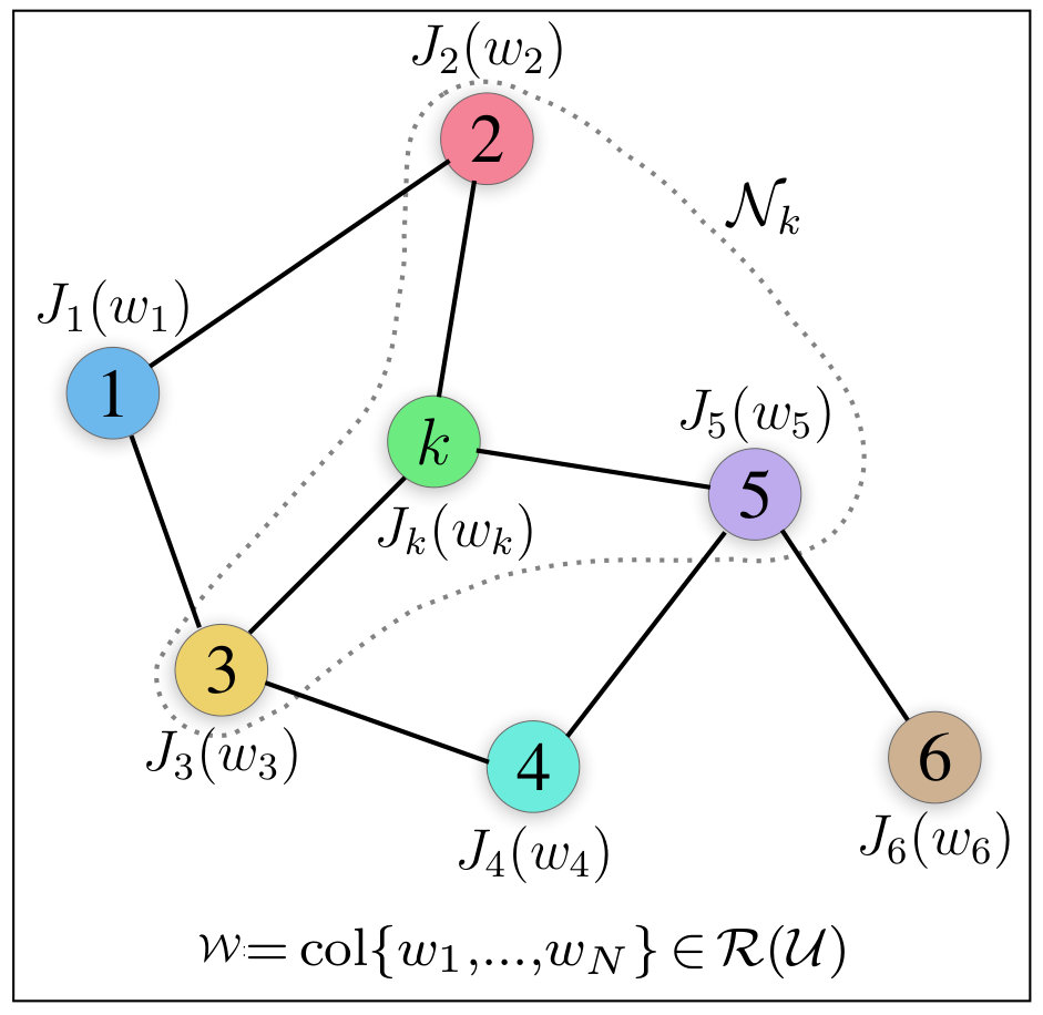 Figure 1
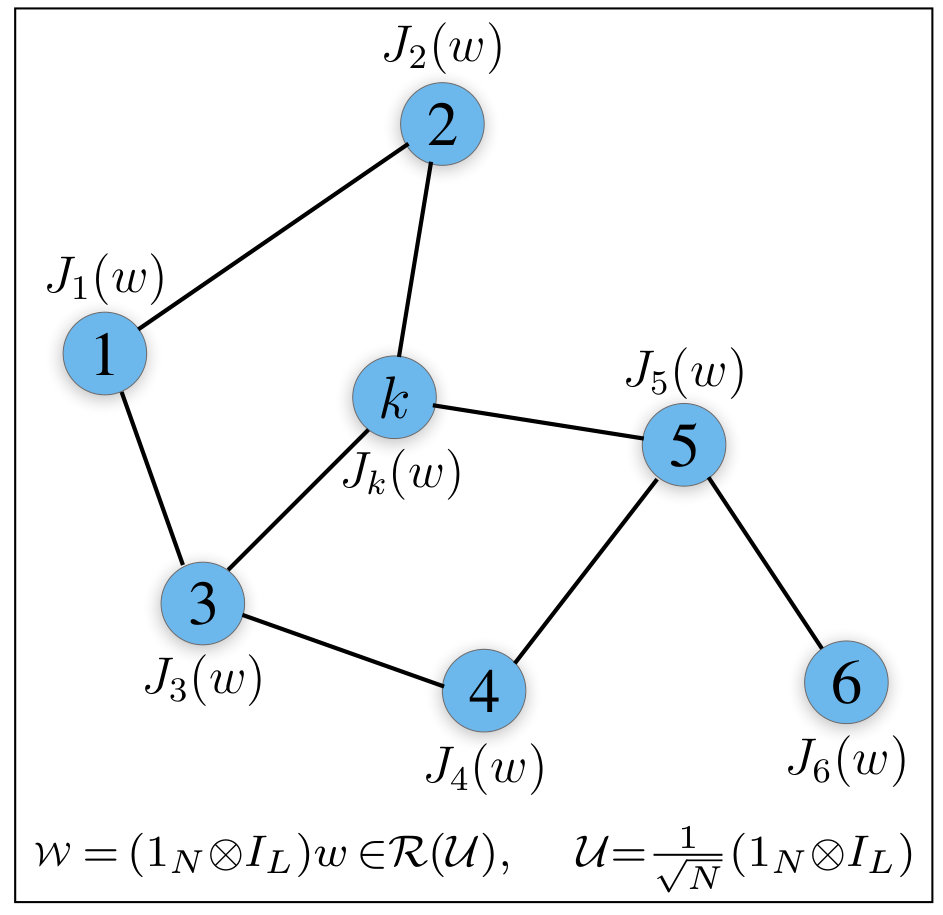 Figure 2
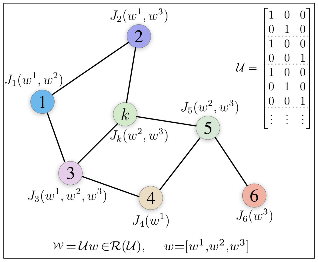 Figure 3
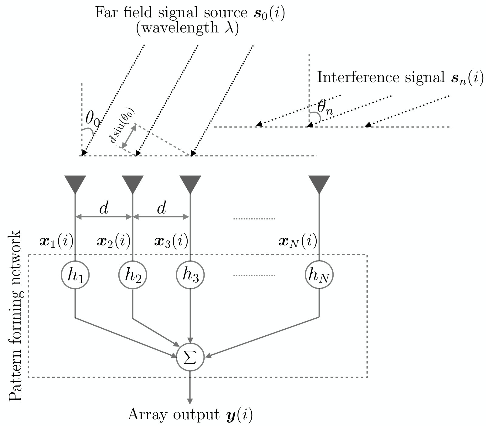 Figure 4
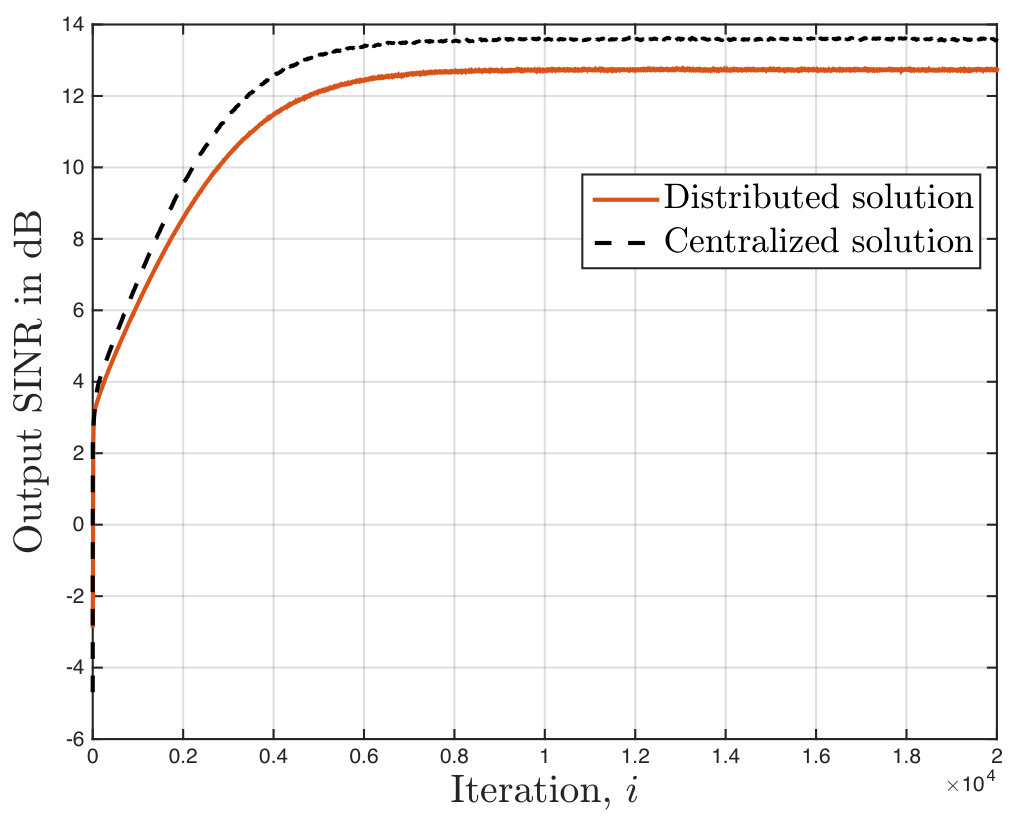 Figure 5
| Neighboring set | Parameter vector | Regressor |
|---|---|---|
Peer Reviews
No public reviews on file for this paper yet. If you reviewed it on a platform where reviews are public (OpenReview, ICLR, NeurIPS, ICML), you can paste yours below so the community can read it here.
Videos
No videos yet. Explain this paper in a talk, walkthrough, or lecture? Add one.
\stackMath
Adaptation and learning over networks under subspace constraints – Part I: Stability Analysis
Roula Nassif*†, , Stefan Vlaski†,‡*, ,
Ali H. Sayed*†*,
† Institute of Electrical Engineering, EPFL, Switzerland
‡ Electrical Engineering Department, UCLA, USA
[email protected] [email protected] [email protected] This work was supported in part by NSF grant CCF-1524250. A short conference version of this work appears in [1].
Abstract
This paper considers optimization problems over networks where agents have individual objectives to meet, or individual parameter vectors to estimate, subject to subspace constraints that require the objectives across the network to lie in low-dimensional subspaces. This constrained formulation includes consensus optimization as a special case, and allows for more general task relatedness models such as smoothness. While such formulations can be solved via projected gradient descent, the resulting algorithm is not distributed. Starting from the centralized solution, we propose an iterative and distributed implementation of the projection step, which runs in parallel with the stochastic gradient descent update. We establish in this Part I of the work that, for small step-sizes , the proposed distributed adaptive strategy leads to small estimation errors on the order of . We examine in the accompanying Part II [2] the steady-state performance. The results will reveal explicitly the influence of the gradient noise, data characteristics, and subspace constraints, on the network performance. The results will also show that in the small step-size regime, the iterates generated by the distributed algorithm achieve the centralized steady-state performance.
Index Terms:
Distributed optimization, subspace projection, gradient noise, stability analysis.
I Introduction
Distributed inference allows a collection of interconnected agents to perform parameter estimation tasks from streaming data by relying solely on local computations and interactions with immediate neighbors. Most prior literature focuses on consensus problems, where agents with separate objective functions need to agree on a common parameter vector corresponding to the minimizer of the aggregate sum of the individual costs, namely,
[TABLE]
where is the cost function at agent , is the number of agents in the network, and is the global parameter vector, which all agents need to agree upon–see Fig. 1 (middle). Each agent seeks to estimate through local computations and communications among neighboring agents without the need to know any of the costs besides their own. Among many useful strategies that have been proposed in the literature [3, 4, 5, 6, 7, 8, 9, 10], diffusion strategies [3, 4, 5] are particularly attractive since they are scalable, robust, and enable continuous learning and adaptation in response to drifts in the location of the minimizer.
However, there exist many network applications that require more complex models and flexible algorithms than consensus implementations since their agents may involve the need to estimate and track multiple distinct, though related, objectives. For instance, in distributed power system state estimation, the local state vectors to be estimated at neighboring control centers may overlap partially since the areas in a power system are interconnected [11, 12]. Likewise, in monitoring applications, agents need to track the movement of multiple correlated targets and to exploit the correlation profile in the data for enhanced accuracy [13, 14]. Problems of this kind, where nodes need to infer multiple, though related, parameter vectors, are referred to as multitask problems. Existing strategies to address multitask problems generally exploit prior knowledge on how the tasks across the network relate to each other [15, 11, 13, 16, 17, 18, 19, 20, 21, 22, 23, 24, 25, 12, 26, 27, 28, 29, 14]. For example, one way to model relationships among tasks is to formulate convex optimization problems with appropriate co-regularizers between neighboring agents [13, 16, 17, 18, 19]. Graph spectral regularization can also be used in order to leverage more thoroughly the graph spectral information and improve the multitask network performance [20]. In other applications, it may happen that the parameter vectors to be estimated at neighboring agents are related according to a set of linear equality constraints [22, 23, 24, 21, 26, 12, 25].
However, in this paper, and the accompanying Part II [2], we consider multitask inference problems where each agent seeks to minimize an individual cost (expressed as the expectation of some loss function), and where the collection of parameter vectors to be estimated across the network is required to lie in a low-dimensional subspace–see Fig. 1 (left). That is, we let denote some parameter vector at node and let denote the collection of parameter vectors from across the network. We associate with each agent a differentiable convex cost , which is expressed as the expectation of some loss function and written as , where denotes the random data. The expectation is computed over the distribution of the data. Let . We consider constrained problems of the form:
[TABLE]
where denotes the range space operator, and is an full-column rank matrix with . Each agent is interested in estimating the -th subvector of . In order to solve (2) iteratively, the gradient projection method can be applied [30]:
[TABLE]
where with the estimate of at iteration and agent , is a small step-size parameter, is the (Wirtinger) complex gradient [4, Appendix A] of relative to (complex conjugate of ), and is the projector onto the -dimensional subspace of spanned by the columns of :
[TABLE]
where we used the fact that is a full-column rank matrix.
We are particularly interested in solving the problem in the stochastic setting when the distribution of the data is generally unknown. This means that the risks and their gradients are unknown. As such, approximate gradient vectors need to be employed. A common construction in stochastic approximation theory is to employ the following approximation at iteration :
[TABLE]
where represents the data observed at iteration . The difference between the true gradient and its approximation is called gradient noise. This noise will seep into the operation of the algorithm and one main challenge is to show that despite its presence, agent is still able to approach asymptotically.
Although the gradient update in (3) and (5) can be performed locally at agent , the projection operation requires a fusion center. To see this, let us introduce an intermediate variable at node :
[TABLE]
After evaluating locally, each agent at each iteration needs to send its estimate to a fusion center, which performs the projection operation in (3) by computing , and then sends the resulting estimates back to the agents. While centralized solutions can be powerful, decentralized solutions are more attractive since they are more robust and respect the privacy policy at each agent [4]. Thus, a second challenge we face in this paper is how to carry out the projection through a distributed network where each node performs local computations and exchanges information only with its neighbors.
We propose in Section II an adaptive and distributed iterative algorithm allowing each agent to converge, in the mean-square-error sense, within from the solution of (2), for sufficiently small . Conditions on the network topology and signal subspace ensuring the feasibility of a distributed implementation are provided. We also show how some well-known network optimization problems, such as consensus optimization [3, 4, 5] and multitask smooth optimization [16], can be recast in the form (2) and addressed with the strategy proposed in this paper. The analysis in Section III of this Part I shows that, for sufficiently small , the proposed adaptive strategy leads to small estimation errors on the order of the small step-size. Building on the results of this Part I, we shall derive in Part II [2] a closed-form expression for the steady-state network mean-square-error performance. This closed form expression will reveal explicitly the influence of the data characteristics (captured by the second-order properties of the costs and second-order moments of the gradient noises) and subspace constraints (captured by ), on the network performance. The results will also show that, in the small step-size regime, the iterates generated by the distributed implementation achieve the centralized steady-state performance. For illustration purposes, distributed sub-optimal beamforming is considered in Section IV of this Part I.
Notation: All vectors are column vectors. Random quantities are denoted in boldface. Matrices are denoted in capital letters while vectors and scalars are denoted in lower-case letters. We use the symbol to denote matrix transpose, the symbol to denote matrix complex-conjugate transpose, and the symbol to denote trace operator. The symbol forms a matrix from block arguments by placing each block immediately below and to the right of its predecessor. The operator stacks the column vector entries on top of each other. The symbol denotes the Kronecker product. The identity matrix is denoted by .
II Distributed inference under subspace constraints
We move on to propose and study a distributed solution for solving (2) with a continuous adaptation mechanism. The solution must rely on local computations and communications with immediate neighborhood, and operate in real-time on streaming data. To proceed with the analysis, one of the challenges we face is that the projection in (3) requires non-local exchange of information. Our strategy is to replace the projection matrix in (3) by an matrix that satisfies the following conditions:
[TABLE]
where denotes the -th block of of dimension and denotes the neighborhood of agent , i.e., the set of nodes connected to agent by an edge. The sparsity condition (8) characterizes the network topology and ensures local exchange of information at each time instant . By replacing the projector in (3) by and the true gradients by their stochastic approximations, we obtain the following distributed adaptive solution at each agent :
[TABLE]
where we used condition (8), and where is an intermediate estimate and is the estimate of at agent and iteration . As we shall see in Section III, condition (7) helps ensure convergence toward the optimum. Necessary and sufficient conditions for the matrix equation (7) to hold are given in the following lemma.
Lemma 1**.**
(Necessary and sufficient conditions for (7))*
The matrix equation (7) holds, if and only if, the following conditions on the projector and the matrix are satisfied:*
[TABLE]
where denotes the spectral radius of its matrix argument. It follows that any satisfying condition (7) has one as an eigenvalue with multiplicity , and all other eigenvalues are strictly less than one in magnitude.
Proof.
See Appendix A. The arguments are along the lines developed in [31] for distributed averaging with proper adjustments to handle general subspace constraints. ∎
Note that conditions (10)–(12) appeared previously (with proof omitted) in the context of distributed denoising in wireless sensor networks [29]. In such problems, the sensors are observing -dimensional signal, with each entry of the signal corresponding to one sensor. Using the prior knowledge that the observed signal belongs to a low-dimensional subspace, the sensor task is to denoise the corresponding entry of the signal by projecting in a distributed iterative manner onto the signal subspace in order to improve the error variance. However, in this work, we consider the more general problem of distributed inference over networks.
If we replace by (4), multiply both sides of (10) by , and multiply both sides of (11) by , conditions (10) and (11) reduce to:
[TABLE]
Conditions (13) and (14) state that the columns of are right and left eigenvectors of associated with the eigenvalue . Together with these two conditions, condition (12) means that has eigenvalues at one, and that all other eigenvalues are strictly less than one in magnitude.
In the following, we discuss how some well-known network optimization problems can be recast in the form (2) and addressed with strategies in the form of (9).
Remark 1. (Distributed consensus optimization). Let for all agents. If we set in (2) and where is the vector of all ones, then solving problem (2) will be equivalent to solving the well-known consensus problem (1). Different algorithms for solving (1) over strongly-connected networks have been proposed [3, 4, 5, 7, 6, 8, 9]. By picking any doubly-stochastic matrix satisfying:
[TABLE]
the diffusion strategy for instance takes the form [3, 4, 5]:
[TABLE]
Observe that this strategy can be written in the form of (9) with and . It can be verified that, when satisfies (15) over a strongly connected network, the matrix will satisfy (8), (13), (14), and (12). ∎
Remark 2. (Distributed coupled optimization). Similarly, with a proper selection of , multitask inference problems with overlapping parameter vectors [23, 22, 24] can also be recast in the form (2). This scenario is illustrated in Fig. 1 (right). In this example, agent is influenced by only a subset of the entries of a global and seeks to estimate . For a given variable and any two arbitrary agents containing in their costs, it is assumed that the network topology is such that there exists at least one path linking one agent to the other [23]. By properly selecting the matrix , the network vector can be written as and, therefore, distributed coupled optimization can be recast in the form (2). It can be verified that the coupled diffusion strategy proposed in [23] for solving this problem can be written in the form of (9) and that the (doubly-stochastic) matrix in [23] satisfies conditions (7) and (8). ∎
Remark 3. (Distributed optimization under affine constraints). Several existing works consider (distributed or offline) variations of the following problem [27, 26, 28]:
[TABLE]
where is an full-column rank matrix and is an column vector. It turns out that the online distributed strategy proposed in this work can be used to solve (17) for general constraints that are not necessarily local. To see this, we first note that the gradient projection method can be applied to solve (17) [30]:
[TABLE]
where and . Since is a projection matrix, it can be decomposed as with the orthonormal eigenvectors of associated with the eigenvalues at one, and thus can be replaced by with . Therefore, solution (18) has a form similar to the earlier solution (3) with the rightmost term in (18) absent from (3). Following the same line of reasoning that led to (9), we can similarly obtain the following distributed adaptive solution for solving (17):
[TABLE]
where is the -th sub-vector of corresponding to node (see Appendix B), and is a properly selected matrix satisfying conditions (7) and (8). Although algorithm (19) is different than (9) due to the presence of the constant term , the mean-square-error analyzes of both algorithms are the same, as we shall see in Section III. In Section IV, we shall apply (19) to solve linearly constrained beamforming [32, 33].∎
Remark 4. (Distributed inference under smoothness). Let for all agents. In such problems, each agent in the network has an individual cost to minimize subject to a smoothness condition over the graph. The smoothness requirement softens the transition in the tasks among neighboring nodes and can be measured in terms of a quadratic form of the graph Laplacian [16]:
[TABLE]
where with denoting the graph Laplacian. The matrix is an symmetric weighted adjacency matrix with if and otherwise. The smaller is, the smoother the signal on the graph is. Since is symmetric positive semi-definite, it can be decomposed as where with the non-negative eigenvalues ordered as and is the matrix of orthonormal eigenvectors. When the graph is connected, there is only one zero eigenvalue with corresponding eigenvector [34]. Using the eigenvalue decomposition , can be written as:
[TABLE]
where and . Given that , the above expression shows that is considered to be smooth if corresponding to large is negligible. Thus, for a smooth , will be equal to with . By choosing where , the smooth signal will be in the range space of since it can be written as with . Therefore, distributed inference problems under smoothness can be recast in the form (2).∎
Before proceeding, note that, in some cases, one may find a family of matrices satisfying conditions (12), (13), and (14) under the sparsity constraints (8). For example, in consensus optimization described in Remark 1 where , by ensuring that the underlying graph is strongly connected and by choosing any doubly-stochastic satisfying the sparsity constraints, the resulting matrix will satisfy the required conditions. The same observation holds for coupled optimization problems described in Remark 2. Several policies for designing locally doubly-stochastic matrices have been proposed in the literature [3, 4, 5]. For more general , designing an satisfying conditions (7) and (8) can be written as the following feasibility problem:
[TABLE]
which is challenging in general. Not all network topologies satisfying (8) guarantee the existence of an satisfying condition (7). The higher the dimension of the signal subspace is, the greater the graph connectivity has to be. In the works [1, 29], it is assumed that the sparsity constraints (8) and the signal subspace lead to a feasible problem. That is, it is assumed that problem (22) admits at least one solution. As a remedy for the violation of such assumption, one may increase the network connectivity by increasing the transmit power of each node, i.e., adding more links [29]. In the accompanying Part II [2], we shall relax the feasibility assumption by considering the problem of finding an that minimizes the number of edges to be added to the original topology while satisfying the constraints (12), (13), and (14). In this case, if the original topology leads to a feasible solution, then no links will be added. Otherwise, we assume that the designer is able to add some links to make the problem feasible.
In the following section, we consider that a feasible (topology) is computed by the designer and that its blocks are provided to agent in order to run algorithm (9). We shall study the performance of (9) in the mean-square-error sense. We shall consider the general complex case, in addition to the real case, since complex-valued combination matrix and data are important in several applications, as will be the case in the distributed beamforming application considered later in Section IV.
III Stability analysis
In this Part I, we shall establish mean-square-error stability by showing that, for each agent , the error variance relative to enters a bounded region whose size is in the order of , namely, . Then, building on this result, we will assess in the accompanying Part II [2] the size of this mean-square error by deriving closed-form expression for the network mean-square-deviation (MSD) defined by [4]:
[TABLE]
where . In this way, we will be able to conclude that distributed strategies of the form (9) with small step-size are able to lead to reliable performance even in the presence of gradient noise. We will be able also to conclude that the iterates generated by the distributed implementation achieve the centralized steady-state performance.
As explained in [4, Chap. 8], in the general case where are not necessarily quadratic in the (complex) variable , we need to track the evolution of both quantities and in order to examine how the network is performing. Since is real valued, the evolution of the complex conjugate iterates is given by:
[TABLE]
Representations (9) and (24) can be grouped together into a single set of equations by introducing extended vectors of dimensions as follows:
[TABLE]
Therefore, when the data is complex, extended vectors and matrices need to be introduced in order to analyze the network evolution. The arguments and results presented in the analysis are applicable to both cases of real and complex data through the use of data-type variable defined in Table I. When the data is real-valued, the complex conjugate transposition should be replaced by the real transposition. Table I lists a couple of variables and symbols that will be used in the sequel for both real and complex data cases. The superscript “” is used to refer to extended quantities. Although in the real data case no extended quantities should be introduced, we use the superscript “” for both data cases for compactness of notation.
III-A Modeling conditions
We analyze (9) under conditions (8), (12), (13), and (14) on , and the following assumptions on the risks and on the gradient noise processes defined as:
[TABLE]
Before proceeding, we introduce the Hermitian Hessian matrix functions [4, Appendix B]:
[TABLE]
Note that, when , we have:
[TABLE]
where is a permutation matrix given by:
[TABLE]
This matrix consists of blocks with -th block given by:
[TABLE]
for and .
Assumption 1**.**
(Conditions on aggregate and individual costs).*
The individual costs are assumed to be twice differentiable and convex such that:*
[TABLE]
where for . It is further assumed that, for any , satisfies:
[TABLE]
for some positive parameters . The data-type variable and the matrix are defined in Table I.
Condition (38) ensures that problem (2), which can be rewritten as:
[TABLE]
has a unique minimizer . This is due to the fact that the Hessian of , which is given by:
[TABLE]
is positive definite under condition (38).
Assumption 2**.**
(Conditions on gradient noise).*
The gradient noise process defined in (26) satisfies for any and for all :*
[TABLE]
for some , , and where denotes the filtration generated by the random processes for all and .
As explained in [3, 4, 5], these conditions are satisfied by many objective functions of interest in learning and adaptation such as quadratic and logistic risks. Condition (44) essentially states that the gradient vector approximation should be unbiased conditioned on the past data, which is a reasonable condition to require. Condition (47) states that the second-order moment of the gradient noise process should get smaller for better estimates, since it is bounded by the squared-norm of the iterate. Conditions (45) and (46) state that the gradient noises across the agents are uncorrelated and second-order circular.
Without loss of generality, we shall introduce the following assumption on the matrix 111This assumption is not restrictive since for any full-column rank matrix with , we can generate by using, for example, the Gram-Schmidt process [35, pp. 15], a semi-unitary matrix that spans the same -dimensional subspace of as , i.e., ..
Assumption 3**.**
(Condition on ).*
The full-column rank matrix is assumed to be semi-unitary, i.e., its column vectors are orthonormal and .*
Before proceeding, we introduce an block matrix whose -th block is defined in Table I. This matrix will appear in our subsequent study. Observe that in the real data case, , and that in the complex data case, can be seen as an extended version of the combination matrix . The next statement exploits the eigen-structure of that will be useful for establishing the mean-square stability.
Lemma 2**.**
(Jordan canonical decomposition).*
Under Assumption 3, the combination matrix satisfying conditions (13), (14), and (12) admits a Jordan canonical decomposition of the form:*
[TABLE]
with:
[TABLE]
where is a Jordan matrix with the eigenvalues (which may be complex but have magnitude less than one) on the diagonal and on the super-diagonal. It follows that the matrix defined in Table I admits a Jordan decomposition of the form:
[TABLE]
with
[TABLE]
where , and are defined in Table I. Since , the following relations hold:
[TABLE]
Proof.
See Appendix C. ∎
III-B Network error vector recursion
Let denote the error vector at node :
[TABLE]
Consider first the complex data case. Using (26) and the mean-value theorem [36, pp. 24], [4, Appendix D], we can express the stochastic gradient vectors appearing in (25) as follows:
[TABLE]
where:
[TABLE]
and , , and are defined in Table I with:
[TABLE]
Subtracting from both sides of (25) and by introducing the following extended vectors and matrices, which collect quantities from across the network:
[TABLE]
we can show that the network weight error vector in (57) evolves according to the following dynamics:
[TABLE]
where is defined in Table I and where we used (54) and the fact that
[TABLE]
since is the solution of problem (2), and thus:
[TABLE]
For real data, the model can be simplified since we do not need to track the evolution of the complex conjugate . Although we use the notation “” for the quantities in the above recursion, it is to be understood that the extended quantities should be replaced by the quantities as in Table I.
The stability analysis of recursion (62) is facilitated by transforming it to a convenient basis using the Jordan decomposition of in Lemma 2. Multiplying both sides of (62) from the left by and introducing the transformed iterates and variables:
[TABLE]
we obtain from Lemma 2:
[TABLE]
where
[TABLE]
Recursions (LABEL:eq:_error_recursion_for_wbi) and (LABEL:eq:_error_recursion_for_wci) can be written more compactly as:
[TABLE]
The zero entry in (77) is due to the fact that
[TABLE]
since the constrained optimization problem (2) can be written alternatively as:
[TABLE]
The Lagrangian associated with problem (90) is given by:
[TABLE]
where is the vector of Lagrange multipliers. From the optimality conditions, we obtain the following condition on :
[TABLE]
where we used the fact that is real valued and where and are given by (61) and (36), respectively. In the real data case, by multiplying both sides of the previous relation by , we obtain . For complex data, by multiplying both sides of the previous equation by with defined in Table I, we obtain . Now, considering both real and complex data cases, we arrive at (89).
Remark 5. Regarding algorithm (19), it can be verified that the weight error vector will end up evolving according to recursion (62). The constant driving terms will disappear when subtracting from both sides of (19) since satisfies the following relation:
[TABLE]
where we used the fact that the optimal solution in (17) verifies:
[TABLE]
By rewriting the constraint in (17) as and repeating similar arguments as (90)–(100), we can show that . Therefore, the transformed iterates and in (69) will continue to evolve according to recursions (LABEL:eq:_error_recursion_for_wbi) and (LABEL:eq:_error_recursion_for_wci). ∎
In the following, we shall establish the mean-square-error stability of algorithm (9). In the accompanying Part II, we will derive a closed-form expression for the network MSD defined by (23). The derivation is demanding. However, the arguments are along the lines developed in [4, Chaps. 9–11] for standard diffusion (16) with proper adjustments to handle possibly complex valued block matrices satisfying conditions (7) and (8) and the subspace constraints.
III-C Mean-square-error stability
Theorem 1**.**
(Network mean-square-error stability).*
Consider a network of agents running the distributed strategy (9) with a matrix satisfying conditions (13), (14), and (12) and satisfying Assumption 3. Assume the individual costs, , satisfy the conditions in Assumption 1. Assume further that the first and second-order moments of the gradient noise process satisfy the conditions in Assumption 2. Then, the network is mean-square-error stable for sufficiently small step-sizes, namely, it holds that:*
[TABLE]
for small enough .
Proof.
See Appendix D. ∎
IV Distributed linearly constrained minimum variance (LCMV) beamformer
Consider a uniform linear array (ULA) of antennas, as shown in Fig. 2. A desired narrow-band signal from far field impinges on the array from known direction of arrival (DOA) along with two uncorrelated interfering signals from DOAs , respectively. We assume that the DOA of is roughly known. The received signal at the array is therefore modeled as:
[TABLE]
where is an vector that collects the received signals at the antenna elements, are array manifold vectors (steering vectors) for the desired and interference signals, and is the additive noise vector at time . With the first element as the reference point, the array manifold vector is given by [32], with where denotes the spacing between two adjacent antenna elements, and denotes the wavelength of the carrier signal. The antennas are assumed spaced half a wavelength apart, i.e., .
Beamforming problems generally deal with the design of a weight vector in order to recover the desired signal from the received data [32, 33]. The narrowband beamformer output can be expressed as . Among many possible criteria, we use the linearly-constrained-minimum-variance (LCMV) design, namely,
[TABLE]
where is an matrix and is a vector, in order to suppress the influence of the perturbation on the output while preserving the signal component. Since the DOAs of is known and the DOA of is roughly known, matrix can be chosen as , and the vector as . In this way, we set unit response to the direction of the desired signal so that passes through the array without distortion.
In a distributed setting, the objective of agent (antenna element) is to estimate , the -th component of in (105). Neighboring agents are allowed to exchange their observations . To each agent , we associate a neighborhood set , an parameter vector , and an regression vector , defined in Table II depending on the node location on the array. Observe that the parameter controls the network topology. For example, corresponds to a fully connected network setting. We associate with each agent a cost Instead of solving (105), we propose to solve:
[TABLE]
where the equality constraint merges the equality constraint in (105) and the equality constraints that need to be imposed on the parameter vectors at neighboring nodes in order to achieve equality between common entries (see Table II). Let denote the binary connection matrix with if , and [math] otherwise. Under the consensus constraints, it can be shown that:
[TABLE]
where is an matrix with and is the element-wise product. Therefore, collecting observations from neighboring nodes allows partial covariance matrix computation, which will be used in optimization. For the partial covariance to converge to the true covariance in (105), we need to set in order to have . Note that, two main classes of distributed beamforming appear in the literature [37]. In the first class, which is considered here, the covariance matrix is approximated to form distributed implementations [38, 39, 40, 37] leading to sub-optimal beamformers. In the second class, the proposed beamformers obtain statistical optimality but do so at the expense of restricting the topology of the underlying network [41]. Different from [38], the current distributed solution preserves convexity and is scalable since nodes exchange and compute sub-vectors with instead of vectors.
Algorithm (9) can be applied to solve (106). The signals are i.i.d. zero-mean complex Gaussian random variables with variance . The additive noise is zero-mean complex Gaussian with covariance (). We set . The complex combination matrix is set as the solution of the feasibility problem (22) with the constraint replaced by () and the constraint added222These changes make the problem convex–see [2, Sec. 3] for further details.. The resulting problem is solved via CVX package [42]. Note that the distributed implementation is feasible in this example. We set . The output signal-to-interference-plus-noise ratio (SINR) given by with is illustrated in Fig. 2 (right). The dashed black curve is the beampattern obtained by the centralized, also known as the constrained LMS [33], algorithm (). The results are averaged over Monte-Carlo runs. We observe that the distributed solution performs well compared to the centralized implementation.
V Conclusion
In this work, we considered inference problems over networks where agents have individual parameter vectors to estimate subject to subspace constraints that require the parameters across the network to lie in low-dimensional subspaces. Based on the gradient projection algorithm, we proposed an iterative and distributed implementation of the projection step, which runs in parallel with the stochastic gradient descent update. We showed that, for small step-size parameter, the network is able to approach the minimizer of the constrained problem to arbitrarily good accuracy levels.
Appendix A Proof of Lemma 1
First we prove sufficiency by proving that if is a projection matrix and satisfies conditions (10), (11), and (12), then the matrix equation (7) holds. If satisfies (10) and (11), then:
[TABLE]
where we used the fact that since is a projector. Applying condition (12) and using the fact that for any matrix , if and only if , we obtain the desired convergence (7).
To prove necessity, we shall prove that every time we have (7), we will have a projection matrix and conditions (10), (11), and (12) on satisfied. We use the fact that exists if, and only if, there is a non singular matrix such that [43]:
[TABLE]
where the spectral radius of is less than one. Let be the columns of and be the rows of . Then, we have:
[TABLE]
From the left hand-side of (7) and (119), we obtain:
[TABLE]
Observe from (113) that one is an eigenvalue of with multiplicity and are the associated right and left eigenvectors. Thus, from (122), we obtain:
[TABLE]
and equations (10) and (11) hold. Moreover, from (113) and (122), we obtain:
[TABLE]
which is condition (12). Finally, from (122), we have:
[TABLE]
Thus, is a projector, which completes the necessity proof.
Since each is a rank-one matrix and their sum has rank , the matrix must have rank . Since the rank of is equal to , we obtain from (122) . Thus, the matrix has eigenvalues at one and all other eigenvalues are strictly less than one.
Appendix B Driving term in algorithm (19)
Let denote an vector distributed across the network. In order to justify the choice of in (19), we consider the problem of finding the projection in a distributed and iterative manner through a linear iteration of the form:
[TABLE]
where satisfies (7), (8) and is a properly chosen matrix ensuring convergence toward . Starting from and iterating the above recursion, we obtain:
[TABLE]
If we let on both sides of (132), we find:
[TABLE]
For to be equal to , in (131) must be chosen such that . In the following, we show that ensures convergence. From the Jordan canonical form of introduced in (49), we have:
[TABLE]
If we multiply both terms and compute the infinite sum in (133), we obtain:
[TABLE]
where we used the fact that since .
Now, since and , we obtain , which justifies the choice in (19).
Appendix C Proof of Lemma 2
We start by noting that the matrix satisfying conditions (13), (14), and (12) admits a Jordan canonical decomposition of the form:
[TABLE]
where the matrix consists of Jordan blocks, with each one of them having the form (say for a Jordan block of size ):
[TABLE]
where the eigenvalue may be complex but has magnitude less than one. Let with any small positive number independent of . The matrix in (148) can be written alternatively as:
[TABLE]
where
[TABLE]
and where the matrix consists of Jordan blocks, with each one of them having a form similar as (152) with appearing on the upper diagonal instead of , and where the eigenvalue may be complex but has magnitude less than one. Obviously, since , it holds that:
[TABLE]
and where from Assumption 3.
Now, let us consider the extended version of the matrix , namely, , which is an block matrix whose -th block is defined in Table I. In the real data case, we have . In the complex data case, it can be verified that is similar to the block diagonal matrix:
[TABLE]
according to:
[TABLE]
where is the permutation matrix defined by (36). Using (153), we can rewrite the second block in (163) as:
[TABLE]
where and
[TABLE]
Now, by replacing (153) and (165) into (163), and by introducing the extended block diagonal matrices:
[TABLE]
we find that the matrix has a Jordan decomposition of the form:
[TABLE]
Let us again introduce a permutation matrix given by:
[TABLE]
The matrix in (172) can be written alternatively as:
[TABLE]
where the matrix is block diagonal defined in (51). Returning now to , and using (164) and (178), we find that the matrix has a Jordan decomposition of the form:
[TABLE]
where and are defined by:
[TABLE]
in terms of the permutation matrices and in (35), (177) and the block diagonal matrix in (170). By properly evaluating these matrices, we arrive at (51).
Appendix D Proof of Theorem 1
We consider the transformed variables and in (69). Conditioning both sides on , computing the conditional second-order moments, using the conditions from Assumption 2 on the gradient noise process, and computing the expectations again, we get:
[TABLE]
and
[TABLE]
By applying Jensen’s inequality to the convex function , we can bound the first term on the RHS of (181) as follows:
[TABLE]
for any arbitrary positive number . By Assumption 1, the Hermitian matrix defined in (55) can be bounded as follows:
[TABLE]
Using the fact that the integral of a matrix is the matrix of the integrals, and the linear property of integration, the Hermitian block in (78) can be rewritten as:
[TABLE]
and, therefore, from Assumption 1, can be bounded as follows:
[TABLE]
for some positive constants and that are independent of and . In terms of the induced matrix norm (i.e., maximum singular value), we obtain:
[TABLE]
and, therefore,
[TABLE]
for some positive constant that is independent of and .
Similarly, using the induced matrix norm (i.e., maximum singular value), we can bound as follows:
[TABLE]
for some positive constant and where we used the fact that .
Substituting (LABEL:eq:_first_term_on_the_RHS) into (181), and using (187), (188), we get:
[TABLE]
We select (for sufficiently small ). Then, the previous inequality can be written as:
[TABLE]
We repeat similar arguments for the second variance relation (182). Using Jensen’s inequality again, we obtain:
[TABLE]
for any arbitrary positive number . In (a) we used the fact that the block diagonal matrix defined in Table I satisfies:
[TABLE]
Expression (192) can be established by using similar arguments as in [4, pp. 516] and the fact that . In (b), we used the fact that , and thus, can be selected small enough to ensure . We then selected .
Using Jensen’s inequality, the second term on the RHS of (191) can be bounded as follows:
[TABLE]
Following similar arguments as in (188), we can show that:
[TABLE]
for some positive constants and . Substituting (193) into (191) and (191) into (182), and using (194), we obtain:
[TABLE]
From (77), we have:
[TABLE]
where we used the fact that from Lemma 2. Since in (61) is defined in terms of the gradient and since is twice differentiable, then is bounded and we obtain . For the noise terms in (190) and in (195), we have:
[TABLE]
where is a positive constant independent of and given by . In terms of the variances of the individual noise processes, , we have . For each , we have from Assumption 2 and Jensen’s inequality:
[TABLE]
where and . The term can thus be bounded as follows:
[TABLE]
where , , and . Substituting into (197), we get:
[TABLE]
Using this bound in (190) and (195), we obtain:
[TABLE]
[TABLE]
We can combine (200) and (201) into a single inequality recursion:
[TABLE]
where is given by:
[TABLE]
and where , , , , , and . Now, using the property that the spectral radius of a matrix is upper bounded by its norm norm, we obtain:
[TABLE]
Since is independent of , and since and are small positive numbers that can be chosen arbitrarily small and independently of each other, it is clear that the RHS of the above expression can be made strictly smaller than one for sufficiently small and . In that case so that is stable. Moreover, it holds that:
[TABLE]
Now, by iterating (208) we arrive at:
[TABLE]
from which we conclude that and . Therefore,
[TABLE]
The reference list from the paper itself. Each links out to its DOI / PubMed record.
- 1[1] R. Nassif, S. Vlaski, and A. H. Sayed, “Distributed inference over networks under subspace constraints,” in Proc. IEEE Int. Conf. Acoust., Speech, and Signal Process. , Brighton, UK, May 2019, pp. 1–5.
- 2[2] R. Nassif, S. Vlaski, and A. H. Sayed, “Adaptation and learning over networks under subspace constraints – Part II: Performance analysis,” Submitted for publication. , May 2019.
- 3[3] A. H. Sayed, S. Y. Tu, J. Chen, X. Zhao, and Z. J. Towfic, “Diffusion strategies for adaptation and learning over networks,” IEEE Signal Process. Mag. , vol. 30, no. 3, pp. 155–171, 2013.
- 4[4] A. H. Sayed, “Adaptation, learning, and optimization over networks,” Foundations and Trends in Machine Learning , vol. 7, no. 4-5, pp. 311–801, 2014.
- 5[5] A. H. Sayed, “Adaptive networks,” Proc. IEEE , vol. 102, no. 4, pp. 460–497, Apr. 2014.
- 6[6] D. Bertsekas, “A new class of incremental gradient methods for least squares problems,” SIAM J. Optim. , vol. 7, no. 4, pp. 913–926, 1997.
- 7[7] A. Nedic and A. Ozdaglar, “Distributed subgradient methods for multi-agent optimization,” IEEE Trans. Autom. Control , vol. 54, no. 1, pp. 48–61, Jan. 2009.
- 8[8] A. G. Dimakis, S. Kar, J. M. F. Moura, M. G. Rabbat, and A. Scaglione, “Gossip algorithms for distributed signal processing,” Proc. IEEE , vol. 98, no. 11, pp. 1847–1864, Nov. 2010.