Revisiting the new-physics interpretation of the $b\to c\tau\nu$ data
Rui-Xiang Shi, Li-Sheng Geng, Benjam\'in Grinstein, Sebastian J\"ager,, and Jorge Martin Camalich

TL;DR
This paper reevaluates new-physics explanations for anomalies in semileptonic B decays, incorporating recent Belle data, and identifies key observables that can distinguish among different theoretical models.
Contribution
It provides an updated analysis of new-physics scenarios explaining B decay anomalies, highlighting the roles of various operators and the importance of specific measurements.
Findings
Left-handed currents and tensor contributions are favored explanations.
Pure right-handed and scalar models are disfavored by collider and lifetime constraints.
Tau polarization measurements can effectively discriminate among new-physics scenarios.
Abstract
We revisit the status of the new-physics interpretations of the anomalies in semileptonic decays in light of the new data reported by Belle on the lepton-universality ratios using the semileptonic tag and on the longitudinal polarization of the in , . The preferred solutions involve new left-handed currents or tensor contributions. Interpretations with pure right-handed currents are disfavored by the LHC data, while pure scalar models are disfavored by the upper limits derived either from the LHC or from the lifetime. The observable also gives an important constraint leading to the exclusion of large regions of parameter space. Finally, we investigate the sensitivity of different observables to the various scenarios and conclude that a measurement of the tau polarization in the decay mode would…
Click any figure to enlarge with its caption.
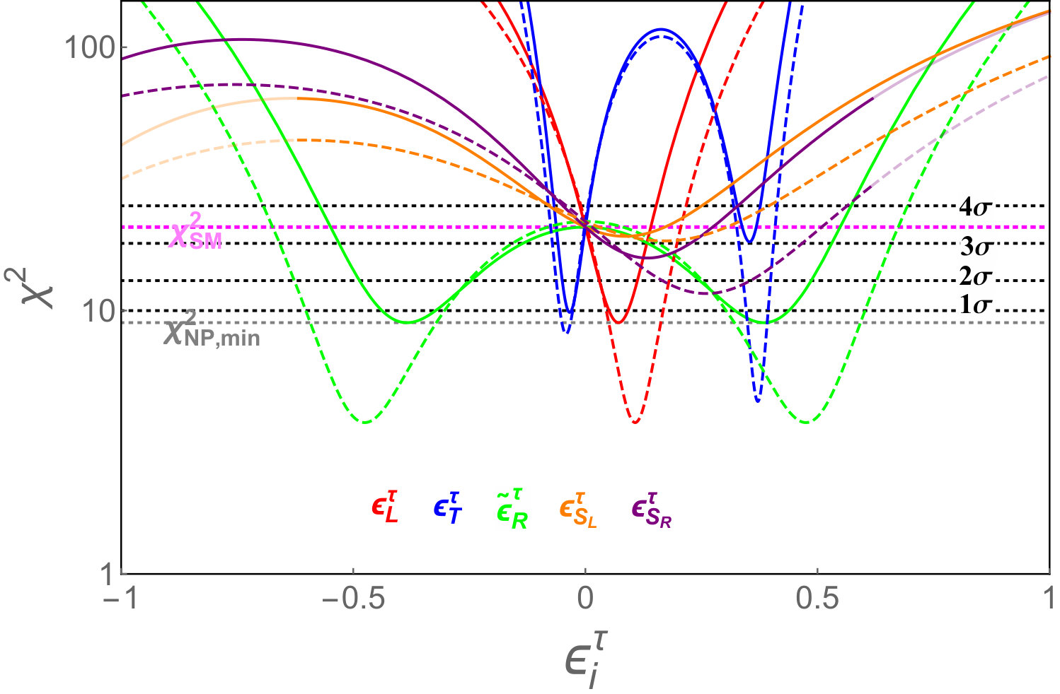 Figure 1
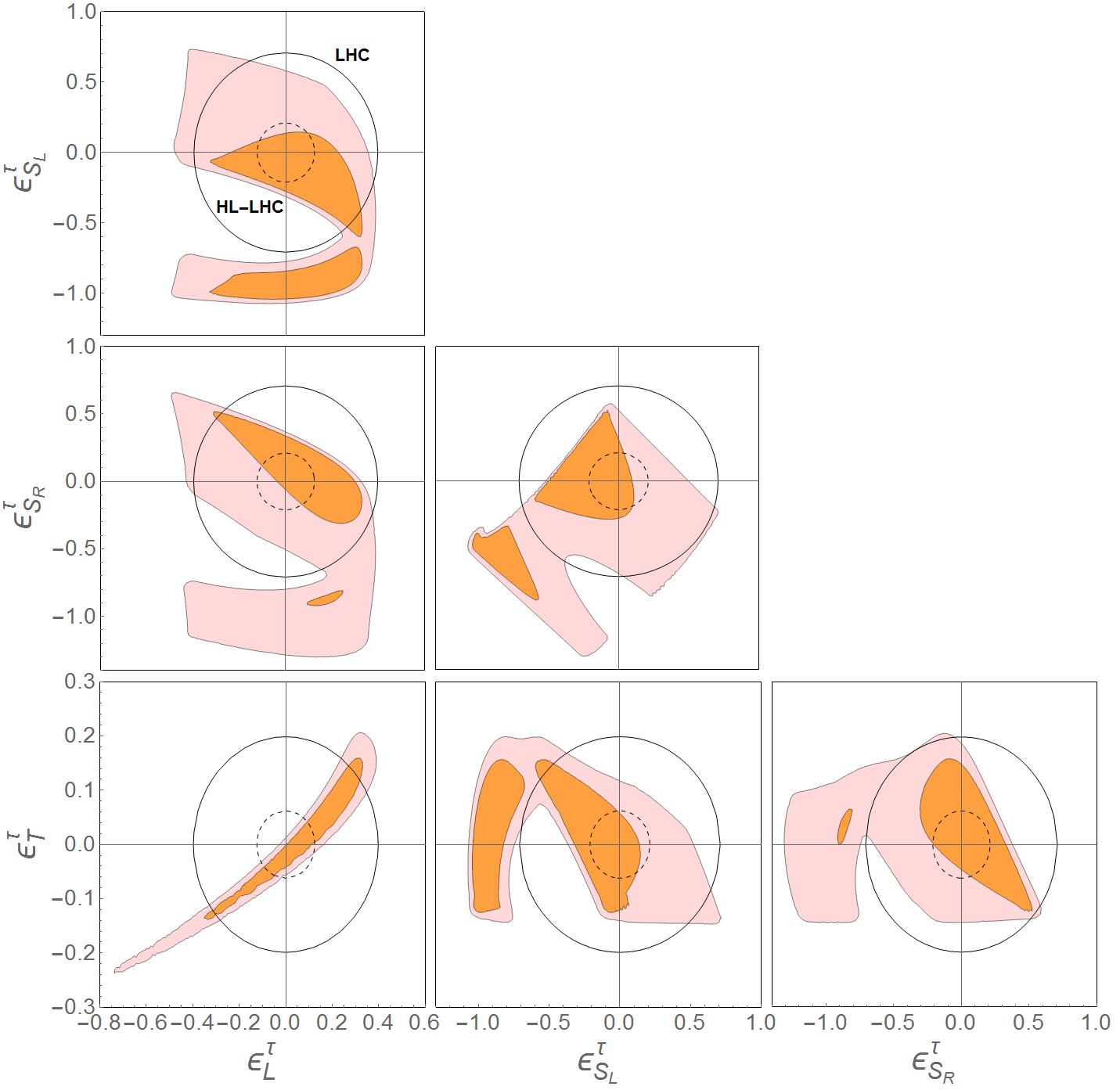 Figure 2
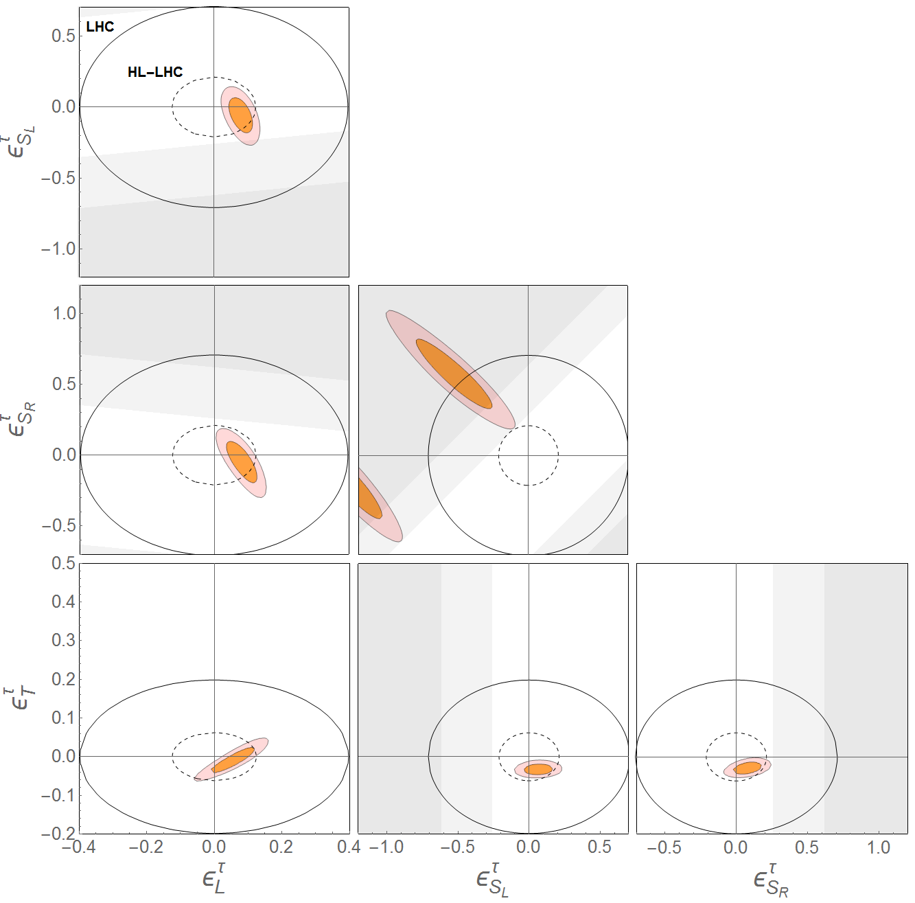 Figure 3
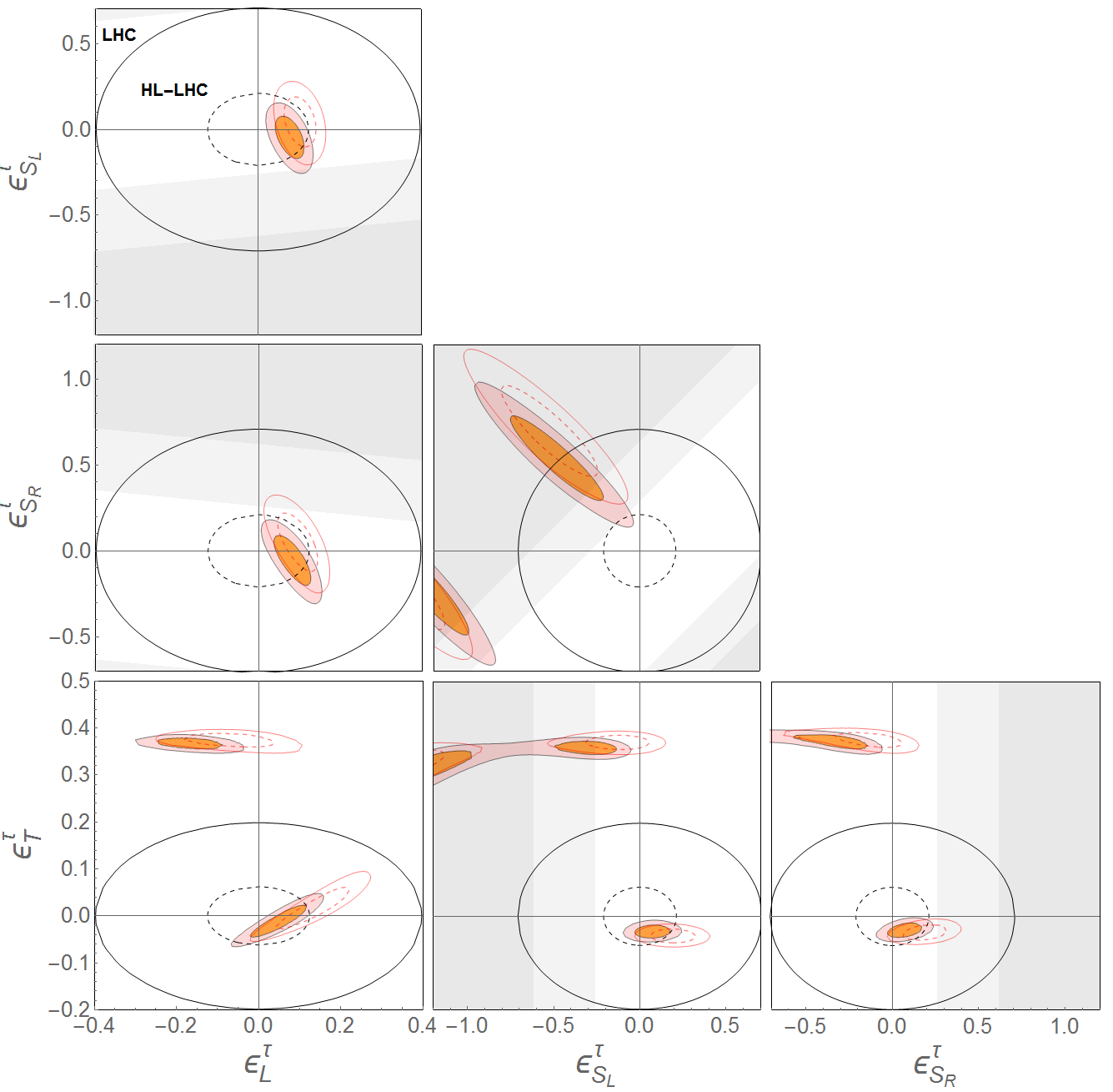 Figure 4
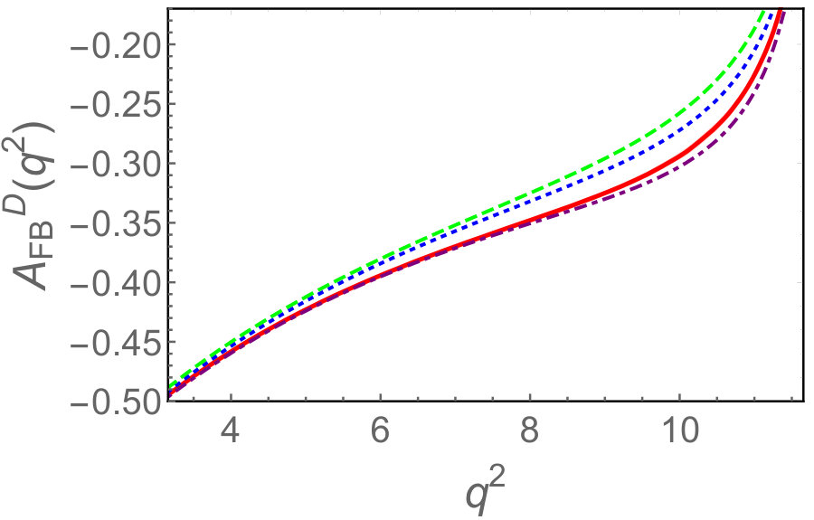 Figure 5
 Figure 6
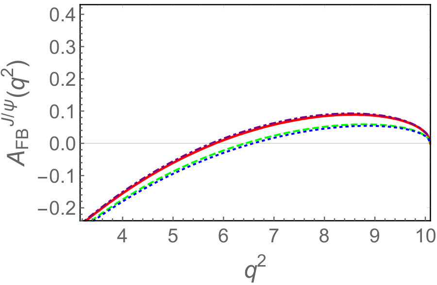 Figure 7
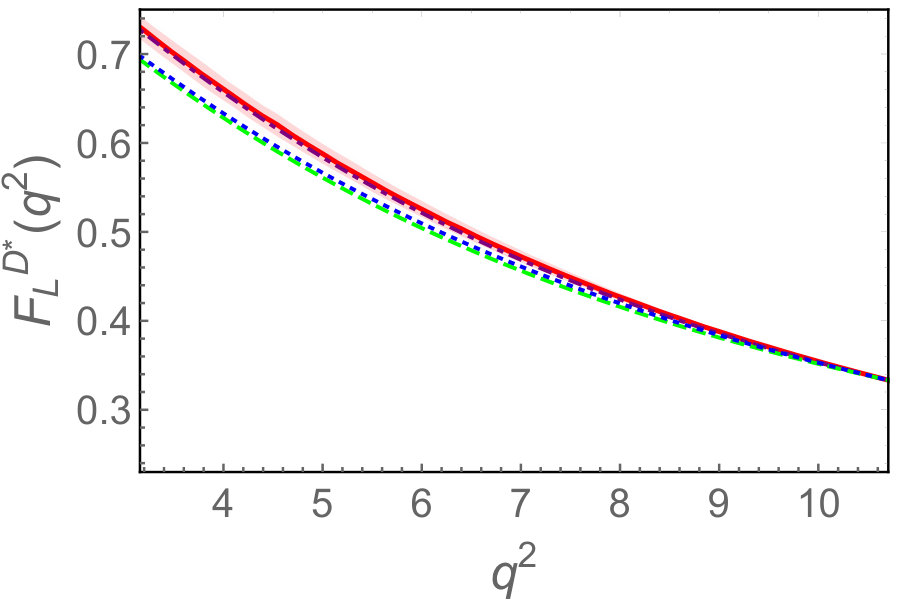 Figure 8
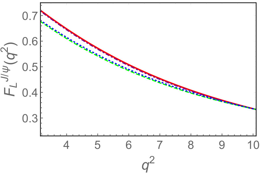 Figure 9
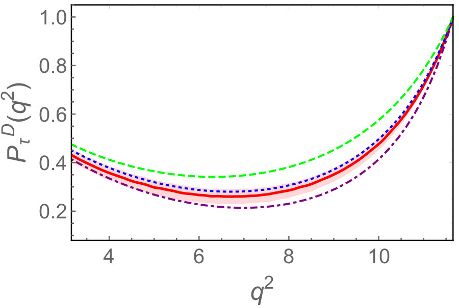 Figure 10
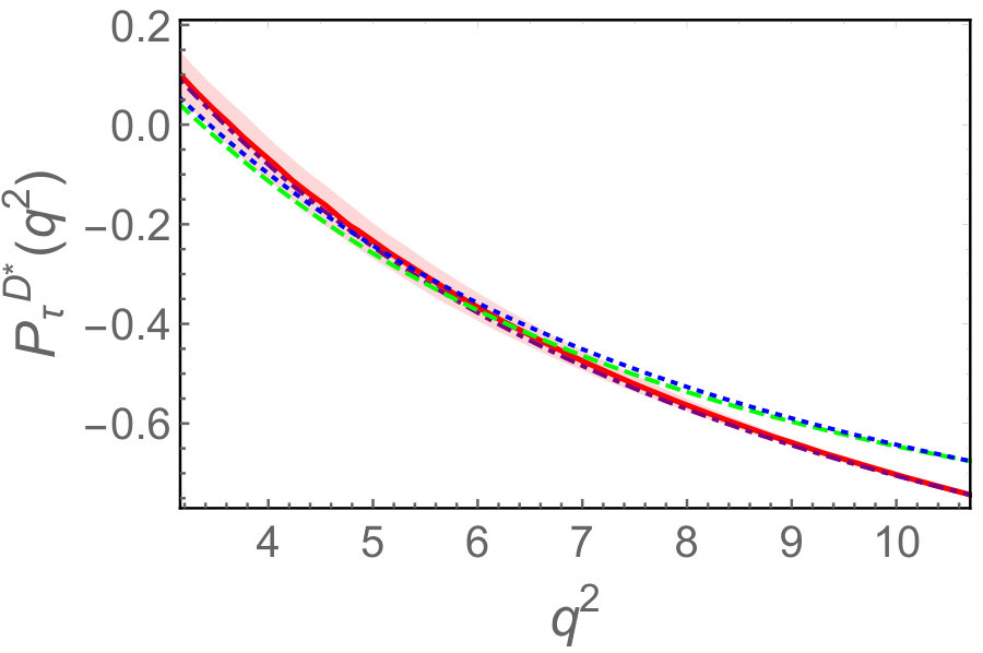 Figure 11
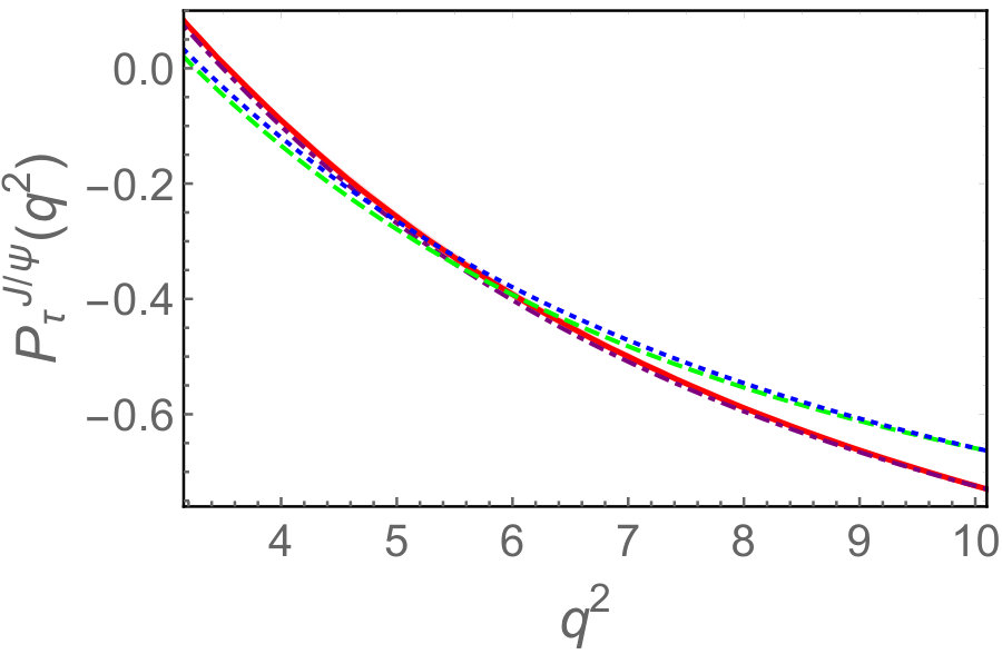 Figure 12
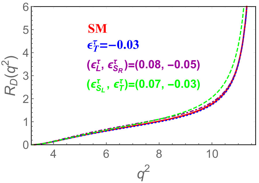 Figure 13
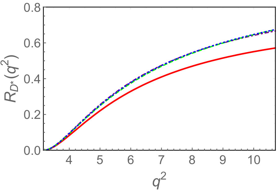 Figure 14
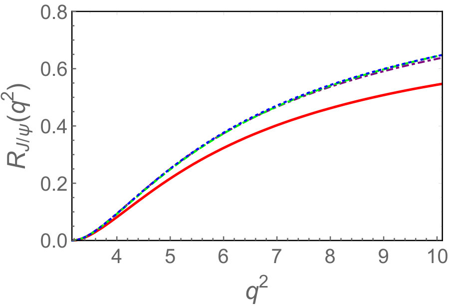 Figure 15
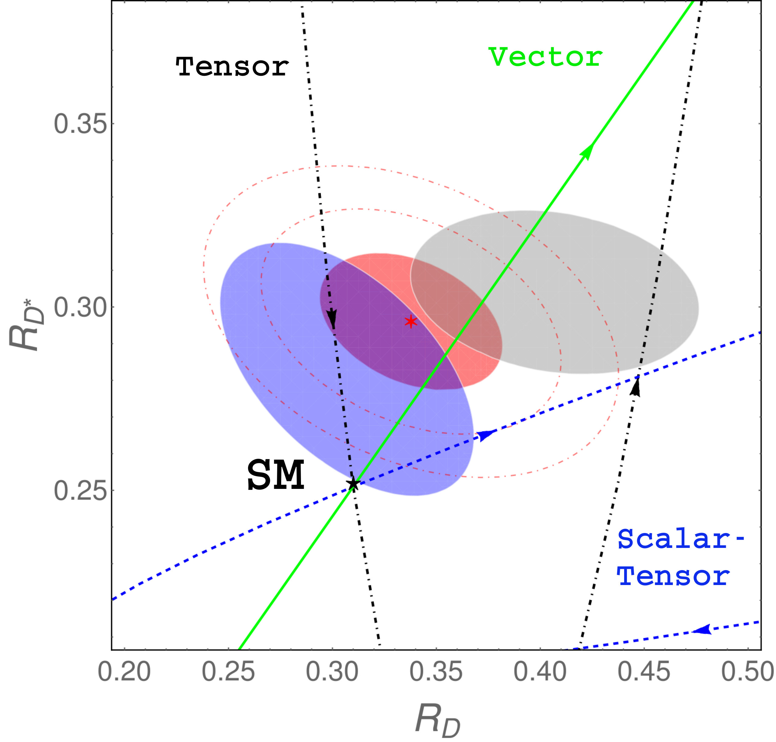 Figure 16
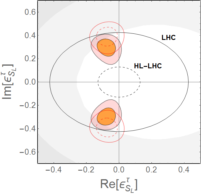 Figure 17
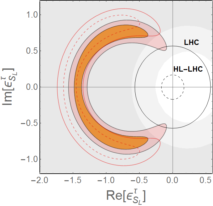 Figure 18
| Observables | Data (averages) | SM | |||
|---|---|---|---|---|---|
| HFLAV 2018 | HFLAV 2019 | ||||
| Mediator | Spin | ||||||||
|---|---|---|---|---|---|---|---|---|---|
| 0 | 1 | 2 | ✗ | ✗ | ✔ | ✔ | ✗ | ||
| 1 | 1 | 3 | 0 | ✔ | ✗ | ✗ | ✗ | ✗ | |
| 1 | 1 | 1 | +1 | ✗ | ✔ | ✗ | ✗ | ✗ | |
| 0 | 1 | +1/3 | ✔ | ✔ | ✗ | ✔ | ✔ | ||
| 0 | 3 | +1/3 | ✔ | ✔ | ✗ | ✗ | ✗ | ||
| 0 | 3 | 2 | +7/6 | ✔ | ✔ | ✗ | ✔ | ✔ | |
| 1 | 3 | 1 | +2/3 | ✔ | ✔ | ✔ | ✗ | ✗ | |
| 1 | 3 | 3 | +2/3 | ✔ | ✔ | ✗ | ✗ | ✗ | |
| 1 | 2 | +5/6 | ✗ | ✗ | ✔ | ✗ | ✗ |
| Best fit | p-value | range | |||
|---|---|---|---|---|---|
| Best fit | p-value | 1 range | |||
|---|---|---|---|---|---|
| Best fit | 1 range | 2 range | 3 range | |
|---|---|---|---|---|
| Observables | SM | ||||
| uncertainty | ||
|---|---|---|
| uncertainty | ||
|---|---|---|
Peer Reviews
No public reviews on file for this paper yet. If you reviewed it on a platform where reviews are public (OpenReview, ICLR, NeurIPS, ICML), you can paste yours below so the community can read it here.
Videos
No videos yet. Explain this paper in a talk, walkthrough, or lecture? Add one.
Revisiting the new-physics interpretation of the data
Rui-Xiang Shi
School of Physics and Nuclear Energy Engineering, Beihang University, Beijing 100191, China
Li-Sheng Geng
School of Physics and Nuclear Energy Engineering & International Research Center for Nuclei and Particles in the Cosmos & Beijing Key Laboratory of Advanced Nuclear Materials and Physics, Beihang University, Beijing 100191, China
Benjamín Grinstein
Department of Physics, University of California, San Diego, 9500 Gilman Drive, La Jolla, CA 92093-0319, USA
Sebastian Jäger
Department of Physics and Astronomy, University of Sussex, Brighton BN1 9QH, United Kingdom
Jorge Martin Camalich
Instituto de Astrofísica de Canarias, C/ Vía Láctea, s/n E38205 - La Laguna, Tenerife, Spain
Universidad de La Laguna, Departamento de Astrofísica, La Laguna, Tenerife, Spain
Abstract
We revisit the status of the new-physics interpretations of the anomalies in semileptonic decays in light of the new data reported by Belle on the lepton-universality ratios using the semileptonic tag and on the longitudinal polarization of the in , . The preferred solutions involve new left-handed currents or tensor contributions. Interpretations with pure right-handed currents are disfavored by the LHC data, while pure scalar models are disfavored by the upper limits derived either from the LHC or from the lifetime. The observable also gives an important constraint leading to the exclusion of large regions of parameter space. Finally, we investigate the sensitivity of different observables to the various scenarios and conclude that a measurement of the tau polarization in the decay mode would effectively discriminate among them.
I Introduction
For some time now, the ratios of semileptonic -decay rates,
[TABLE]
have appeared to be enhanced with respect to the Standard Model (SM) predictions with a global significance above the evidence threshold Lees et al. (2012, 2013); Huschle et al. (2015); Sato et al. (2016); Aaij et al. (2015); Hirose et al. (2017, 2018); Aaij et al. (2018a, b, c); Aoki et al. (2017). In addition, LHCb reports a value of the ratio
[TABLE]
about above the SM Aaij et al. (2018c).
In the SM, semileptonic decays proceed via the tree-level exchange of a boson, preserving lepton universality. Hence, a putative NP contribution explaining the data must involve new interactions violating lepton universality. This may entail the tree-level exchange of new colorless vector () Megias et al. (2017); He and Valencia (2018); Matsuzaki et al. (2017); Babu et al. (2019); Greljo et al. (2018); Asadi et al. (2018) or scalar (Higgs) Tanaka (1995); Celis et al. (2013, 2017); Iguro and Tobe (2017); Fraser et al. (2018); Martinez et al. (2018) particles, or leptoquarks Sakaki et al. (2013); Alonso et al. (2015); Barbieri et al. (2016); Freytsis et al. (2015); Fajfer and Košnik (2016); Bauer and Neubert (2016); Li et al. (2016); Barbieri et al. (2017); Bečirević et al. (2016); Crivellin et al. (2017); Cai et al. (2017); Assad et al. (2018); Di Luzio et al. (2017); Bordone et al. (2018a); Altmannshofer et al. (2017); Monteux and Rajaraman (2018); Marzocca (2018); Blanke and Crivellin (2018); Bordone et al. (2018b); Bečirević et al. (2018); Crivellin et al. (2019); Fornal et al. (2019); Angelescu et al. (2018); Baker et al. (2019); Cornella et al. (2019); Popov et al. (2019) with masses accessible to direct searches at the LHC.
Belle has also measured the longitudinal polarization of the () Hirose et al. (2017) and of the () Abdesselam et al. (2019a) in the decay,
[TABLE]
where refers to the helicity of the particle . While is reconstructed from the hadronic decays of the and is still statistically limited, the reported measurement of is rather precise and disagrees with the SM prediction with a significance of .
Recently, Belle announced a new combined measurement of both and using semileptonic decays for tagging the meson in the event Abdesselam et al. (2019b). This presents a significant addition to the the data set because the previous combined measurements of had been performed at the factories using a hadronic tag. The new result is more consistent with the SM than the previous HFLAV average. Thus, these new data call for a reassessment of the significance of the tension of the signal with the SM and of the possible NP scenarios aiming at explaining it. The purpose of this work is to provide such an analysis using effective field theory (EFT) Buttazzo et al. (2017); Alok et al. (2018a); Azatov et al. (2018a); Bhattacharya et al. (2019); Huang et al. (2018); Asadi et al. (2019); Blanke et al. (2019a); Dutta and Bhol (2017); Dutta et al. (2013); Hu et al. (2019); Alok et al. (2017, 2018b) and to relate it to (partial) UV completions in terms of simplified mediators. We assume that the lepton non-universal contribution affects only the couplings to the tau leptons. A comprehensive analysis of bounds on NP affecting transitions can be found in ref. Jung and Straub (2019). A summary of the recent data (averages) is shown in Table 1, which is compared to the SM predictions which are obtained as specified in Sec. II.3.
II Theoretical framework
II.1 Low-energy effective Lagrangian
The most general effective Lagrangian describing the contributions of heavy NP to semitauonic processes can be written as
[TABLE]
where is the Fermi constant and is the Cabibbo-Kobayashi-Maskawa (CKM) matrix element. The five Wilson coefficients (WCs) , , , and encapsulate the NP contributions, featuring the scaling , where GeV is the electroweak symmetry breaking (EWSB) scale. In the context of the EFT of the SM (SMEFT) Buchmuller and Wyler (1986); Grzadkowski et al. (2010), and the right-handed operator cannot contribute to lepton universality violation at leading order in the expansion Bernard et al. (2006); Cirigliano et al. (2010); Alonso et al. (2015). For this reason, we do not consider the effect of in our fits. Nonetheless, it is important to note that this assumption could be relaxed if there was not a mass gap between the NP and the EWSB scales, or under a nonlinear realization of the electroweak symmetry breaking Catà and Jung (2015).
The chirally-flipping scalar and tensor operators are renormalized by QCD and electroweak corrections González-Alonso et al. (2017); Aebischer et al. (2017); Jenkins et al. (2018); Feruglio et al. (2018). The latter induce a large mixing of the tensor operator into which can have relevant implications for tensor scenarios González-Alonso et al. (2017). As an illustration, defining , (where we have omitted flavor indices), we find that , with González-Alonso et al. (2017)
[TABLE]
and where, in a slight abuse of notation, we keep the notation for the WCs of the low-energy EFT above the EWSB scale. Operators with vector currents do not get renormalized by QCD, whereas electromagnetic and electroweak corrections produce a correction of a few percent to the tree-level contributions Sirlin (1982); González-Alonso et al. (2017). On the other hand, all the operators in the SMEFT matching at low-energies to the Lagrangian in eq. (4) can give, under certain assumptions on the flavor structure of the underlying NP, large contributions to other processes such as decays of electroweak bosons, the lepton and the Higgs, or the anomalous magnetic moment of the muon Feruglio et al. (2017a, b, 2018).
An interesting scenario where the new physics cannot be described by the local effective Lagrangian eq. (4) consists of the addition of new light right-handed neutrinos Bečirević et al. (2016); He and Valencia (2018); Greljo et al. (2018); Asadi et al. (2018); Babu et al. (2019); Robinson et al. (2019); Azatov et al. (2018b). This duplicates the operator basis given in eq. (4) by the replacements in the leptonic currents (and in the hadronic current for the tensor operator) Goldberger (1999); Cirigliano et al. (2010); Robinson et al. (2019) and whose WCs we label with . None of these operators interfere with the SM and their contributions to the decay rates are, thus, quadratic and positive. This also means that the size of the NP contributions needed to explain in this case are larger than with the operators in eq. (4) and they typically enter in conflict with bounds from other processes like the decay Alonso et al. (2017a); Akeroyd and Chen (2017) or from direct searches at the LHC Greljo et al. (2019). As an illustration of the features and challenges faced by these models we consider the operator with right-handed currents,
[TABLE]
(with denoting the right-handed neutrino), which incarnates a popular NP interpretation of the anomaly He and Valencia (2018); Greljo et al. (2018); Asadi et al. (2018); Babu et al. (2019); Robinson et al. (2019); Azatov et al. (2018b). Finally, imaginary parts also contribute quadratically to the rates so we assume the WCs to be real, although we will briefly study also the impact of imaginary parts below.
II.2 Simplified models
The effective operators in eqs. (4), (9) can be mediated at tree level by a number of new particles, that we list in Tab. 2. Possibilities with new charged colorless weak bosons can be realized with the in either a triplet () or a singlet () representation of weak isospin. In the former case, the neutral component of the triplet, a with a mass close to the one of the , produces large effects in either neutral-meson mixing or di-tau production at the LHC, so that this scenario is unavoidably in conflict with data Faroughy et al. (2017). Making the a singlet of weak isospin, =(1, 1,+1) under , requires introducing right-handed neutrinos to contribute to He and Valencia (2018); Greljo et al. (2018); Asadi et al. (2018); Babu et al. (2019); parametrizing the Lagrangian for this model,
[TABLE]
one finds the contribution to the EFT,
[TABLE]
Models based on extending the scalar sector of the SM, such as the two-Higgs doublet model (labeled by in Tab. 2), generate the scalar operators through charged-Higgs exchange. However, these are disfavored by experimental bounds that stem from the lifetime Alonso et al. (2017a) and from the branching fraction of derived using LEP data Akeroyd and Chen (2017). Strong limits from direct searches at the LHC of the corresponding charged scalars have also been obtained in the literature Iguro et al. (2019).
On the other hand, leptoquark exchanges can produce all the operators in eq. (4). 111We follow the notation to label the leptoquark fields introduced in refs. Buchmuller et al. (1987); Doršner et al. (2016). The SM interactions of the scalar leptoquark =(, 1,+1/3) can be described by the Lagrangian,
[TABLE]
where is the antisymmetric tensor of rank two and where we are labeling the flavor of the fields in the interaction basis. This model produces left-handed, scalar-tensor and right-handed contributions Sakaki et al. (2013); Bauer and Neubert (2016); Cai et al. (2017); Crivellin et al. (2017),
[TABLE]
where the coefficients are defined at a scale equal to the leptoquark mass, . The tilde in the coefficients of eq. (13) and in the rest of this subsection indicates that the quark unitary rotations have been absorbed in the definition of the couplings. For instance, if such transformations are , , , , we have defined , and where summation of quark flavor indices is implicit. We have also defined these couplings in the charged-lepton mass basis, ignoring neutrino masses.
The leptoquark with quantum numbers =(3, 2,+7/6) and Lagrangian,
[TABLE]
leads to
[TABLE]
Thus, one can achieve a tensor scenario by adjusting the masses and couplings of the and leptoquarks. It is important to stress that such a solution at low energies requires some tuning due to the large electroweak mixing into scalar operators in eq. (8).
Among the the vector leptoquarks we consider the =(3, 1,+2/3), which has been extensively studied in the interpretation of the anomalies Alonso et al. (2015); Barbieri et al. (2016); Assad et al. (2018); Di Luzio et al. (2017); Bordone et al. (2018a); Monteux and Rajaraman (2018); Marzocca (2018); Blanke and Crivellin (2018); Bordone et al. (2018b); Crivellin et al. (2019); Angelescu et al. (2018); Baker et al. (2019); Cornella et al. (2019),
[TABLE]
leading to left-handed and right-handed contributions, and a scalar contribution,
[TABLE]
In particular, a combination of left-handed and right-handed couplings gives rise to a scalar operator which is instrumental to achieve a better agreement with data in some UV completions of the leptoquark Bordone et al. (2018a, b); Baker et al. (2019); Cornella et al. (2019).
The mediators =(, 3,+1/3) and =(, 3,+2/3) in Tab. 2 provide completions of the left-handed current operator equivalent to the and ones for scalar and vector leptoquark scenarios, respectively. Finally, we have not included in the table the leptoquarks , 2, ) and , 2, ) because they only contribute to scalar and tensor operators with right-handed neutrinos which are not considered in this work, as argued in Sec. II.1.
II.3 Form factors
The hadronic matrix elements in the decay amplitudes are parameterized in terms of the following form factors,
[TABLE]
[TABLE]
[TABLE]
[TABLE]
where , , and stand for vector mesons ( and ) and pseudoscalar mesons ( and ), respectively. We take the quark masses in the scheme, i.e, GeV and GeV Tanabashi et al. (2018),. Note that the -quark mass is derived by the solution of the renormalization group equation for at two-loop order and with three-loop accuracy Buchalla et al. (1996). We follow the PDG Tanabashi et al. (2018) for the masses of the mesons relevant in this work.
For the mode, some of the form factors are taken from Lattice QCD calculations Na et al. (2015); Bailey et al. (2014). The rest are parameterized using heavy-quark effective theory (HQET) Shifman and Voloshin (1988); Isgur and Wise (1989, 1990); Falk et al. (1990); Boyd et al. (1995a, b); Caprini et al. (1998); Fajfer et al. (2012) whose nuisance parameters are determined by the HFLAV global fits to the data Amhis et al. (2014). Our determination of and differs from that of HFLAV in the choice of form factors; ours, based on Ref. Alonso et al. (2016), do not include some recent refinements Bernlochner et al. (2017); Bigi et al. (2017); Jaiswal et al. (2017).
For the form factors, they have been studied in a variety of approaches Wang et al. (2013); Kiselev (2002); Fu et al. (2018); Zhu et al. (2017); Shen et al. (2014); Wang et al. (2009); Hernandez et al. (2006); Ebert et al. (2003); Lytle et al. (2016); Colquhoun et al. (2016); Tran et al. (2018) (for earlier analysis focused on this decay mode see refs. Watanabe (2018); Dutta (2017); Tran et al. (2018); Cohen et al. (2018)). Here we take , , and calculated in the covariant light-front quark model Wang et al. (2009) because these results are well consistent with the lattice results at all available points in Ref. Lytle et al. (2016); Colquhoun et al. (2016). The three tensor form factors can be related through the corresponding HQET form factor at leading order in the heavy-quark expansion,
[TABLE]
with and where we have neglected the power corrections.
II.4 Statistical Method
We follow a frequentist statistical approach to compare the measured values of observables, , to their theoretical predictions as functions of the Wilson coefficients , and of nuisance theoretical parameters . The nuisance parameters parameterize the lack of knowledge (theoretical uncertainties) of the form factors. For the decays, we employ the parametrization and numerical inputs (including correlations) described in ref. Alonso et al. (2016). For the decays we parameterize the theoretical errors reported for the form factors in ref. Wang et al. (2009) as uncorrelated nuisance parameters. We then define a test statistic
[TABLE]
where
[TABLE]
are a set of central values for the nuisance parameters, and and denote the experimental and theoretical covariance matrices, respectively. By adding the theory term we have in effect (from a statistical point of view) added (correlated) “measurements” of the theory parameters to the measurements of the observables.
We will consider scenarios (statistical models) with different subsets of the Wilson coefficients allowed to vary and the remaining ones set to zero, and with various subsets of the experimental observables included. In each case, we obtain best-fit values for the model parameters, including the nuisance parameters, by minimizing . To do so, in a first step we construct a profile- function
[TABLE]
which depends solely on the subset of Wilson coefficients allowed to take nonzero values in a particular scenario, which we again refer to as . (Note that in the case of a single measurement of an observable whose theoretical expression depends linearly on a single theory nuisance parameter , such that is proportional to the theoretical uncertainty, the profiling reproduces the widely employed prescription of combining theoretical and experimental errors in quadrature.) In a second step, we minimize over ; the value(s) of at the minimum provide(s) the best fit (maximum likelihood fit).
Next, we compute a -value to quantify the goodness of fit, i.e. how well a given scenario can describe the data. We will assume that follows a -distribution with degrees of freedom, where is the number of parameters allowed to vary in a given fit. Note that the theory parameters do not contribute to because contains as many “measurements” as theory parameters. In each scenario, the -value is obtained from as one minus the cumulative distribution for degrees of freedom. To illustrate this, let us consider only the including and and ask how well the SM describes these data. For simplicity, let us neglect theory errors altogether (they will be included in the following section, with little impact on the result), taking the SM prediction to be the central values employed by HFLAV2019, and . In this case, there are no parameters to minimize over and is simply a number. This is easily obtained from the HFLAV2019 averages and correlation shown in Table 1, substituting the SM values for the observables, which gives as defined below, and adding a constant as stated by HFLAV 222By adding we are taking into account the goodness of the HFLAV fit to the different measurements of which is needed to obtain an accurate estimate of the -values.. Nine measurements entered the combination and we are determining zero parameters, resulting in . With , this gives a -value of corresponding to , slightly reduced from obtained in an analogous manner from the HFLAV2018 combination.
Finally, for each one-parameter BSM scenario, we construct and obtain confidence intervals from the requirement . Similarly, for each 2-parameter scenario we construct the corresponding and obtain two-dimensional and regions from the conditions and , respectively. We also determine, for each model,
[TABLE]
to quantify at what level the SM point is excluded in that model. The is converted to an equivalent number of standard deviations, referred to as the pull , by employing the cumulative -distribution with set to 1 or 2, the number of jointly determined parameters, as appropriate.
Let us close this section by contrasting to the usual approach for comparing the and measurements to the SM, as employed by HFLAV. In this approach, the true values of and are treated as free parameters, which effectively amounts to a two-parameter BSM model. In this model, HFLAV obtain an SM pull of . We stress that this is a statement about how much better than the SM a BSM model can potentially describe the data. It is conceptually analogous to the pulls in our two-parameter Wilson coefficient fits. (In fact, we will find in the next section a slightly higher pull for two of our 1-parameter models. This comes about because a given value implies a lower -value (higher number of standard deviations) when determining a single parameter as opposed to joint determination of two parameters.) Conversely, our SM -values are a statement how well the SM describes the data, without reference to any comparator BSM model. As we have seen, the data is marginally consistent with the SM at , little changed from 2018. As we will see in the subsequent sections, the impact of the new Belle data on the best-fit values in BSM scenarios is much stronger.
III Results
In this section, we investigate the values of the WCs determined by fitting to the experimental data of , , , and given in Table 1. We also discuss the constraints on scalar operators derived from the limits which are obtained using the lifetime Alonso et al. (2017a) (LEP searches of the decays Akeroyd and Chen (2017)). Note that these limits have been critically discussed in Refs. Blanke et al. (2019a, b); Bardhan and Ghosh (2019). Finally, an upper bound on the values of the WCs can be derived from the tails of the monotau signature (+MET) at the LHC Greljo et al. (2019); Aaboud et al. (2018); Sirunyan et al. (2019) (see below). We will perform fits to two types of dataset: only, as well as to the full dataset in Table 1 including in addition and the polarization observables.
III.1 Fits to only
In Fig. 1 we show the “trajectories” representing the correlated impact on and of NP scenarios where only a single operator is present at a certain scale. Namely, the “vector” curve is followed by scenarios with new pure left-handed () or pure right-handed () currents (which are not affected by short distance QCD corrections). “Tensor” and “scalar-tensor” interpretations involve both and coupled by the radiative corrections in the SM, cf. eq. (8). The tensor trajectory describes a solution with only the tensor operator produced at the heavy scale (cf. produced by the combination of - and -leptoquark contributions described in Sec. II.2), that we take to be 1 TeV. The scalar-tensor description assumes the relation , again, at the heavy scale (cf. produced by the leptoquark). The arrows in the curves signal the direction of positive increment of the WCs. The experimental data in Table 1 is represented by the different ellipses: The gray one is the contour of the 2018 HFLAV average, the blue ellipse is the region of the 2019 Belle measurement with semi-leptonic tag and, finally, the red ellipses are the 1, 2 and 3 contours of the combination of these two.
The interference of the SM with left-handed or scalar-tensor contributions can produce a simultaneous increase of and , as illustrated in Fig. 1 by the positive slope of the corresponding curves at the SM point. This effect drives these solutions to agree well with the 2018 HFLAV average. In case of the tensor scenario, interference with the SM increases at the expense of reducing or vice versa. This effect is illustrated by the negative slope of the “Tensor” curve in Fig. 1. Therefore, the agreement of this scenario with the older data set is due to the quadratic contributions of the tensor operator to the rates. With the new Belle measurement, becomes more consistent with the SM while a value of larger than predicted is still favored. In this new scenario, “vector” models still agree with the data but now the interference of the tensor operator with the SM can play a role in providing a satisfactory solution.
In Table 3 we show the results of fits to all the data on of one or two WCs at a time, while setting the others to zero. In the two-dimensional case we only investigate the interplay between operators with left-handed neutrinos. Setting all WCs to zero, one obtains a . With 9 degrees of freedom (d.o.f) this corresponds to a -value of . As can be inferred from the table, the “vector” operators provide the best one-parameter fit to the data, with a -value of 0.34 and a SM pull of 3.43. The difference in size of the values of the WCs between the left- and right-handed vector solutions is due to the fact that the latter corresponds to a quadratic NP effect in the rates.
The tensor operator also gives a good fit to the data, where the solution driven by the interference piece is now preferred. Scalar models do not provide good fits and require values that may be in conflict with the bounds from . In Fig. 2 we show the functions of the one-parameter fits for each of the WCs. We also show in dashed lines the results obtained from the fits to the 2018 HFLAV average, to emphasize the change in the structure and values of the WCs needed with the new data. Horizontal lines showing the values of the 1- to 4 ranges have been computed taking the best model (vector operators) giving as reference.
In Fig. 3 we show the contour plots that are obtained from each of the six two-dimensional fits to the 2019 HFLAV averages of and . In the Appendix, Table 7, we provide the correlation matrices for the fits to two WCs. We also show with empty red contours the results of the fits to the 2018 HFLAV averages. Black empty contours represent the 2 upper limits that can be set by analyzing the tails of +MET at the LHC (solid line) and by estimating the projected sensitivity at the HL-LHC (dashed line) Greljo et al. (2019).
Adding the new Belle data in the fit results in regions which are slightly closer to the SM, although all NP scenarios still describe the data better with a significance of . As expected, constraints from play an important role in excluding regions of the parameter space of the scalar models. For instance, in case of the pure scalar fit, with , the region is almost excluded by the softer limit based on the lifetime. Even the region is also excluded if the more aggressive limit of 10% on is used. Constraints in the plane are interesting for UV completions involving and leptoquarks. In this scenario, data favors the parameter space in which the two WCs have the opposite sign, like the contribution of the and unlike the one of the , cf. eqs. (13) and eq. (15). A fit with the scalar-tensor contribution produced by the leptoquark (evaluated at TeV) gives a fit with a -value 0.15 that is considerably better than for the SM. However, this scenario performs worse than those with pure left-handed or tensor operators. Constraints in the plane are interesting for UV completions of the leptoquark involving left- and right-handed currents to the fermions Bordone et al. (2018a, b); Baker et al. (2019); Cornella et al. (2019).
The LHC data also probes the parameter space of the preferred regions in the different scenarios. As already anticipated in Greljo et al. (2019), scenarios involving large quadratic contributions of the tensor operator are excluded by more than 2. Furthermore, the current LHC exclusion region independently covers a large portion of the 1 ellipse in the pure scalar scenario and all the parameter space of the region will be probed by the HL-LHC. In fact, with the high-luminosity data set we should be able to probe all the interesting regions in all the scenarios, although less deeply than for the results of the fits to the 2018 HFLAV average.
A potential caveat concerning the interpretation of these LHC bounds is that their validity relies on the assumption that the NP scale is significantly larger than the partonic energies probing the effective interaction in the collisions at the LHC. In ref. Greljo et al. (2019) this was studied by assessing the sensitivity to NP of the distribution in the tau transverse-mass, , of the +MET analyses Aaboud et al. (2018); Sirunyan et al. (2019). Most of the sensitivity of the LHC stems from TeV and, for mediator masses above this mark, the EFT provides a faithful description of the NP signal. By taking the central values of the one-parameter fits shown in Tab. 3, and assuming couplings in eqs. (11), (13), (15) and (17) we find that the masses of the putative new mediators are TeV, TeV for left-handed current couplings and approximately a factor two lighter for right-handed current couplings, cf. TeV. For the tensor scenario, TeV. Therefore, in the comparison with the LHC bounds shown Fig. 3 we are implicitly assuming that the mediators are in this regime of couplings and masses.
Extending the comparison to the right-handed currents, the value obtained in the fit would still be challenged by the bound at resulting from the collider analysis in the EFT. Turning to explicit UV completions in the range of masses below 2 TeV, LHC bounds are stronger than the EFT counterpart for the but weaker for the leptoquarks Greljo et al. (2019) 333For a reanalysis of the impact of the 2019 Belle data in the collider bounds using the monotau searches in the models addressing the anomalies see Talk by J. Martin Camalich, Portorož 2019, Precision era in High Energy Physics (2019).
Finally, in our fits we have assumed real WCs, but is clear from Sec. II.2 that these are generally complex. The imaginary part of WCs does not interfere with the leading, SM contribution. Hence it is expected that fits with purely imaginary WCs are susceptible to bounds from, eg, the rate . This is particularly the case for scalar WCs, that require large magnitude of WCs to account for . For example, in the left panel of Fig. 4 we show the fit of the complex WC with best fit value located at and where the C.L. region is excluded by the lifetime and LHC constraints. However, in some cases allowing a complex phase may improve a WC fit. An interesting example is that of the combination that is the case of the leptoquark mediator, Eq. (15); the right panel of Fig. 4 shows the constraints on the complex plane, with best fit point at , and having imposed the condition at the matching scale .444Complex coefficients for a model based on were considered in Ref. Bečirević et al. (2018).
III.2 Fits to , , , and data
In this section, we perform a global fit of , , and to all the data including and , , and . We implement the LHC monotau constraints by demanding that the WCs are within the corresponding 2 bounds, i.e., we take , , and . In addition, we impose the constraint from the lifetime by requiring that . One obtains a with 12 degrees of freedom (d.o.f) if all the WCs are set to 0, corresponding to a -value of . The resulting WCs from the fit are,
[TABLE]
with the correlation matrix,
[TABLE]
and where for 8 d.o.f., corresponding to a -value of 0.12 and a Pull. This provides an approximation of the in the immediate vicinity of the minimum that is closest to the SM, although it is not appropriate to obtain realistic confidence-level regions. For instance, the intervals may seem to violate the LHC bounds described above.
In order to investigate this in more detail we perform, first, fits of two WCs to and , , and setting the others to 0. This allows one to compare to the results of the two-parameters fits to and presented in Sec III-A. The corresponding six possible combinations of two WCs fits are shown in Fig. 5 and the results of the fits are shown in Table 4. In the Appendix, Table 8, we provide the correlation matrices for these fits. As compared with Fig. 3, one notes that although not precise, the data , and is sensitive enough to exclude the same regions allowed at by the fit to independently excluded by the LHC monotau signature or (see also Ref. Aebischer et al. (2019)). However, for the favored regions of the fits closer to the SM the addition of the current data on these observables has a small impact.
Finally, in order to obtain realistic confidence-level regions with the four active WCs we obtain profile likelihoods functions depending on one or two WCs at a time. The monotau LHC constraints and the lifetime bound are implicitly imposed when profiling over the other ”nuisance” WCs in each case. In Fig. 6, we show the results of the fits as constraints in the six two-WCs plots. In Tab. 5 we show the final , and confidence-level intervals for the WCs. The intervals are consistent with those obtained from the fit in eq. 31, while the and intervals differ from those obtained using the gaussian approximation of the .
III.3 The sensitivity of observables to New Physics
As shown above, different NP scenarios currently give a good description of the data, so the natural question is which other observables, beyond and , allow one to discriminate among them. Only total rates are sensitive to the effects from the vector operators as their effects cancel in normalized observables. On the other hand, scalar and tensor operators change the kinematic distributions of the decays and show up in observables such as tau and recoiling-hadron polarizations (if the latter carries spin), -distribution of the rate or angular analyses.
In Fig. 7, we study the spectra of and of a selection of polarization and angular observables 555 All of them have been defined in Sec. I, except the tauonic forward-backward asymmetry,
(37)
which is independent of overall normalization Alonso et al. (2017b). showing their sensitivity to NP. We select scenarios that can be motivated by UV completions such as those involving scalar-tensor or vector-scalar combinations of operators, and we also study the tensor scenario. The values of the WCs are fixed to the results of the fits to the data, i.e, , , . In Tab 6 we show the results of these observables integrated over the whole kinematic region for the SM and the different NP scenarios considered. Interestingly, none of the preferred scenarios with up to two WCs can satisfactorily describe the Belle measurement of along with the experimental enhancements reported in and .
From the plots in Fig. 7 and predictions in Tab 6, one concludes that a clear pattern emerges in these observables for the different NP scenarios currently favored by the data, although high precision measurements will be required to discriminate among them. The most sensitive ones for this purpose turn out to be the tau polarization and forward-backward asymmetry of the decay mode. Interestingly, with the 50 ab*-1* expected to be collected by Belle II a relative statistical uncertainty better than has been estimated for these observables integrated over the whole region Alonso et al. (2017b).
IV Summary and outlook
In this work, we have studied in detail the status of the new-physics interpretations of the anomalies after the addition of the Belle measurements of using the semileptonic tag and to the data set. We perform two types of fits: First, we fit with one and two parameters (Wilson coefficients) to the 2019 HFLAV average of and with particular attention to the evolution of the preferred scenarios with the new data and to the consistency with the upper bounds that can be derived from the lifetime of the meson and the +MET signature at the LHC. The main conclusion is that NP interpretations driven by left-handed currents and tensor operators are favored by the data with a significance of with respect to the SM hypothesis. Solutions based on pure right-handed currents remain disfavored by the LHC data while scenarios with that only have scalar contributions are in conflict with both, the LHC and the -meson experimental inputs. In fact, the LHC upper bounds currently exclude large regions of the parameter space allowed by the data, and in the high-luminosity phase it should start probing all the interesting regions.
We also perform a second global fit of all the NP operators with (left-handed neutrinos) to the data, , and . The main effect of the added observables, in particular of , is to exclude the regions involving large values of the WCs, in complementarity with the upper LHC bounds. Otherwise, the favored regions by the global fits are equivalent to the ones resulting from the fit to .
A caveat to our conclusions is that the LHC bounds derived from the analysis in terms of effective operators are not applicable if the mass scale of the new mediators they correspond to is lighter than TeV. Scenarios based on and leptoquarks coupled to right-handed neutrinos remain challenged by the monotau signature at the LHC except for the mass range which is being independently probed by pair-production at the LHC. A leptoquark producing a scalar-tensor scenario does not provide a solution as optimal as with the 2018 HFLAV average, whereas in combination with the leptoquark it can provide the optimal tensor scenario. The leptoquark alone can also explain the data successfully when the couplings take complex values and, interestingly, its detection should be at reach in the HL-LHC. Best solutions are incarnated by the and leptoquarks with pure left-handed couplings, possibly in combination with right-hand currents in the latter case.
Finally, we investigate the sensitivity of different observables to NP. We find that the tau polarization in the decay is sensitive to the various scenarios favored by the data. Interestingly, Belle II could achieve a precision in this observable that would provide discriminating power among them.
V Acknowledgments
This work is partly supported by the National Natural Science Foundation of China under Grant No. 11735003 and by the fundamental Research Funds for the Central Universities. BG was supported in part by the US Department of Energy grant No. DE-SC0009919. SJ was supported in part by UK STFC Consolidated Grant ST/P000819/1. JMC acknowledges support from the Spanish MINECO through the “Ramón y Cajal” program RYC-2016-20672.
Note added:
While this paper was being finished different analyses of the new data set of have been reported Murgui et al. (2019); Bardhan and Ghosh (2019); Asadi and Shih (2019).
VI Appendix
In Tables 7 and 8 we provide the correlation matrices for the two-parameter fits to the 2019 HFLAV average of and , Table 3, and to all the observables, Table 4.
The reference list from the paper itself. Each links out to its DOI / PubMed record.
- 1Lees et al. (2012) J. P. Lees et al. (Ba Bar), Phys. Rev. Lett. 109 , 101802 (2012) , ar Xiv:1205.5442 [hep-ex] . · doi ↗
- 2Lees et al. (2013) J. P. Lees et al. (Ba Bar), Phys. Rev. D 88 , 072012 (2013) , ar Xiv:1303.0571 [hep-ex] . · doi ↗
- 3Huschle et al. (2015) M. Huschle et al. (Belle), Phys. Rev. D 92 , 072014 (2015) , ar Xiv:1507.03233 [hep-ex] . · doi ↗
- 4Sato et al. (2016) Y. Sato et al. (Belle), Phys. Rev. D 94 , 072007 (2016) , ar Xiv:1607.07923 [hep-ex] . · doi ↗
- 5Aaij et al. (2015) R. Aaij et al. (LH Cb), Phys. Rev. Lett. 115 , 111803 (2015) , [Addendum: Phys. Rev. Lett.115,no.15,159901(2015)], ar Xiv:1506.08614 [hep-ex] . · doi ↗
- 6Hirose et al. (2017) S. Hirose et al. (Belle), Phys. Rev. Lett. 118 , 211801 (2017) , ar Xiv:1612.00529 [hep-ex] . · doi ↗
- 7Hirose et al. (2018) S. Hirose et al. (Belle), Phys. Rev. D 97 , 012004 (2018) , ar Xiv:1709.00129 [hep-ex] . · doi ↗
- 8Aaij et al. (2018 a) R. Aaij et al. (LH Cb), Phys. Rev. Lett. 120 , 171802 (2018 a) , ar Xiv:1708.08856 [hep-ex] . · doi ↗