Equilibration on average in quantum processes with finite temporal resolution
Pedro Figueroa-Romero, Kavan Modi, Felix A. Pollock

TL;DR
This paper investigates when multi-time quantum processes with limited temporal resolution can be approximated by equilibrium processes, extending the concept of equilibration on average to multiple times and providing bounds on distinguishability.
Contribution
It generalizes the notion of equilibration on average to multi-time processes with finite temporal resolution and establishes bounds on their distinguishability from equilibrium.
Findings
Derived conditions for multi-time equilibration with finite temporal resolution
Established an upper bound on a distinguishability measure between processes
Identified multi-time contributions depending on temporal resolution and observer disturbance
Abstract
We characterize the conditions under which a multi-time quantum process with a finite temporal resolution can be approximately described by an equilibrium one. By providing a generalization of the notion of equilibration on average, where a system remains closed to a fixed equilibrium for most times, to one which can be operationally assessed at multiple times, we place an upper-bound on a new observable distinguishability measure comparing a multi-time process with a finite temporal resolution against a fixed equilibrium one. While the same conditions on single-time equilibration, such as a large occupation of energy levels in the initial state remain necessary, we obtain genuine multi-time contributions depending on the temporal resolution of the process and the amount of disturbance of the observer's operations on it.
Click any figure to enlarge with its caption.
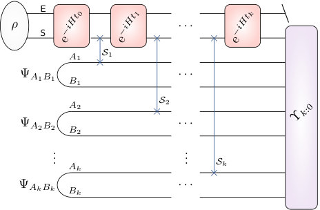 Figure 1
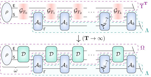 Figure 1
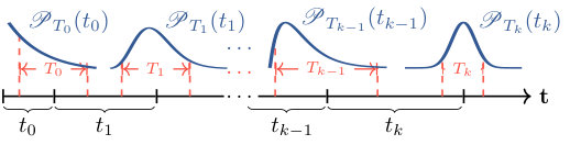 Figure 2
Peer Reviews
No public reviews on file for this paper yet. If you reviewed it on a platform where reviews are public (OpenReview, ICLR, NeurIPS, ICML), you can paste yours below so the community can read it here.
Videos
No videos yet. Explain this paper in a talk, walkthrough, or lecture? Add one.
Equilibration on average in quantum processes with finite temporal resolution
Pedro Figueroa–Romero
Kavan Modi
Felix A. Pollock
School of Physics & Astronomy, Monash University, Victoria 3800, Australia
Abstract
We characterize the conditions under which a multi-time quantum process with a finite temporal resolution can be approximately described by an equilibrium one. By providing a generalization of the notion of equilibration on average, where a system remains closed to a fixed equilibrium for most times, to one which can be operationally assessed at multiple times, we place an upper-bound on a new observable distinguishability measure comparing a multi-time process with a finite temporal resolution against a fixed equilibrium one. While the same conditions on single-time equilibration, such as a large occupation of energy levels in the initial state remain necessary, we obtain genuine multi-time contributions depending on the temporal resolution of the process and the amount of disturbance of the observer’s operations on it.
Suggested keywords
A fundamental question at the core of statistical mechanics is that of how equilibrium arises from purely quantum mechanical laws in closed systems. This phenomenon is generically known as equilibration or thermalization, where in the latter case the system relaxes to a thermal state. The dissipative nature of equilibration, however, is at odds with the unitary nature of quantum mechanics. There are three main approaches to resolving this conundrum: typicality Popescu et al. (2006); Gogolin (2010); Gemmer et al. (2009); Goldstein et al. (2010); Gogolin and Eisert (2016); Garnerone (2013), which argues that small subsystems of a composite are in thermal equilibrium for almost all pure states of the whole; dynamical equilibration on average Tasaki (1998); Reimann (2008); Linden et al. (2009); Short (2011); Short and Farrelly (2012); Wilming et al. (2018), which demonstrates that time-dependent quantities of quantum systems evolve towards fixed values and stay close to them for most times, even if they eventually deviate greatly from it; and the eigenstate thermalization hypothesis Deutsch (1991); Srednicki (1994, 1999); Steinigeweg et al. (2013); Rigol et al. (2008); Turner et al. (2018), which argues that the expectation values of a ‘physical observable’ at long times are indistinguishable for an isolated system from a thermal one.
What these approaches have in common, is that they look at the statistical properties of the state of the system at long times; however, finding a system in or close to an equilibrium state does not necessarily imply all observable properties of the system have equilibrated. In particular, when measurements are coarse (i.e. only a subpart is measured), it may be that temporal correlations due to a sequence of observations may contain signatures indicating whether the system is in equilibrium or not. The recent studies of out-of-time-order correlation functions use multi-time statistics to distinguish between thermalised systems and coherent complex systems Alexei Kitaev (2014). However, it may be that these multi-time statistics also equilibrate in general; that is, they are most often found close to some average value.111The out-of-time-order correlations require propagating the system back and forth in time. Here we only go forward in time.
In this manuscript, we focus on the case of finite temporal resolution for the dynamical equilibration of quantum processes where multiple operations are applied in sequence. We present sufficient conditions for general multi-time observations to relax close to their equilibrium values when the corresponding operations are implemented with an imperfect, or fuzzy, clock (or, equivalently, on a system with uniformly fluctuating energies). In particular, we place an upper bound on how distinguishable the statistics of such observations are from those made in equilibrium.
We first briefly recapitulate the landmark results of Refs. Short and Farrelly (2012); Reimann (2008), in which the attainability of observable equilibration on average for a single observation is characterized mainly by two factors: the energy eigenstates of the system having a large overlap with the initial state, and the scale set by the operator norm of the observable being measured. Building on the works of Refs. Short and Farrelly (2012); Reimann (2008), we first ask, for the case of a single measurement, how different is an equilibrium process from an out-of-equilibrium one, when the available clock is fuzzy. We then generalise to considering observations over multiple points in time; here, temporal correlations become relevant. While the original conditions for equilibration to occur still hold, we obtain additional conditions related to the temporal resolution of the observations and how much these disturb the intermediate states. Our results hold for Hamiltonian dynamics of the total system, while the measurements are allowed to be general quantum operations that are coarse and may only act on a sub-part of the whole system.
I Equilibration on average
In the past decade, the program of equilibration has focused on upper bounding fluctuations of observable expectation values around equilibrium, from which conclusions about equilibration of the state of the system itself have been drawn Short (2011); Gogolin and Eisert (2016). The basic mechanism behind equilibration is that of dephasing Reimann (2008); de Oliveira et al. (2018), and equilibration will occur as long as the initial state, following a perturbation, has an overlap with many energy eigenstates of the Hamiltonian driving the dynamics. The only further assumption is that there are not too many degenerate energy gaps Gallego et al. (2018), ensuring that the majority of the system plays a dynamical role Linden et al. (2009). Specifically, observable equilibration in the sense of Ref. Short and Farrelly (2012) considers time-independent Hamiltonian dynamics given by a unitary operator , with results depending on energetic properties of the Hamiltonian , such as the number of distinct energy levels and the maximum number of energy gaps in an energy window of width .
While the choice of an equilibrium state is arbitrary, an intuitive candidate is the infinite-time-averaged subsystem state
[TABLE]
where stands for the initial state of the whole system, time-averaged over a finite time window of width . Notably, this corresponds to a dephasing of the initial state with respect to , i.e. where we define
[TABLE]
with a projector onto the th eigenspace of . In fact, we can similarly describe general finite-time-averaged evolution by the map
[TABLE]
Whenever it is clear that the averaging window is , we will simply denote these by and .
In this minimal setting, the authors of Ref. Short and Farrelly (2012) prove an important result on observable equilibration by showing the closeness between the evolved state and . Specifically, they upper-bound the temporal fluctuations of the expectation value of a general operator around equilibrium within a finite-time window as
[TABLE]
where and denotes largest singular value; crucially, the so-called inverse effective dimension (or inverse participation ratio) of the initial state, , quantifies the number of energy levels contributing significantly to the dynamics of the initial state .
In general, we have the hierarchy , and this result implies that equilibration is attained for large . It has been argued, on physical grounds, that the effective dimension takes a large value in realistic situations Gogolin and Eisert (2016); Reimann (2008), increasing exponentially in the number of constituents of generic many-body systems Wilming et al. (2018), and it has been proven that it takes a large value for local Hamiltonian systems whenever correlations in the initial state decay rapidly Farrelly et al. (2017). The temporal fluctuations of the expectation values of around equilibrium constitute a meaningful quantifier of equilibration: a small variance relates to the expectation value of concentrating around its mean 222Strictly, the full statistics should then display equilibration..
This behaviour of long-time fluctuations around equilibrium has been studied both analytically and numerically in various physical models Ziraldo et al. (2012); Venuti and Zanardi (2013); Zangara et al. (2013); Campos Venuti and Zanardi (2014); Schiulaz et al. (2020), as well as for the more restrictive case of thermalization Rigol et al. (2008); Mori et al. (2018); Gluza et al. (2019); Wilming et al. (2019). Similarly, related questions such as an absence of equilibration Basko et al. (2007); Nandkishore and Huse (2015); Hess et al. (2017); Hamazaki and Ueda (2018), or the robustness of equilibration and further relaxation after a perturbation have been investigated Robinson (1973); Kiendl and Marquardt (2017); Farrelly et al. (2017); Gallego et al. (2018); Knipschild and Gemmer (2018). Here, we take a related approach towards investigating the behaviour of quantum quantum process when the interrogations are fuzzy in time. Doing so gives focus on an operationally meaningful scenario where we show that observations that have a finite temporal resolution make it hard to tell an out-of-equilibrium process from one that is in equilibrium.
II Equilibration due to finite temporal resolution
Motivated by the above result, we consider the operationally relevant implications of limited resolution in time. Firstly, we focus on the dynamics of a -dimensional subpart of a -dimensional system , and we refer to subsystem equilibration as the relaxation of towards some steady state, while the whole evolves unitarily with a general time-independent Hamiltonian ; our results can then naturally reduce to closed-system equilibration if coarse operations on the whole are considered. We then ask how different an evolving quantum state appears from equilibrium when measured at a time that can vary in each realisation, being randomly drawn from some distribution that quantifies the fuzziness associated with finite temporal resolution.
Specifically, by a finite-temporal resolution observation we mean an observable (either on subsystem or acting coarsely on ) measured after a time sampled from a probability distribution with density function , i.e. which is such that . Here the parameter represents the uncertainty or fuzziness of the distribution; for example, it could be associated with the variance of the distribution. With this definition, we may generalize the time-average over a time-window by
[TABLE]
In particular, we require that the distributions are such that the finite-time averaging map gives the dephasing map in the infinite-time limit, , or equivalently, such that ; this also renders the equilibrium state to be independent of the particular choice of distribution.
The average distinguishability by means of an observable between the equilibrium and non-equilibrium cases can be quantified as . This can be upper-bounded by
[TABLE]
where and . Here and is the difference in purity of the full state with respect to that of the equilibrium .
Proof. Given that and , Eq. (6) follows because
[TABLE]
where we used , as .
In general , with equality both for pure or when the Hamiltonian is non-degenerate; both quantities relate to how spread the initial state is in the energy eigenbasis.
In particular, when the fuzziness corresponds to that of the uniform distribution over an interval , the probability density function is , as in the results of Ref. Short and Farrelly (2012) outlined above, and we get with . The bound in Eq. (6) then tells us that the evolved state will differ from the equilibrium when measured at a given time with a temporal-resolution at most with proportion for the smallest energy gap , with a scale set by the size of the observable and how different the initial state is from the equilibrium .
One, however, might not stop at a single observation but continue gathering data to assess how close the system remains to equilibrium with respect to a set of possible operations, , as we suggestively depict in Fig. 1. The reason for fuzziness in the initial time is that we do not know when the process actually began. However, one question we can ask is whether, by making a sequence of measurements, we are able to overcome the fuzziness of the initial interval. These operations can correspond to any possible experimental intervention, which can be correlated with any other interventions previously made, through an ancillary system. In this case the information between time-steps propagated through the environment and the disturbance introduced by the operations might become relevant. However, the subsequent measurements will also suffer from some level of fuzziness and this must be accounted for. We now precisely establish the description for multi-time quantum processes in such generality, followed by a generalisation of Eq. (6) through an upper bound to the distinguishability between a finite-time resolution process and an equilibrium one.
III Multi-time quantum processes
Consider an initial state of the joint system unitarily evolving through a time-independent Hamiltonian dynamics until, at time , an operation is made on along with an ancilla , which is initially uncorrelated in state . We denote the full initial state by . After the first operation, the environment and system evolve unitarily again for a time until another operation is made on , and so on for time-steps. The joint expectation value of the series of operations is given by
[TABLE]
where acts on , while by an operation we explicitly mean , with , which acts solely on ; here are Kraus operators, potentially corresponding to measurement outcomes, and are the corresponding outcome weights. The Hamiltonians are in general different at each step. The ancillary space can be interpreted as a quantum memory device, and might carry information about previous interactions with the system.
The information about the intrinsic dynamical process, i.e., the initial state and the joint unitary evolutions with their respective timescales at each step, can be encoded in a positive semi-definite tensor , and similarly, the sequence of operations can be encoded in a tensor of the form , as depicted in Figure 1 and detailed in Appendix A. This simplifies the joint expectation value in Eq. (8) as the inner product
[TABLE]
which can be seen as a generalisation of the Born rule to multi-time step quantum processes Costa and Shrapnel (2016). Here, becomes an unnormalized many-body density operator, and an observable. Temporal correlations, or memory, in operations are carried through space ; any can be represented as a sequence of uncorrelated operations on a joint system. Both classically correlated operations, where the measurement basis is conditioned on past outcomes, and coherent quantum correlated measurements can be represented in this way Taranto et al. (2019a). The case of infinite memory and the case of completely uncorrelated operations are then extreme limits of this general setting. Formally, is the Choi state Watrous (2018) of a quantum process, containing all its accessible dynamical information Taranto et al. (2019b, a) and is the quantum generalisation of a stochastic process Milz et al. (2020); Pollock et al. (2018a, b); Milz et al. (2017).
We finally notice that when a process ends at the first intervention we have , becoming the corresponding quantum state, so that all of the previous results (single measurement) apply for such case.
IV Equilibration of multi-time observables
Consider a quantum process as above with a fixed single Hamiltonian for all time intervals such that . In Appendix B we present the general case where we do not make this assumption. This multi-time process consists of free evolution sandwiched by generalised measurements. We denote the time intervals of the free evolutions as , which is preceded by the -th measurement and followed by -th measurement. In other words, is the waiting time between -th and -th measurements. As before, each of these waiting times is allowed to be fuzzy, taking a value sampled from probability distribution , i.e. . We denote the average length as
[TABLE]
We pictorially represent this in Fig. 2. We denote multi-time probability distribution as , where
[TABLE]
are waiting times and the fuzziness parameters for each time interval, respectively; in what follows, we take for simplicity (see Appendix B for the general case). The corresponding finite-temporal-resolution process is then given by
[TABLE]
We are interested in quantifying how different this out-of-equilibrium process, where time intervals are fuzzy, looks from an equilibrium process. To define the equilibrium process we follow the lead of earlier results, i.e., the initial state relaxes to the equilibrium state until an operation is made, and subsequently the system relaxes again to an equilibrium state until an operation is made, and so on for -time-steps. This then leads to the definition
[TABLE]
as the equilibrium states after each intervention up to . This is a sensible definition for the intermediate equilibrium states, which, however, is dependent on each operation . We can now define the equilibrium quantum process as
[TABLE]
This is depicted in Fig. 1 as a set of dephasing maps at each timestep. This means then that we can write for the expectation of a sequence of operations on the equilibrium process , where equivalently, . Since we can also express each finite averaging in the energy eigenbasis using the partial dephasing map , defined in Eq. (3), we can similarly write , where we now define
[TABLE]
as intermediate, finite-time-averaged states after each intervention up to . As by definition , the infinite-time limits make indistinguishable from . We also depict this in Fig. 1.
We may then generalize the left hand side in Eq. (6) to general quantum processes with , asking how different the statistics of a set of operations can be on a fuzzy clock process, , as opposed to those in the equilibrium one . We provide one such answer with the following,
Theorem**.**
Given an environment-system-ancilla with initial state and initial equilibrium state , for any -step process with an evolution generated by a time-independent Hamiltonian on , and for any fuzzy multi-time observable corresponding to a sequence of temporally local operations each with fuzziness acting on a joint system,
[TABLE]
where here and is a composition of operations; the norm here stands for the norm on superoperators induced by the Frobenius norm, ; the first is a single-time equilibration contribution, whereas the second term contains multi-time contributions where
[TABLE]
with and intermediate finite-time averaged and equilibrium states at step and where denotes a commutator of superoperators.
The proof is given in full in Appendix B.
In general, by definition the term , which depends on the waiting time distribution , converges to zero in increasing , with the rate of convergence depending on the specific distribution. In particular, for the uniform distribution on all time-steps, as in the approach by Short and Farrelly (2012), we average over a time-window of width around each for all time-steps, with in the interval , and outside it. This yields ; the term then picks the smallest non-zero energy gap in the Hamiltonian. Similarly, if the fuzziness corresponds to that of a half-normal distribution with variance , then overall decays exponentially with
[TABLE]
where is the error function and . For both cases, if is small, will also be vanishingly small whenever the energy gap that maximizes is large enough, i.e. . This property holds in general, since distributions can be approximated as uniform for small or because the gaps can be seen as a rescaling factor on in the definition of .
The term in Eq. (17) neglects temporal correlations and the operations are all composed as a single operation . The two-norm distance satisfies as the ancillary input can be taken to be pure. As discussed above, this term is suppressed through the contributions when the averaging window, or equivalently the fuzziness of the clock is large enough and for small whenever the energy gap maximizing the time-averaging factor is large with respect to .
The second term in Eq. (16) contains genuine multi-time contributions to the bound for equilibration, which we bound further in Appendix B. These terms relate to how well intermediate states, at step , equilibrate. Crucially, we show that the term in Eq. (18) can be upper-bounded as , so that it is suppressed overall in the width of the time-window . For the term in Eq. (19), notice that expanding and using the triangle inequality,
[TABLE]
where each term is the purity of a dephased state, which will decay as the effective dimension of that state.333 In general, for any state , with equality for either pure states or non-degenerate Hamiltonians. On the other hand, when the control operations from [math] to succeed in driving so that the action of the commutator on it does not dephase it so much, the purity of may be large and thus may become trivial (i.e. it approaches 1).
More concretely, the operations interleaved within the intermediate states and will relate in Eq. (18) and Eq. (19) to how greatly they disturb either the finite-time averaged or the equilibrated . This is most evident in the terms , which can be bounded as . The norm of the commutator can be written in terms of both the capacity of the operations to generate coherences between different energy eigenspaces from equilibrium and the degree to which the operations can turn such coherences into populations. Environments in physical systems are typically much larger than the subsystems that can be probed, and, keeping in mind that the operations act only on subsystem and the ancilla , the ability to generate and detect energy coherences should be severely limited in many physically relevant cases.
V Conclusions
We have introduced an extended notion of equilibration that pertains to observations made across multiple times with a finite-temporal resolution. In a similar way to the standard case of equilibration for observables at a single time, we have put bounds on the degree to which it holds that depend on the Hamiltonian driving the evolution. We have shown that either subsystems or global coarse properties of a closed time-independent Hamiltonian system will display equilibration for multiple sequential operations with a temporal uncertainty or fuzziness provided both the initial and intermediate states have a significant overlap with the energy eigenstates, the temporal fuzziness is large enough relative to the average measurement time or, equivalently, the energy gaps in the Hamiltonian are large enough with respect to small temporal fuzziness, and the disturbance by the operations on intermediate states is small.
Our approach for the operations that can act on the process is general in the sense that these are completely positive maps which can be correlated between time-steps and propagate information from their interactions with the subsystem through the ancillary space . While these set a scale in all terms of the right-hand side of Eq. (16), they can also contribute to loosen it, potentially allowing to distinguish the fuzzy process from the equilibrium one within a finite time. It is not entirely clear, however, if a departure from equilibration is more readily accessible with a larger ancillary space and for long time fuzziness the upper-bound in Eq. (16) should remain close to zero.
Similar to the single-time standard case, equilibration over multiple observations is expected intuitively through decoherence arguments Yukalov (2012). The interplay with memory effects, through both the environment and the ancillary space in the interventions is as yet not entirely clear, e.g., under which circumstances finite-temporal resolution equilibration can occur without the dynamics being Markovian, i.e., memoryless, or if the temporal correlations among interventions through the ancillary space can display a departure from equilibration within a finite-time. We have previously shown rigorously that most processes in large dimensional environments are close to Markovian, and hence strongly equilibrate, in the strong coupling limit in a full typicality sense Figueroa-Romero et al. (2019), as well as on complex systems obeying a large deviation bound Figueroa-Romero et al. (2020), but outside this regime the relationship between the two properties is less transparent.
Acknowledgements.
We are grateful to Daniel Burgarth and Lucas Céleri for valuable discussions. PFR is supported by the Monash Graduate Scholarship (MGS) and the Monash International Postgraduate Research Scholarship (MIPRS). KM is supported through Australian Research Council Future Fellowship FT160100073.
Appendix A The process tensor
The process tensor is defined as a linear, completely positive (CP) and trace non-increasing map from a set of CP maps referred to as control operations, e.g. measurements, to a quantum state, and its action can be described as a multi-time open system evolution, e.g. for joint unitary evolution of an environment plus system , with , a -step process is determined by
[TABLE]
where is an initial joint state, are unitary maps acting on , and the maps act solely on subsystem . We employ weighted operations, i.e. such that where are the Kraus operators of satisfying and are the outcome weights for .
The associated Choi state of a time-evolved process tensor with initial state is then given by
[TABLE]
where is maximally entangled and unnormalized, and where here
[TABLE]
with all identity operators in the total ancillary system and with the being unitary operators at step , and
[TABLE]
with . This can be visualised as the quantum circuit depicted in Figure 3 when the unitary evolution is determined by a time-independent Hamiltonian, as we detail below, and we highlight that is defined directly with the first input being the initial state (as opposed to half of a maximally entangled state in ). Explicitly, it can be written as
[TABLE]
, and . Also notice that the resulting Choi process tensor state belongs to the whole plus ancillary system, which has dimension .
In particular, here we deal with evolution by time-independent Hamiltonians , i.e., with . Also, as done in Short (2011); Short and Farrelly (2012); Linden et al. (2009), we consider first a pure initial state and then extend our results to mixed initial states by purification; this also allows to choose an energy eigenbasis for such that the evolution of the initial state is the same as that given by a non-degenerate Hamiltonian , i.e.,
[TABLE]
where .
Appendix B Proof of the main result
We consider the multi-time expectation for CP (weighted) maps acting on a subsystem of a joint system, together with an ancillary space , where the weights are and with . The full initial -state will be given by , where acts on . This expectation in a process is given by
[TABLE]
where implicitly ’s act only on , while the unitaries with act on the system. We consider a fixed set of projectors for all Hamiltonians such that at each step , with projecting onto the energy eigenspaces of with energy . We also denote simply by the composition of superoperators when clear by context. Let
[TABLE]
for a probability distribution on all with density function with a parameter , and similarly,
[TABLE]
for all . These probability functions are set to be such that
[TABLE]
with the parameters taking the role of an uncertainty parameter, e.g. the variance of a given distribution.
We now define where the overline means time-average over all , i.e.
[TABLE]
In general, we can write
[TABLE]
for any . Let us denote by and the dephasing map with respect to , then we can similarly write
[TABLE]
and so
[TABLE]
We now consider the difference
[TABLE]
where
[TABLE]
with
[TABLE]
Defining , this is . Let us define the partial dephasing superoperator by and , such that . Whenever we denote , this means , and similarly for any other maps.
Let us look first at the case (we label with a subindex the step at which is applied where relevant),
[TABLE]
where the third line follows by the triangle inequality (, here with ). Similarly, for general ,
[TABLE]
where . Using the Schwartz inequality as , where here we denote for simplicity, we further find
[TABLE]
For the first term of Eq. (42), we have , therefore,
[TABLE]
where we used , because . This, together with Eq. (42) already gives the result in Eq. (16) for the case and for all .
For the second term then, similarly,
[TABLE]
as .
For the third term, with ,
[TABLE]
Finally, for the fourth term, as
[TABLE]
then, let us denote , so that putting all together,
[TABLE]
as discussed in the main text.
The reference list from the paper itself. Each links out to its DOI / PubMed record.
- 1Popescu et al. (2006) S. Popescu, A. J. Short, and A. Winter, Nat. Phys. 2 , 754 (2006) . · doi ↗
- 2Gogolin (2010) C. Gogolin, Pure State Quantum Statistical Mechanics , Ph.D. thesis , Julius-Maximilians-Universitat Wuurzburg Theoretische Physik III (2010).
- 3Gemmer et al. (2009) J. Gemmer, M. Michel, and G. Mahler, Quantum Thermodynamics: Emergence of Thermodynamic Behavior Within Composite Quantum Systems , Lecture Notes in Physics (Springer Berlin Heidelberg, 2009).
- 4Goldstein et al. (2010) S. Goldstein, J. L. Lebowitz, C. Mastrodonato, R. Tumulka, and N. Zanghí, P. Roy. Soc. A-Math. Phy. 466 , 3203 (2010) . · doi ↗
- 5Gogolin and Eisert (2016) C. Gogolin and J. Eisert, Rep. Prog. Phys. 79 , 056001 (2016) . · doi ↗
- 6Garnerone (2013) S. Garnerone, Phys. Rev. B 88 , 165140 (2013) . · doi ↗
- 7Tasaki (1998) H. Tasaki, Phys. Rev. Lett. 80 , 1373 (1998) . · doi ↗
- 8Reimann (2008) P. Reimann, Phys. Rev. Lett. 101 , 190403 (2008) . · doi ↗