Sample Paths Estimates for Stochastic Fast-Slow Systems driven by Fractional Brownian Motion
Katharina Eichinger, Christian Kuehn, Alexandra Neamtu

TL;DR
This paper investigates how additive fractional noise with H > 1/2 influences fast-slow systems, providing probabilistic bounds and neighborhood estimates, especially in systems with hyperbolic stable slow manifolds, with applications to climate modeling.
Contribution
It extends sample path estimates to fractional Brownian motion driven systems, overcoming the lack of martingale methods and providing high-probability neighborhoods for such systems.
Findings
High-probability neighborhoods containing the process are established.
Exponential error estimates quantify the probability of system leaving the neighborhood.
Application demonstrated in a climate modeling example with time-correlated noise.
Abstract
We analyze the effect of additive fractional noise with Hurst parameter on fast-slow systems. Our strategy is based on sample paths estimates, similar to the approach by Berglund and Gentz in the Brownian motion case. Yet, the setting of fractional Brownian motion does not allow us to use the martingale methods from fast-slow systems with Brownian motion. We thoroughly investigate the case where the deterministic system permits a uniformly hyperbolic stable slow manifold. In this setting, we provide a neighborhood, tailored to the fast-slow structure of the system, that contains the process with high probability. We prove this assertion by providing exponential error estimates on the probability that the system leaves this neighborhood. We also illustrate our results in an example arising in climate modeling, where time-correlated noise processes have become of greater…
Click any figure to enlarge with its caption.
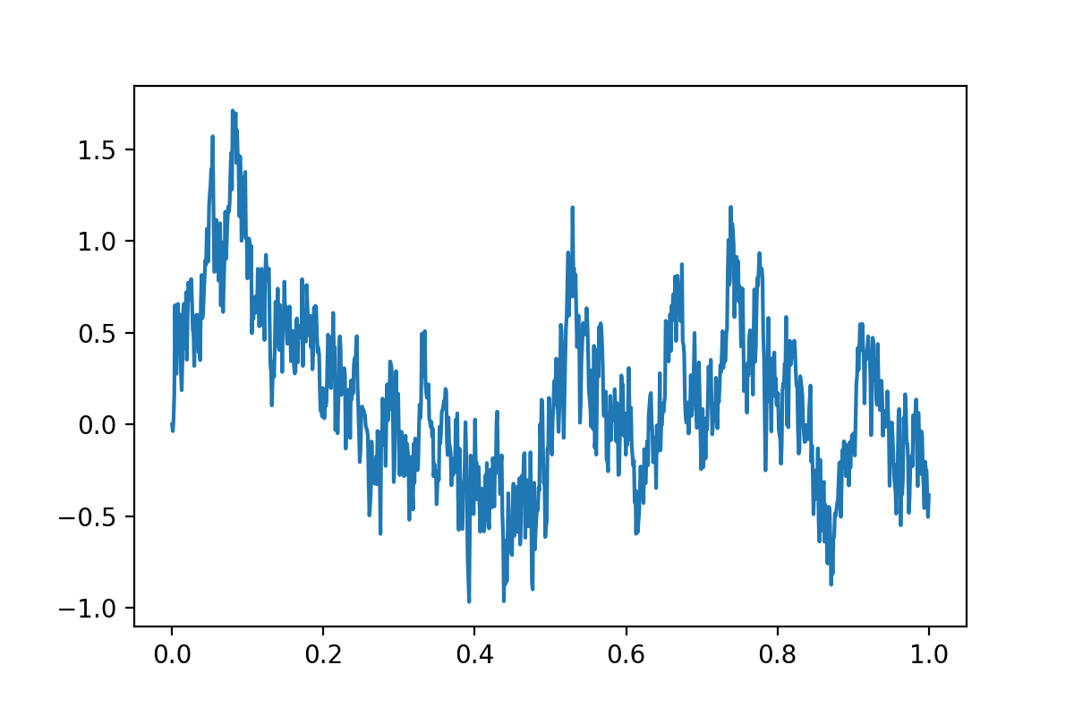 Figure 1
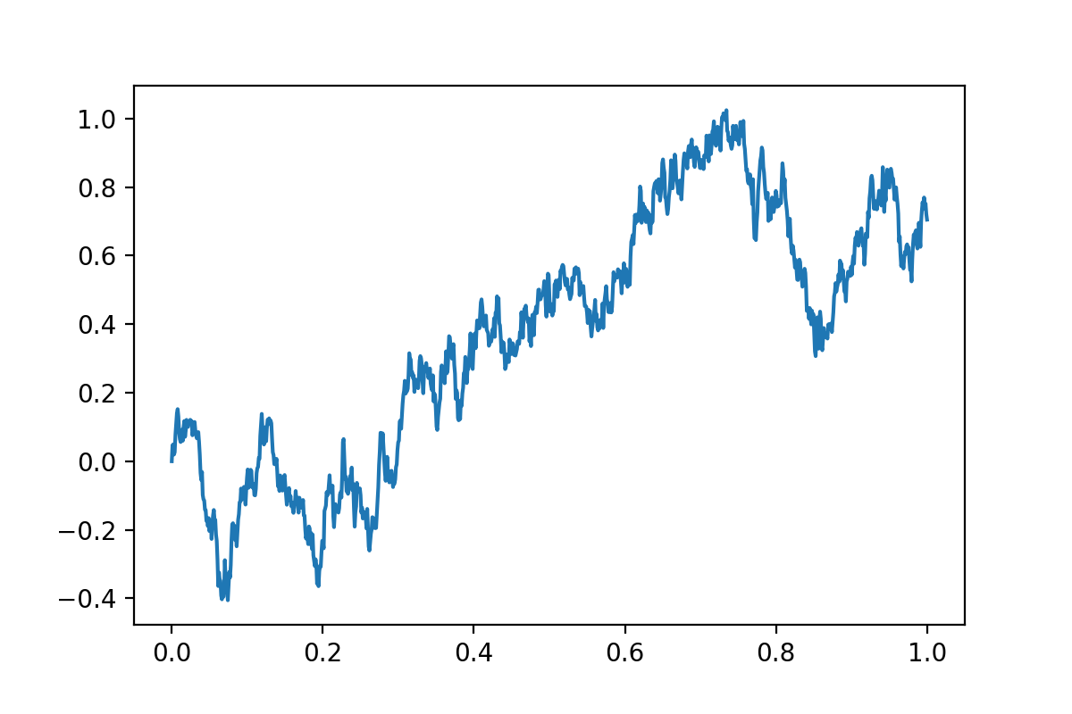 Figure 2
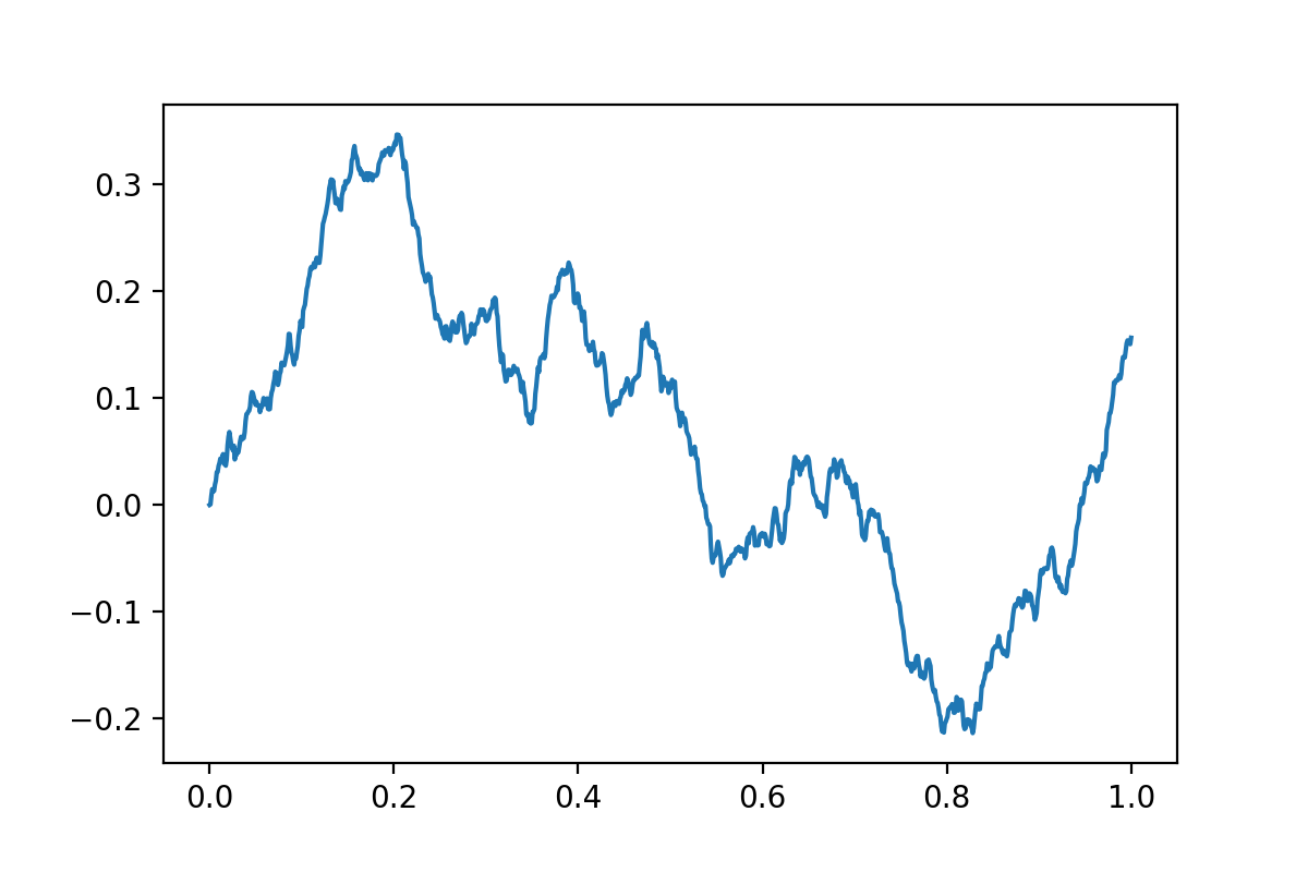 Figure 3
 Figure 4
 Figure 5
 Figure 6
 Figure 7
 Figure 8
 Figure 9
 Figure 10
 Figure 11
 Figure 12
 Figure 13
 Figure 14
 Figure 15
 Figure 16
 Figure 17
 Figure 18
Peer Reviews
No public reviews on file for this paper yet. If you reviewed it on a platform where reviews are public (OpenReview, ICLR, NeurIPS, ICML), you can paste yours below so the community can read it here.
Videos
No videos yet. Explain this paper in a talk, walkthrough, or lecture? Add one.
Sample Paths Estimates for Stochastic Fast-Slow Systems driven by Fractional Brownian Motion
Katharina Eichinger and Christian Kuehn and Alexandra Neamţu Technical University of Munich (TUM), Faculty of Mathematics, 85748 Garching bei München, GermanyTechnical University of Munich (TUM), Faculty of Mathematics, 85748 Garching bei München, GermanyTechnical University of Munich (TUM), Faculty of Mathematics, 85748 Garching bei München, Germany
Abstract
We analyze the effect of additive fractional noise with Hurst parameter on fast-slow systems. Our strategy is based on sample paths estimates, similar to the approach by Berglund and Gentz in the Brownian motion case. Yet, the setting of fractional Brownian motion does not allow us to use the martingale methods from fast-slow systems with Brownian motion. We thoroughly investigate the case where the deterministic system permits a uniformly hyperbolic stable slow manifold. In this setting, we provide a neighborhood, tailored to the fast-slow structure of the system, that contains the process with high probability. We prove this assertion by providing exponential error estimates on the probability that the system leaves this neighborhood. We also illustrate our results in an example arising in climate modeling, where time-correlated noise processes have become of greater relevance recently.
1 Introduction
Fast-slow systems naturally arise in the modeling of several phenomena in natural sciences, when processes have widely differing rates [31, 25, 23]. The standard form of a fast-slow system of ordinary differential equations (ODEs) is given by
[TABLE]
where are the fast variables, are the slow variables, is a small parameter, and are sufficiently smooth vector fields; for a more detailed technical introduction regarding the analysis of (1) we refer to Section 2.1. Here we just point out the basic aspects from the modeling perspective. First, note that if , then (1) becomes a parametrized set of ODEs, where the -variables are parameters. Taking this viewpoint, all bifurcation problems [21, 33] involving parameters naturally relate to fast-slow dynamics if the parameters vary slowly, which is often a natural assumption in applications. Second, in practice, we also want to couple many dynamical systems. The resulting large/complex system is often multiscale in time and space. For example, in the context of climate modeling [12, 26] coupled processes can evolve on temporal scales of seconds up to millennial scales. Third, fast-slow systems are the core class of dynamical problems to understand singular perturbations [51], i.e., roughly speaking singular perturbations problems with small parameters are those, which degenerate in the limit of the small parameter into a different class of equations. Combining all these observations, it is not surprising that fast-slow systems have become an important tool in more theoretical as well as application-oriented parts of nonlinear dynamics [31].
However, when dealing with real life phenomena certain random influences have to be taken into account and quantified in a suitable way [16]. The most common stochastic process used to describe uncertainty is Brownian motion . One of its key features is the memory-less or Markov property, which means that the behavior of this process after a certain time only depends on the situation at the current time . In certain applications it may be desirable to model long-range dependencies and to take into account the evolution of the process up to time . One of the most famous example is constituted by fractional Brownian motion (fBm) ; see [28] for its first use. A fBm is a centered stationary Gaussian processes parameterized by the so-called Hurst index/parameter . For one recovers classical Brownian motion. However, for and , fBm exhibits a totally different behavior compared to Brownian motion. Its increments are no longer independent, but positively correlated for and negative correlated for . The Hurst index does not only influence the structure of the covariance but also the regularity of the trajectories. Fractional Brownian motion has been used to model a wide range of phenomena such as network traffic [49], stock prices and financial markets [35, 47], activity of neurons [42, 15], dynamics of the nerve growth [39], fluid dynamics [52], as well as various phenomena in geoscience [36, 29, 41]. However, the mathematical analysis of stochastic systems involving fBm is a very challenging task. Several well-known results for classical Brownian motion are not available. For instance, the distribution of the hitting time of a level is explicitly known for a Brownian motion, whereas for fBm, one has only an asymptotic statement, according to which
[TABLE]
as goes to infinity, see [37]. Furthermore, since fBm is not a semi-martingale, Itô-calculus breaks down. Therefore, it is highly non-trivial to define an appropriate integral with respect to the fBm. This issue has been intensively investigated in the literature. There are numerous approaches that exploit the regularity of the trajectories of the fBm in order to develop a completely path-wise integration theory and to analyze differential equations. For more details, see [34, 17, 19, 20, 24] and the references specified therein. Furthermore, another ansatz employed to define stochastic integrals with respect to fBm relies on the stochastic calculus of variations (Malliavin calculus) developed in [10]. In summary, fBm is a natural candidate process to aim to improve our understanding of correlated stochastic dynamics.
Our objective here is to combine the study of fast-slow systems and fBm by starting to study stochastic differential equations of the form
[TABLE]
where we start with the case of additive noise for the fast variable(s) and assume there is a single regularly slowly-drifting variable . For , i.e., for Brownian motion, there is a very detailed theory, how to analyze stochastic fast-slow systems [31]. One particular building block - initially developed by Berglund and Gentz - uses a sample paths viewpoint [4]. This approach has recently been extended to broader classes of spatial stochastic fast-slow systems [18] and it has found many successful applications; see e.g. [3, 30, 44, 48]. Therefore, it is evident that one should also consider the case of correlated noise in the fast-slow setup [53, 22].
Our key goal is to derive sample paths estimates for fast-slow systems driven by fBm with Hurst index . We restrict ourselves to the case of additive noise and establish the theory for the normally hyperbolic stable case. Due to the technical challenges mentioned above, we need to derive sharp estimates for the exit times for processes solving certain equations driven by fBm. Exploring various properties of general Gaussian processes, we propose two variants to obtain optimal sample paths estimates.
Then we are going to apply our theory to a climate model describing the North-Atlantic thermohaline circulation forced by fractional Brownian motion. In fact, it is well-established that just using white noise modelling in climate models can be insufficient. The simple reason is that neglecting spatial and temporal correlations does not represent the statistics of large classes of underlying climate measurement data including temperature time series [27, 13], historical climate data [1, 2, 9], as well as large-scale simulation data [6]. In all these cases, an elegant way to model temporal correlations in climate science is fractional Brownian motion [9, 27, 46, 1, 54]. The reasoning to use a time correlated process can also be understood in climate dynamics in various intuitive ways. For example, in a larger-scale climate model, stochastic terms often represent unresolved degrees of freedom or small-scale fluctuations. If we consider the weather as a short-lived smaller scale effect in terms of the global long-term climate, then models for the latter must include noise with (positive) time correlations as weather patterns are positively correlated in time on short scales. Similarly, if the noise terms represent external forcing, such as input from another climate subsystem on a macro-scale, then also this input is likely to be correlated in time as there are internal correlations of the long-term behaviour of each larger-scale climate subsystem. In summary, this has motivated us to consider a model from climate dynamics as one possible key application for fast-slow dynamical systems with fractional Brownian motion. As mentioned above, in many other applications, fractional Brownian motion also naturally appears, so our modelling approach via fast-slow systems with with fBm is even more broadly applicable.
This work is structured as follows. In Section 2 we introduce basic notions from the theory of fast-slow systems and fractional Brownian motion. Furthermore, we state important estimates for the exit times of Gaussian processes which will be required later on. In Section 3, we generalize the theory of [4] by first deriving an attracting invariant manifold of the variance using the fast-slow structure of the system. Based on this manifold we define a region, where the linearization of the process is contained with high probability. In order to prove such statements, we first derive a suitable nonlocal Lyapunov-type equation for the covariance of the solution of a linear equation driven by fBm, the so-called fractional Ornstein-Uhlenbeck process. Thereafter we analyze two variants which entail sharp estimates for the exit times of this process. Furthermore, we consider more complicated dynamics and provide extensions of our results to the non-linear case, more complicated slow dynamics and finally discuss the case of fully coupled dynamics. We apply our theory to a model for the North-Atlantic thermohaline circulation and provide some simulations. Section 4 generalizes the sample paths estimates to higher dimensions in the autonomous linear case. Our strategy is based on diagonalization techniques, which allow us to go back to the one-dimensional case and apply the results developed in Section 3. For completeness, we provide an appendix which contains a detailed proof regarding the limit superior of a non-autonomous fractional Ornstein-Uhlenbeck processes. We conclude in Section 5 with an outlook of possible continuations of our results.
2 Background
2.1 Deterministic Fast-Slow Systems
In this section, we will briefly introduce the terminology of fast-slow systems. We restrict ourselves to the most important results tailored to our problem in the upcoming sections. For further details, see [31]. For the definition of the setting, all of the equations are to be understood formally. We will later add regularity assumptions sufficient to deduce important results. These also imply that the formal computation we will have performed before are valid.
Definition 2.1**.**
A fast-slow system is an (ODE) of the form
[TABLE]
where , are the unknown functions of the fast time variable , the vector fields are , and is a small parameter. The variables are called the fast variables, while variables are called the slow variables. Transforming into another time scale by defining theslow time yields the equivalent system
[TABLE]
Depending on the situation both formulations in fast and slow time may be of use. In particular, under certain assumptions, considering them for indicates a lot of information for the underlying dynamics for the case . The process for is called the singular limit. The singular limit of (3) for
[TABLE]
is called the fast subsystem. The resulting system of the slow time formulation of the fast-slow system (4) for
[TABLE]
is called the slow subsystem. The set
[TABLE]
is called the critical set. If is a manifold, it is also called the critical manifold. From now on, we assume that is a manifold given by a graph of the slow variables, i.e.,
[TABLE]
where is an open subset.
Theorem 2.2** (Fenichel–Tikhonov,[14, 50, 25, 31]).**
Let , , and their derivatives up to order be uniformly bounded. Assume that is uniformly hyperbolic. Then for an there exists a locally invariant -smooth manifold
[TABLE]
for all , where with respect to the fast variables. Furthermore, the local stability properties of are the same as the ones for .
2.2 Fractional Brownian Motion
In this section we state important properties of fBm, which will be required later on. For further details see [38, 5] and the references specified therein. We fix a complete probability space and use the abbreviation a.s. for almost surely.
Definition 2.3**.**
Let . A one-dimensional fractional Brownian motion (fBm) of Hurst index/parameter is a continuous centered Gaussian process with covariance
[TABLE]
Note that for the covariance of fBm satisfies
[TABLE]
We further observe that:
for one obtains Brownian motion; 2. 2)
for then a.s. for all . Due to this reason one always considers .
The following result regarding the structure of the covariance of fBm holds true, see [38, Section 2.3].
Proposition 2.4**.**
Let . Then, the covariance of fBm has the integral representation
[TABLE]
where the integral kernel is given by
[TABLE]
for a positive constant depending exclusively on the Hurst parameter.
We remark that for suitable square integrable kernels, one obtains different stochastic processes, for instance the multi-fractional Brownian motion or the Rosenblatt process, see [8]. We now focus on the most important properties of fBm. For the complete proofs of the following statements, see [38, Chapter 2].
Proposition 2.5** (Correlation of the increments).**
Let be a fBm of Hurst index . Then its increments are:
positively correlated for ;
- 2)
independent for ;
- 3)
negatively correlated for .
Particularly, for fBm exhibits long-range dependence, i.e.
[TABLE]
whereas for
[TABLE]
Proposition 2.6**.**
Let be a fBm of Hurst index . Then:
[Self-similarity] For
[TABLE]
i.e. fBm is self-similar with Hurst index .
- 2)
[Time inversion] \Big{(}t^{2H}W^{H}_{1/t}\Big{)}_{t>0}\overset{law}{=}(W^{H}_{t})_{t>0}.
- 3)
[Stationarity of increments] For all
[TABLE]
- 4)
[Regularity of the increments] fBm has a version which is a.s. Hölder continuous of exponent .
We conclude this section emphasizing the following result, which makes fBm very interesting from the point of view of applications, see [38, Section 2.4 and 2.5].
Proposition 2.7**.**
Let be a fractional Brownian motion with Hurst index . Then is neither a semi-martingale nor a Markov process.
2.2.1 Integration Theory for
Since fBm is not a semi-martingale, the standard Itô calculus is not applicable. Due to this reason, the construction of a stochastic integral of a random function with respect to fBm has been a challenging question, see [10, 5] and the references specified therein. However, for deterministic integrands and for the theory essentially simplifies. We deal exclusively with this case and indicate for the sake of completeness the theory of Wiener integrals of deterministic functions with respect to fBm, see [10]. Let and
[TABLE]
be the set of step functions on . For define the linear mapping
[TABLE]
Observe that defines a Gaussian random variable with
[TABLE]
where
[TABLE]
The representation of the variance can be easily verified by noting the following identity
[TABLE]
Note that is crucial here. For we can bound the -norm of as follows
[TABLE]
where we have obtained the estimate by applying Hölder’s inequality and Young’s inequality for convolutions [7, Theorem 3.9.4]. The boundedness claim now follows as for . This means that is a bounded linear operator defined on the dense subspace , so it can be uniquely extended to a bounded operator
[TABLE]
This discussion justifies the following definition:
Definition 2.8**.**
For and we set
[TABLE]
The integral process is by construction centered Gaussian. Regarding (7), its covariance can be immediately computed as follows.
Proposition 2.9** (Covariance of the integral).**
Let and for . Then
[TABLE]
2.2.2 Stochastic Differential Equations Driven by Fractional Brownian Motion
After establishing a suitable stochastic integral with respect to the fractional Brownian motion, we consider stochastic differential equations (SDEs) given by:
[TABLE]
The solution satisfies the integral formulation
[TABLE]
where the stochastic integral was constructed in Section 2.2.1. Under certain classical regularity assumptions, existence and uniqueness of solutions for (9) can be proven. For more details, see [5, Theorem D.2.4].
Theorem 2.10**.**
Let be globally Lipschitz in both variables, with and globally Lipschitz. Then for every the SDE (9) has a unique continuous solution on a.s..
In this work one case we have to consider is a time-dependent linear drift, i.e., is linear with for every and . In this case, the solution of (9) is given by the variation of constants formula/Duhamel’s formula and is called non-autonomous fractional Ornstein-Uhlenbeck process.
Theorem 2.11** (Non-autonomous Fractional Ornstein-Uhlenbeck Process).**
Let . Suppose that is globally Lipschitz and uniformly bounded, and with as well as globally Lipschitz. Then there exists an a.s. unique solution to the stochastic differential equation
[TABLE]
which satisfies the variation of constants formula
[TABLE]
Remark 2.12*.*
Note that all the results discussed in this subsection extend to higher dimensions, since all previous steps can be done component-wise. Namely, for we mention.
- (R1)
We call an -dimensional fractional Brownian motion if , where is a basis in and , , are independent one-dimensional fractional Brownian motions with the same Hurst index .
- (R2)
Naturally, existence and uniqueness of SDEs in higher dimension carry over from Theorem 2.10 under the same assumptions respectively. In particular, for coefficients with , satisfying the same assumptions as in Theorem 2.11, the solution of (10) is given by
[TABLE]
where denotes the fundamental solution of and is an -dimensional fractional Brownian motion.
2.3 Useful Estimates of Gaussian Processes
The fact that fBm is not a semi-martingale restricts the repository of known inequalities (such as Doob or Burkholder-Davies-Gundy) to establish sample paths estimates. A crucial property of fBm we shall exploit is its Gaussianity. In this section we will describe some useful estimates for exit times of certain Gaussian processes, which will be helpful for our analysis in the upcoming sections.
We first state the next auxiliary result regarding the Laplace transform of a Gaussian process. This was established in [11] by means of Malliavin calculus.
Lemma 2.13**.**
(Proposition 3.5 [11])* Let be a centered Gaussian process with and covariance function satisfying the following conditions:*
- i)
* exists and is continuous as a function on ,* 2. ii)
* for all ,* 3. iii)
* for all ,* 4. iv)
* a.s.*
Then for any :
[TABLE]
where and .
In addition, we require the following form of Chebychev’s inequality.
Lemma 2.14**.**
Let be measurable, a random variable and . Then
[TABLE]
Proof.
Under these assumptions we have
[TABLE]
Taking expectation in the above inequality yields the result. ∎
Lemma 2.15**.**
Let and be a centered Gaussian process with satisfying the assumptions i)-iv) of Lemma 2.13. Then, for its exit time , the following estimate holds:
[TABLE]
Proof.
Applying Lemma 2.14 for , and we can bound the probability together with (11) as follows:
[TABLE]
for all . Optimizing over and noticing that proves the statement. ∎
The previous lemma established a Bernstein-type inequality solely relying on certain properties of the covariance function of Gaussian processes. Another useful estimate is given by [40, Theorem D.4], which is based on Slepian’s Lemma [45].
Theorem 2.16**.**
Let and be a centered Gaussian process with a.s. continuous trajectories. Assume that is a.s. mean-square Hölder continuous, i.e. there are constants and such that
[TABLE]
Then there exists a constant such that for and
[TABLE]
where .
This estimate can be sharpened if we restrict ourselves to the interval of interest.
Corollary 2.17**.**
Let and be a centered Gaussian process with a.s. continuous trajectories. Assume that is a.s. mean-square Hölder continuous, i.e. there are constants and , such that
[TABLE]
Then there exists a constant such that for and
[TABLE]
where .
Proof.
with satisfies the assumptions of Theorem 2.16 on . ∎
3 The One-Dimensional Case
In this section, we investigate the dynamics of a planar stochastic fast-slow system driven by fractional Brownian motion with Hurst parameter :
[TABLE]
Its equivalent formulation in slow time, i.e. for is
[TABLE]
using the self-similarity of fBm (6). We are interested in the normally hyperbolic stable case and therefore make the following assumptions.
Assumption 3.1**.**
Stable Case
Regularity:* The functions and , as well as all their existing derivatives up to order two are uniformly bounded on an interval or , , by a constant .* 2. 2)
Critical manifold:* There is an such that*
[TABLE]
for all . 3. 3)
Stability:* For there is such that*
[TABLE]
for all .
Under these assumptions, (12) has a unique global solution according to Theorem 2.10. Furthermore, the deterministic system, i.e., for , given by
[TABLE]
has an asymptotically slow manifold for small enough due to Fenichel-Tikhonov (Theorem 2.2). We expect that, given small noise , the trajectories of (12) starting sufficiently close to remain in a properly chosen neighborhood of for a long time with high probability. Our goal will be to make this idea rigorous by pursuing the following steps. We first linearize the system around the slow manifold to get an SDE describing the deviations induced by the noise. This helps us obtain a simple description of a suitable neighborhood by using the fast-slow structure inherited by the variance of the system. Then, using this neighborhood, we deduce sample paths estimates for the linear case starting on the slow manifold. To complete the discussion we generalize the result to the non-linear case starting sufficiently close to the slow manifold, that is, such that in the deterministic case solutions are still attracted by the slow manifold. This general strategy inspired by [4], where a similar system driven by Brownian motion (Hurst parameter ) is analyzed. Yet, the several techniques used in [4] do not generalize to fBm.
3.1 The Linearized System
The deterministic system
[TABLE]
has an asymptotically stable slow manifold due to Fenichel-Tikhonov (Theorem 2.2). As already outlined, our first step is to examine the behavior of the linearized system around . For a solution of we set . Then satisfies the equation
[TABLE]
where
[TABLE]
by Taylor’s remainder theorem. Due to the uniform boundedness of the derivatives of one can show that the -term is negligible on finite time scales as Therefore, we restrict ourselves without loss of generality to the analysis of the linearization
[TABLE]
Examining the process starting on the slow manifold now corresponds to investigating the unique explicit solution of (14) for initial value , which is given by the fractional Ornstein-Uhlenbeck process (recall Theorem 2.11)
[TABLE]
where . In order to define a proper neighborhood, where the fractional Ornstein-Uhlenbeck process is going to stay with high probability, we use the variance as an indicator for the deviations at time . According to Proposition 2.9, the variance is given by
[TABLE]
As we would like to see dynamics of , we rescale it by to get rid of the small parameter , which only changes the order of magnitude of the system. It turns out that inherits the fast-slow structure from the SDE, which yields a particularly simple approximation of the variance.
Proposition 3.2**.**
The so-called renormalized variance satisfies the fast-slow ODE
[TABLE]
In particular, there is a (globally) asymptotically stable slow manifold of the system of the form
[TABLE]
Proof.
Differentiating yields
[TABLE]
In order to be able to take the singular limit and apply Fenichel-Tikhonov (Theorem 2.2) we need to prove sufficient regularity in ; continuous differentiability will be enough for the approximation of the slow manifold with the critical manifold up to order . To do this, rewrite the integral by substituting
[TABLE]
To see that the right hand side of (15) is continuously differentiable in it is sufficient to check it for the integral term
[TABLE]
which has an existing limit for because the exponential term goes to [math] faster than the polynomial term diverges. Now taking the singular limit gives the slow subsystem
[TABLE]
The critical manifold is hence given by
[TABLE]
Using integration by parts we can rewrite , so that the critical manifold can also be written as
[TABLE]
By Theorem 2.2, the ODE (15) has a solution of the form
[TABLE]
which is asymptotically stable due to Assumption 3.1 3. This stability property is even global in this case because the ODE (15) is linear. ∎
As expected, the critical manifold depends on the Hurst parameter . For we have . This means that the only possible structural change of the critical manifold under variation of is induced by the factor . Furthermore, as for , the slow subsystem for reads
[TABLE]
which coincides with the slow subsystem we would obtain in the case of Brownian motion noise, which exactly corresponds to .
Remark 3.3*.*
The proof of Proposition 3.2 only shows that is in and in the time . Depending on the properties of we expect to even have higher regularity. However, this fact is not required in the following considerations.
Proposition 3.2 already states that the slow manifold is a good indicator for the size of the set we are looking for as (as a solution of (15) with initial datum ) is attracted by the slow manifold. In this particular case we can explicitly state the exponentially fast approach due to the structure of the linear equation
[TABLE]
where . Even more is known about the properties of . Due to the uniform boundedness assumption on and we get that the difference between and is actually in uniform This implies that for small enough there are and such that
[TABLE]
The goal is now to prove that the stochastic process is concentrated in sets of the form
[TABLE]
To get a better understanding of what to expect, note that the probability that leaves at time can be bounded by using the inequality , which holds for any centered Gaussian random variable . This further leads to
[TABLE]
Of course, the probability that has exited in the interval at least once
[TABLE]
is larger, where is the first time has exited . We will present a few approaches to estimate this probability in the following, using the inequalities we have established in Section 2.3. The increase of probability compared to (18) is simply indicated by the prefactor of .
Remark 3.4*.*
It could also have been possible to define the neighborhood by considering the critical manifold , i.e. to define
[TABLE]
This will yield the same bounds on the exit times, which we will establish in the following because the difference between and is only in which is of the same order as the order we obtain by approximating with the slow manifold anyways.
3.1.1 Variant 1
The first approach is based on the result on exit times of Gaussian processes with sufficiently regular and increasing covariance function, as stated in Lemma 2.15.
Theorem 3.5**.**
Let Then under Assumption 3.1 for any the following estimate holds true for sufficiently small
[TABLE]
Proof.
In order to apply the estimate given in Lemma 2.15 to our problem observe that may not satisfy all the assumptions. First of all we need well-definedness of the Ornstein-Uhlenbeck process over the whole non-negative real line ; this is guaranteed by Assumption 3.1. In addition, we consider the process given by . Note that the event that exceeds a certain level corresponds exactly to the event of exceeding , that is . Unfortunately this observation does not carry over to and . In fact, a priori we only have the relation , which yields a too strong estimate in the end as we are increasing the variance by an exponentially increasing factor, while maintaining the same exit level! A way to overcome this is to partition the interval to suitable subintervals to obtain the relation . This partition will also turn out to be useful to control the variance with the slow manifold in the exponential of the estimate. The covariance of is given by
[TABLE]
By the theorem for differentiation of parameter dependent integrals we deduce that exists and is continuous in . Furthermore, for all is an immediate consequence of the fundamental theorem of calculus as the integrand is always greater equal than [math]. This already implies assumption (i) und (ii) of Lemma 2.15. For assumption (iii) it suffices to observe that
[TABLE]
is a Gaussian process with nonzero variance. Assumption (iv) follows by Corollary A.2. This implies that satisfies a Bernstein-type inequality due to Lemma 2.15
[TABLE]
After having established this result, we can proceed as in the proof of Proposition 3.1.5 [4]. For let be a partition containing the interval such that
[TABLE]
(Note that is possible. But this only increases the estimate on the probability slightly. As we would like to optimize over in the end, it does not make sense to fix it to obtain .) For each we have
[TABLE]
where the last inequality follows by , which is proven in Lemma 3.6. Now by subadditivity of the probability measure
[TABLE]
where the last inequality is due to . Due to monotonicity of , it suffices to minimize
[TABLE]
in order to find the minimal value of this estimate. Optimizing over hence yields
[TABLE]
which finishes the proof. ∎
Lemma 3.6**.**
The slow manifold satisfies .
Proof.
Note that
[TABLE]
satisfies the corresponding invariance equation for the fast-slow ODE (15) up to error This implies that . Plugging this representation of into the ODE (15) yields directly . ∎
3.1.2 Variant 2
The second approach uses the fact that is mean-square Hölder continuous. This is also going to enable to control the deviations based upon Theorem 2.16.
Theorem 3.7**.**
Let Then under Assumption 3.1 there is a constant , such that for any the following estimate holds true for sufficiently small
[TABLE]
where
Proof.
Let . In order to apply Theorem 2.16 we have to prove mean-square Hölder continuity of . For
[TABLE]
Lipschitz continuity of for arbitrary (with Lipschitz constant , where ) yields for (20)
[TABLE]
Similarly we can show for (21)
[TABLE]
Last but not least (22) can be estimated as follows
[TABLE]
By combining the three estimates we obtain that, for a constant , it holds
[TABLE]
Let be a partition of the interval such that
[TABLE]
For each we have by Corollary 2.17 for
[TABLE]
where the last inequality follows by , see Lemma 3.6. This yields by the subadditivity of the probability measure
[TABLE]
Therefore, the proof is finished. ∎
3.2 Comparison of the two Variants
In this section, we will compare the two variants in view of varying the noise intensity given by and the time scale parameter . In order to better understand what to expect under these variations we first heuristically describe their effect on the underlying SDE
[TABLE]
We can directly see that a smaller reduces the intensity of the fraction Brownian motion noise. In particular, as is decreasing, the probability that exits on some interval should become smaller. For a smaller the attraction towards the slow manifold becomes stronger, however also the noise intensity increases. We expect small deviations if is sufficiently small.
Suppose we are in the situation of Theorem 3.5 and Theorem 3.7. To simplify the comparison the results of both variant 1
[TABLE]
where , are displayed here. Unfortunately, we do not know the dependence of on the other parameters, so we can only do a qualitative comparison up to some extent. By looking at the proof of Theorem 3.7 we guess that is increasing in , so that we assume for the forthcoming analysis that is increasing in , decreasing in and increasing in . In variant 1, we see the same interplay of and as already observed in the analysis of because the exponential dominates the linear term in the prefactor, and the same holds true for variant 2 as long as (for to remain relatively small), which is true in many applications. For the estimate in variant 1 becomes larger, whereas in variant 2 it does not seem to have a huge effect on the bound. However, the increase might be hidden in . As the time increases, it obviously becomes more likely that has already exited at least once. In variant 1 this increase is displayed linearly in as is uniformly bounded and thus . Variant 2 shows an increase which is at least linear in because might be increasing in as well. This means that in variant 1 we have to pick large enough such that is significantly larger than . For variant 2 we have to choose in a suitable way that is larger than . Although we cannot prove it, it seems that variant 1 yields a sharper bound. Last but not least, note that the estimate in variant 1 coincides with the estimate derived for the Brownian motion case, see [4, Proposition 3.1.5]. The dependence of the Hurst parameter is completely hidden in the structure of the neighborhood , which depends on the slow manifold. This also intuitively makes sense because we are “almost” dividing by the variance. Furthermore, in the Brownian motion case this estimate is quite close to the actual distribution of the exit time , see [4, Theorem 3.1.6] and the comments below.
3.3 Back to the Original System
Now that we have convinced ourselves that the most promising estimate is given in Theorem 3.5 it remains to generalize the result to different scenarios which may be of interest.
3.3.1 The Nonlinear Case
Recall that we have rewritten the SDE (13) satisfied by the deviations around the slow manifold
[TABLE]
with being the linear drift term and containing the (possible) nonlinearities of the equation satisfying . As we expect that the nonlinear term does not influence the deviations too strongly near the critical manifold, we use the same neighborhood . This in particular implies that we keep the same simple description of it, which we have derived in Proposition 3.2. The bound on will help us to control it inside of . For the case that is starting on the slow manifold, i.e. we obtain:
Theorem 3.8**.**
Let . For sufficiently small it holds
[TABLE]
where .
Proof.
As previously motivated before we treat the nonlinear drift term as perturbation of the linear system, i.e. split the solution of (13)
[TABLE]
where is a solution to the linear system, which we have already studied in detail, and
[TABLE]
Then for , we consider
[TABLE]
It remains to prove that is small. Observe that due to continuity of we have for
[TABLE]
This enables us to control inside of thanks to the bound on the Taylor remainder term
[TABLE]
Hence, choosing results in . Note that this is choice is possible as long as , which is in , so requiring is possible. Indeed, the choice of is usually even “smaller” than , so that . Applying Theorem 3.5 to now yields the claim. ∎
Remark 3.9*.*
With this approach we lose some accuracy ( instead of ) in the exponential. This has more effect on the increase of probability than in the prefactor. To overcome this difficulty it might be better to adapt the neighborhood depending on the nonlinearities.
3.3.2 Behavior Close to the Slow Manifold
For the deterministic system we get in the case of a uniformly asymptotically stable slow manifold that solutions starting close to it are attracted exponentially fast. Given low enough noise intensity a similar behavior can be observed in the noisy system, i.e., solutions have small deviations around the deterministic solution and after some (small) time we can again observe small deviations around the slow manifold.
Theorem 3.10**.**
Let , . There is and some time such that the solutions of (12) with initial condition satisfying
[TABLE]
are attracted by the slow manifold. That is, up to time the solution is close to the deterministic solution
[TABLE]
where the denotes the different values due to linearization around instead of the slow manifold . After we obtain almost the same behavior as in the case where , i.e. for
[TABLE]
Proof.
Exponentially fast attraction means that there are constants such that for with it holds
[TABLE]
Consider an initial value with and denote by the solution to the deterministic system () in (12). Instead of linearizing around , like we did in (13), we linearize it around This procedure yields qualitatively the same linearization, with instead of or respectively , see discussion before, and adapted accordingly. In particular, even for the nonlinear case we obtain by Theorem 3.8
[TABLE]
where and Choose such that for distance
[TABLE]
that is . Furthermore, we have by the mean value theorem
[TABLE]
for some So that for
[TABLE]
We want this distance to be of order at most , so that in total Then, up to time , we can use the estimate above for close to its deterministic solution. And after the process is already close to the slow manifold and its dynamics, so it makes sense to look at the deviations around . Splitting again
[TABLE]
Choosing we obtain Furthermore, since , we have
[TABLE]
which finishes the proof. ∎
3.3.3 More Complicated Slow Dynamics
So far, we have considered the case where the slow dynamics is completely uniform and regular, i.e.,
[TABLE]
However, in applications many interesting systems contain more complicated slow variables. In fact, this is particularly relevant if one wants to reduce the dynamics to the slow manifold. The reduced equation usually qualitatively describes the dynamics of the slow variables around the slow manifold quite well. This section will clarify that the theory developed so far can be extended to more complicated slow dynamics in two steps. We first generalize our result to deterministic slow dynamics, which may also influence the diffusion term and then consider a fully coupled system.
Deterministic Slow Dynamics
Hence, we consider systems of the form
[TABLE]
We have to adapt the assumptions a bit.
Assumption 3.11**.**
Stable Case, Non-trivial Slow Dynamics
Regularity:* The functions , and , as well as their derivatives up to order are uniformly bounded on an open subset by a constant . Here is the projection onto the second coordinate.* 2. 2.
Critical manifold:* There is an for open such that*
[TABLE]
is a critical manifold of the system (23). 3. 3.
Stability:* For there is such that*
[TABLE]
for all . 4. 4.
Global existence:* The solutions of (23) are defined for all .*
Under these assumptions the system (23) has an attracting slow manifold
[TABLE]
where due to Theorem 2.2 (Fenichel-Tikhonov). (Again, this is uniform in .) We linearize the fast variable around . For a solution of set , then satisfies the equation
[TABLE]
where due to Taylor’s remainder theorem
[TABLE]
Now we can proceed as in the case for trivial slow dynamics by first considering solutions starting on the slow manifold, i.e. , and using the terms
[TABLE]
This way we obtain the same qualitative bound (also for the nonlinear case) as before, which also coincides with intuition, as more involved dynamics on the slow manifold should not influence the attracting behavior of it.
Fully Coupled Dynamics
Now that we have seen the idea how to generalize to more complicated dynamics we give an exposition of the more general case, where the slow variables may even be random, particularly be perturbed by fBms with different Hurst parameters . We consider the following system
[TABLE]
which will turn out to be interesting in applications, see Section 3.4. The following assumptions will suffice to obtain a qualitatively similar result to the one-dimensional case, analyzed in Section 3.
Assumption 3.12**.**
Stable Case, fully Coupled System
Regularity:* The functions and as well as their derivatives up to order are uniformly bounded on an open subset .* 2. 2.
Critical manifold:* There is an for open such that*
[TABLE]
is a critical manifold of the system (25). Here is the projection onto the second coordinate. 3. 3.
Stability:* For there is such that*
[TABLE]
for all . 4. 4.
Global existence:* The solutions of (25) are defined for all .*
Remark 3.13*.*
Note that the theory discussed in Section 2.2.1 does not provide the technical details regarding the existence and uniqueness of solutions for coupled systems driven by fractional Brownian motion. However, this can be extended to systems of the form (25). We refer to [38, Theorem 3.3] for further details.
Similarly as before the system (25) has an attracting slow manifold given by
[TABLE]
where due to Theorem 2.2, where again the -term is uniform in . The strategy to establish sample paths estimates for (25) is to successively linearize both fast and slow variables around their deterministic counterpart (i.e. the solution for ) denoted by , . The deviations are then described by
[TABLE]
They satisfy the following SDE, whose form is obtained by successively applying Taylor’s theorem ( always stands for the appropriate intermediate value)
[TABLE]
where
[TABLE]
so that where is uniform in the variables due to the uniform boundedness assumption.
[TABLE]
where
[TABLE]
In particular the nonlinearity term satisfies for some (again uniform in the variables)
[TABLE]
In order to prove that is concentrated in the neighborhood around the slow manifold with high probability define the exit times
[TABLE]
Then we partition the event of in the following way
[TABLE]
Note that the first probability is of the form
[TABLE]
By the same technique used to prove Theorem 3.8 we get
[TABLE]
which is valid as long as It remains to estimate . This issue is however tightly linked to investigating the behavior of non-stable or even non-hyperbolic dynamics under fractional noise because we have no additional assumptions on the slow dynamics. In the event we conjecture that a reduction to the slow variables should be possible. The reduced equation is then given by
[TABLE]
which will be illustrated by the simulations presented at the end of Section 3.4.
3.4 Example
We consider the climate model analyzed in [4, Section 6.2.1]. It is a simple model describing the difference of temperature and salinity between low latitude ( ) and high latitude ( ) by a system of coupled differential equations
[TABLE]
Here stands for the relaxation time of to its reference value , is the freshwater flux, the depth of the ocean, a reference salinity. Furthermore, is the diffusion timescale, the Poiseuille transport coefficient and the volume of the box the system is contained in. The influence of external sources, internal fluctuations, and/or microscopic effects can be incorporated into the model via noise terms. For example, daily weather variations certainly influence the temperature and salinity . Yet, a precise/detailed modelling of these terms would be far too expensive computationally and would make the model intractable analytically. We know, as discussed in the introduction to this work, that using white noise generally does not represent temperature fluctuations correctly but these are usually positively correlated. Since we have no further basic knowledge of the stochastic process it is quite natural to start by considering fBm with Hurst index . This allows us to model Gaussianity and positive correlations in time. After transforming our model into dimensionless variables , , rescaling time by and taking into consideration fractional noise with Hurst parameter , this yields the system
[TABLE]
where , , and . Note that the previous system is of the form (25). We consider the solution on a bounded time interval , to ensure the uniform boundedness of the corresponding functions, as imposed in Assumption 3.12.
The slow subsystem of the deterministic system is given by
[TABLE]
In particular, it has a normally hyperbolic critical manifold, namely
[TABLE]
which is even stable, as By Theorem 2.2 there exists an invariant manifold
[TABLE]
In order to apply the estimate from Theorem 3.5 note that , so that
[TABLE]
Hence we have
[TABLE]
By Proposition 3.2 there is an attracting slow manifold for the variance of the form
[TABLE]
We conclude that, in the case that is deterministic, sample paths starting on the slow manifold are concentrated in the set
[TABLE]
or, more precisely, for and initial data
[TABLE]
Figure 1 indicates that for small enough noise the dynamics around the slow manifold should be governed by the equation
[TABLE]
In (28) is a fixed parameter, while is proportional to the freshwater flux. It can be hence treated as a slowly varying parameter compared to the rescaled salinity. By setting and we obtain another fast slow system subject to some noise
[TABLE]
where In particular, we can apply our theory again on the two stable branches of the new slow manifold. We simulate now the reduced equation, similarly to [30, Section 7.1], where the same system was considered with respect to the Brownian motion. The results for two different Hurst parameters (i.e. and ) are illustrated in Figure 2 and 3.
4 The Multi-Dimensional Case
In this section, we make the first steps towards extending our theory to the multi-dimensional case. Note that we keep the same notation as for the one-dimensional objects. We start again with uniform slow dynamics and consider the fast-slow system system in slow time
[TABLE]
under the following assumptions. Let .
Assumption 4.1**.**
Stable Autonomous Multi-Dimensional Case
Regularity:* The function , as well as its derivatives up to order are uniformly bounded by a constant on an interval or , .* 2. 2.
Critical manifold:* There is an such that*
[TABLE]
for all . 3. 3.
Stability:* The critical manifold is asymptotically stable, i.e. the Jacobian matrix*
[TABLE]
only contains eigenvalues with negative real part. In addition, its linearization is independent of time, i.e. 4. 4.
Noise:* is an -dimensional fractional Brownian motion.*
These assumptions guarantee the existence and uniqueness of (30) due to Remark (R2)(R2). Furthermore, recall that under these assumptions there is a slow manifold
[TABLE]
due to Fenichel-Tikhonov (Theorem 2.2). We start again by examining the behavior of the linearized system around . For a solution of set , then satisfies the equation
[TABLE]
where
[TABLE]
with being the operator norm with respect to the Euclidean norm. For simplicity, we analyze the linearization with being the drift term instead of , i.e. we consider
[TABLE]
The solution for ( starting on the slow manifold ) is given by
[TABLE]
Its covariance (matrix) can be computed as
[TABLE]
In the same way as in the one-dimensional case the rescaled covariance inherits the fast-slow structure.
Proposition 4.2**.**
The so-called renormalized covariance satisfies the fast-slow ODE
[TABLE]
where
[TABLE]
In particular, there is an (even globally) asymptotically stable slow manifold of the system of the form
[TABLE]
where
[TABLE]
Proof.
We again differentiate to obtain the ODE
[TABLE]
where
[TABLE]
In order to be able to take the singular limit and apply Fenichel-Tikhonov (Theorem 2.2) we need to prove at least one times continuous differentiability in . To do this, rewrite by substituting
[TABLE]
This implies continuity in To see that the right hand side of (34) is continuously differentiable in it is sufficient to check it for the integral
[TABLE]
where the limit for exists because the exponential term dominates the polynomial term in The slow subsystem hence reads
[TABLE]
where
[TABLE]
This is a Lyapunov equation, and according to Lemma 4.4 it has the unique solution
[TABLE]
By Fenichel-Tikhonov (Theorem 2.2) we conclude that there is an asymptotically stable manifold of the form
[TABLE]
Note again that the stability property, which carries over from the critical manifold, is even global due to linearity of the ODE (34). ∎
Remark 4.3*.*
We need that the linearization (32) is autonomous in this section for taking the singular limit in (36). In the non-autonomous case we need to compute the limit of for We suspect that
In order to investigate a multi-dimensional Lyapunov-Equation, we rely on the following result, see [4, Lemma 5.1.2].
Lemma 4.4** (Lyapunov Equation).**
Let and with eigenvalues and Then the operator defined by
[TABLE]
has eigenvalues of the form In particular, L is invertible if and only if and don’t have any common eigenvalue. Moreover, if all eigenvalues of and have negative real part, then for any the unique solution of the so-called Lyapunov equation is of the form
[TABLE]
Note again that due to the linearity of the operator the rescaled covariance as solution of (34) with starting value satisfies the following equation
[TABLE]
which explicitly depicts the exponentially fast approach of the covariance towards the slow manifold, as it could have been already concluded by Fenichel-Tikhonov (Theorem 2.2). This justifies the choice of our neighborhood this time, depending on the critical manifold
[TABLE]
As already previously mentioned in Remark 3.4 choosing the neighborhood depending on the critical manifold instead of the slow manifold does not worsen our estimates. So we expect the same to be true in the higher dimensional case. Therefore, we have used the critical manifold (which is time-independent in our case) this time because our strategy depends on diagonalizing, and we do not spell out the additional technical details regarding the -term.
4.1 Estimates on the Deviations
4.1.1 No Restrictions on the Linearization
The proof of Theorem 3.7 can be immediately extended the multi-dimensional case by proving the mean-square Hölder continuity in each component of the covariance.
Lemma 4.5**.**
Let , then there is a constant such that
[TABLE]
Proof.
Let , then
[TABLE]
Since only has eigenvalues with negative real part we have for
[TABLE]
and for ,
[TABLE]
where This enables us to prove the result similarly as in the one-dimensional case, i.e. a straightforward calculation using the last result now shows the required Hölder bounds by estimating (38)-(41). ∎
The mean-square Hölder continuity of implies the same for each component. Hence, we can establish the following qualitative result.
Theorem 4.6**.**
Let Then under Assumption 4.1 there is a constant such that for the following estimate holds true for small enough
[TABLE]
where with and denote the (time-independent) eigenvalues of
Proof.
Note that the critical manifold is symmetric and in the autonomous case it is time independent in addition. This implies that it is diagonalizable with respect to an orthogonal matrix (independent of time). Let , where denotes the -th row of and be the corresponding eigenvalues. This enables us to reduce the problem to the estimate of the one-dimensional problem, using the notation
[TABLE]
We have already proven that is mean-square Hölder continuous in Lemma 4.5, which directly implies the same property for the components in the -coordinate system. This means that we can apply Theorem 2.16 for . This leads to
[TABLE]
Now note that (37) written in the -th component in the -coordinate system reads as
[TABLE]
This further implies
[TABLE]
Summing over the dimensions yields
[TABLE]
and this finishes the proof. ∎
In the case when is normal we get a nice description of the . The corresponding -th component of the diagonalized critical manifold results in
[TABLE]
4.1.2 Symmetric Linearization
From now on, we consider the case when is a symmetric matrix (i.e. ). The reason for this restriction is that in the following the proves to bound the probability of exiting the neighborhood up to time
[TABLE]
is based on linearizing the underlying system and understanding the structure of the eigenvalues of the covariance. We actually require normality of for this strategy to work as it is sufficient to use the functional equality of the matrix exponential. Furthermore, inherits the normality structure, which is a necessary and sufficient criterion to characterize the eigenvalues of . To be able to generalize the result of variant 1 it is crucial that the eigenvalues of are all real. These two criteria already imply that is symmetric. In particular, we see that the critical manifold is of the form
[TABLE]
Thanks to the discussion above the we can consider the diagonalization . Its -th () diagonal component is given by
[TABLE]
Similarly we can rewrite the covariance
[TABLE]
and diagonalize it with respect to the same and consider its -th () component
[TABLE]
We obtain the following result
Theorem 4.7**.**
Let Then under Assumption 4.1 and if is in addition symmetric with real eigenvalues there is a constant such that for the following estimate holds for small enough
[TABLE]
where
Proof.
Let , where denotes the -th row of Now
[TABLE]
Due to the normality of (inherited by ) the Gaussian process has variance
[TABLE]
In particular, we can show that the process satisfies the assumptions of Lemma 2.15, so that we can apply the Bernstein-type inequality. (The proof is completely analogous as in the one-dimensional case, see proof of Theorem 3.5.) To get a relation between the -th value of the diagonalized covariance and the corresponding component of the critical manifold consider (37) in the -coordinate system
[TABLE]
as is actually independent of time in our case. Now, we can use the same strategy as variant 1 in the one dimensional case for each For let be a partition containing the interval such that
[TABLE]
We start by estimating the probability of the exit time on for
[TABLE]
Taking the union of the events that has exited in and using the subadditivity of the probability measure, yields
[TABLE]
Finding the minimal bound with respect to now corresponds to optimizing
[TABLE]
due to the monotonicity of . The optimal value is achieved for
[TABLE]
Plugging this in the estimate gives the bound for the -th component
[TABLE]
Summing over the dimensions
[TABLE]
where The optimal value is now attained by choosing This yields
[TABLE]
The proof is complete. ∎
Due to the symmetry of we could have diagonalized the SDE in the beginning (i.e. look at it in the -coordinate system) and done the whole theory established in Chapter 2 to get the existence of a slow manifold for , which is of the form
[TABLE]
However, we decided to use the results on the higher dimensional systems as much as possible to clearly indicate which steps of the proof can be generalized to more general classes of matrices beyond symmetric ones.
5 Outlook
This work provides a first step towards the investigation of fast-slow systems driven by fBm using sample paths estimates. So far we have examined the behavior close to a normally hyperbolic attracting invariant manifold in finite dimensions. Numerous extensions could be considered as next steps.
Having covered the uniformly attracting case, it is then natural to conjecture that there are scaling laws for the fluctuations as fast subsystem bifurcation points are approached, i.e., when hyperbolicity is lost. These results are available in the fast-slow Brownian motion case [30]. However, even when the fast dynamics is dominated by nonlinear terms [43] or one considers fast-slow maps with bounded noise [32] using modified proofs and additional technical tools it is possible to save many results. This robustness of the scaling laws near the loss of normal hyperbolicity leads one to conjecture that it will still be possible to prove such results for the fast-slow fBm case when .
However, the analysis of fast-slow systems for is expected to be more complicated due to several reasons. First of all, a different integration theory has to be considered, see for instance [10, 5]. Furthermore, the kernel (8) we have used to develop an approximation of the variance by means of the slow manifold has a non-integrable singularity for . Last but not least, Bernstein-type inequalities as established in Lemma 2.15 do not hold true anymore, since the covariance function of the fractional Brownian motion is negative. Consequently, one has to develop completely different techniques in this case. Another related extension would be to analyze the dynamics of fast-slow systems driven by multiplicative noise. This issue, however, requires a more general theory than Itô-calculus because the fractional Brownian motion is not a semi-martingale.
Furthermore, one could consider other stochastic processes with memory. More precisely, one could think of other stochastic processes whose covariance functions are represented by
[TABLE]
for suitable square integrable kernels , recall (5). Beyond fBm, further examples in this sense are the multi-fractional Brownian motion or the Rosenblatt process [8]. However, the analysis of fast-slow systems in this case is a challenging question, since these processes do not have in general stationary increments and are no longer Gaussian (as e.g. Rosenblatt processes).
Finally, one can also broaden the scope of the applications. Although climate dynamics is certainly a very important topic, where time-correlated noise is well-motivated by data such as temperature measurements, it is not the only possible application. Other areas, where fast-slow systems with fBm could be considered are financial markets. For example, assets could be modelled as fast variables influenced by fBm stochastic forcing, while the slow variables are political/social factors influencing the market, which change on a much slower time scale in many cases. Similar remarks and examples of concrete applications are likely also exist in many contexts in neuroscience, ecology and epidemiology, where stochastic fast-slow systems with Brownian motion are already used frequently.
Acknowledgments: CK & AN would like to thank the German Science Foundation (DFG) for support via grants (KU 3333/2-1) and (GN 109/1-1). CK would like to thank the VolkswagenStiftung for support via a Lichtenberg Professorship. The authors are extremely grateful to Professor Andrey Dorogovtsev for valuable suggestions and for pointing out Theorem A.1. CK also acknowledges partial support of the EU within the TiPES project funded the European Unions Horizon 2020 research and innovation programme under grant agreement No. 820970. The authors thank the referees for the valuable suggestions.
Appendix A On the Limit Superior of Gaussian Processes
The following proof has been developed in personal communication with Professor Andrey Dorogovtsev.
Theorem A.1**.**
Let be a centered Gaussian process with covariance function satisfying
* for * 2. 2.
* for all *
Then
[TABLE]
Proof.
We aim to construct a sequence of independent random variables inductively to apply the Borel-Cantelli lemma. The strategy is highly based on the fact that for Gaussian random variables independence is equivalent to zero covariance. Let Given we apply Gram-Schmidt orthogonalization to the variables in to obtain uncorrelated and normalized random variables satisfying for each
[TABLE]
where the coefficients and only depend on the on the values for by construction. Now for any we can project on the space
[TABLE]
Observe that by construction is uncorrelated, and hence independent, of the the variables This holds in particular if we choose with
[TABLE]
where the latter is possible because for Inductively we get for each
[TABLE]
For the sequence of independent random variables
[TABLE]
because by assumption. By the Borel-Cantelli lemma we obtain
[TABLE]
Now note that as as for any
[TABLE]
This implies that
[TABLE]
as required. ∎
Now we can apply this result to our setting.
Corollary A.2**.**
Under the Assumptions of Theorem 3.5 we have
[TABLE]
Proof.
Define Then by construction. To prove the second assumption of Theorem A.1, observe that
[TABLE]
Now note that is bounded for This means it suffices to prove for every
[TABLE]
The correlation function is given by
[TABLE]
where Let Then there is such that for
[TABLE]
Now choose such that for all
[TABLE]
where we have used the semi-group property of Putting this together we get for all
[TABLE]
Now, Theorem A.1 proves the claim. ∎
Remark A.3*.*
Note that one cannot directly apply classical probabilistic results such as the Borel-Cantelli Lemma, law of iterated logarithm or ergodic theorems to prove Corollary A.2, since the process has neither stationary nor independent increments.
The reference list from the paper itself. Each links out to its DOI / PubMed record.
- 1[1] Y. Ashkenazy and D.R. Baker and H. Gildor and S. Havlin. Nonlinearity and multifractality of climate change in the past 420,000 years. Geophysical research letters , 30(22), 2003.
- 2[2] L. Barboza and B. Li and M.P. Tingley and F.G. Viens. Reconstructing past temperatures from natural proxies and estimated climate forcings using short-and long-memory models. The Annals of Applied Statistics , 8(4):1966–2001, 2014.
- 3[3] N. Berglund and B. Gentz. The effect of additive noise on dynamical hysteresis. Nonlinearity , 15(3):605–632, 2002.
- 4[4] N. Berglund and B. Gentz. Noise-Induced Phenomena in Slow-Fast Dynamical Systems . Springer-Verlag London, 2006.
- 5[5] F. Biagini, Y. Hu, B. Øksendal, and T. Zhang. Stochastic Calculus for Fractional Brownian Motion and Applications . Springer-Verlag London Limited, 2008.
- 6[6] R. Blender and K. Fraedrich Long time memory in global warming simulations. Geophys. Res. Lett. , 30(14), 2003.
- 7[7] V.I. Bogachev. Measure Theory . Number Bd. 1 in Measure Theory. Springer Berlin Heidelberg, 2007.
- 8[8] P. Čoupek and B. Maslowski. Stochastic evolution equations with Volterra noise. Stochastic Process. Appl. , 127(3):877–900, 2017.