Re-entrant phase separation in nematically aligning active polar particles
Biplab Bhattacherjee, and Debasish Chaudhuri

TL;DR
This paper numerically investigates the complex phase behavior of active polar particles with nematic alignment, revealing re-entrant phase separation and transitions driven by activity and noise levels.
Contribution
It introduces a detailed numerical analysis of phase transitions, including re-entrant behaviors, in active polar particles with nematic alignment, highlighting novel phase phenomena.
Findings
Re-entrant fluid-phase separation observed at varying activity levels.
Distinct mechanisms for phase separation and remelting identified.
Flocking and jamming behaviors influence phase transitions.
Abstract
We present a numerical study of the phase behavior of repulsively interacting active polar particles that align their active velocities nematically. The amplitude of the active velocity, and the noise in its orientational alignment control the active nature of the system. At high values of orientational noise, the structural fluid undergoes a continuous nematic-isotropic transition in active orientation. This transition is well separated from an active phase separation, characterized by the formation of high density hexatic clusters, observed at lower noise strengths. With increasing activity, the system undergoes a re-entrant fluid-phase separation-fluid transition. The phase coexistence at low activity can be understood in terms of motility induced phase separation. In contrast, the re-melting of hexatic clusters, and the collective motion at low orientational noise are dominated by…
Click any figure to enlarge with its caption.
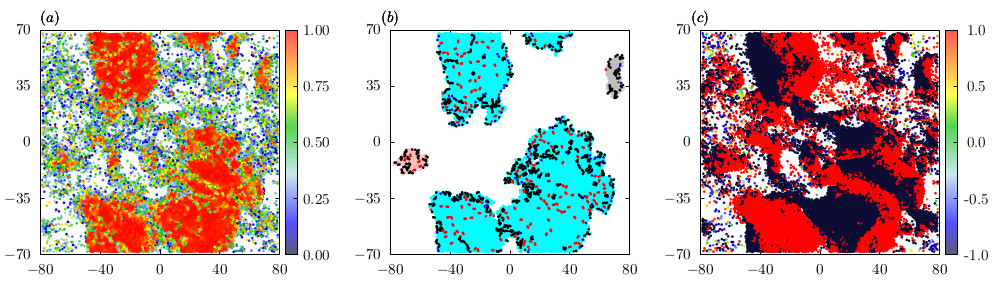 Figure 1
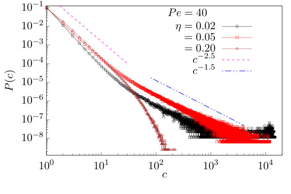 Figure 2
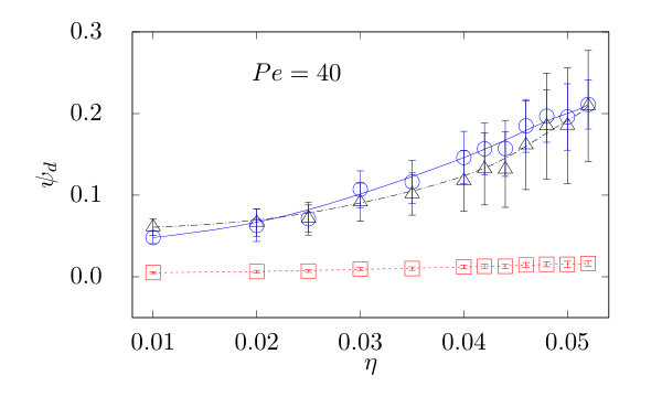 Figure 3
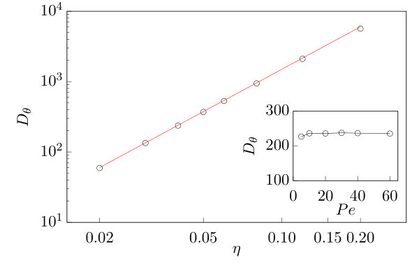 Figure 4
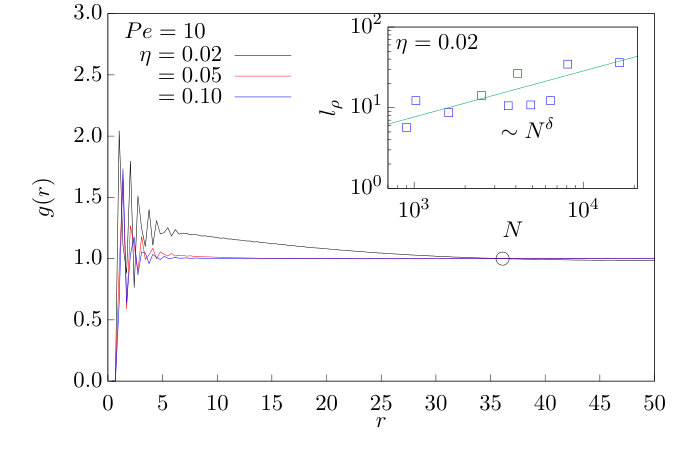 Figure 5
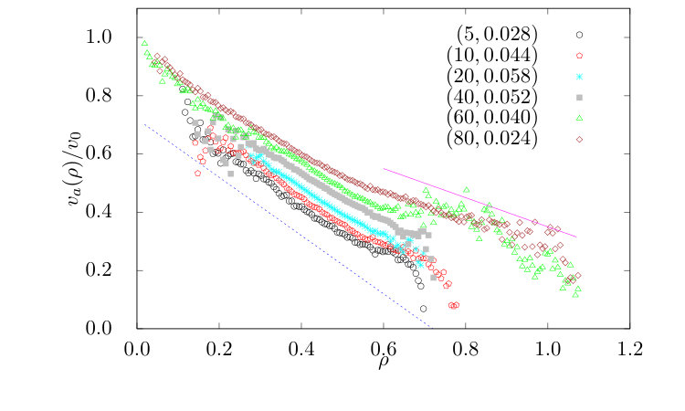 Figure 6
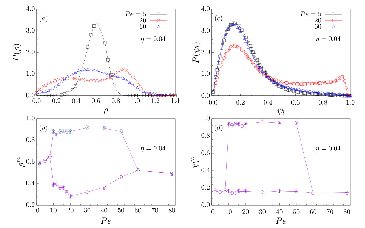 Figure 7
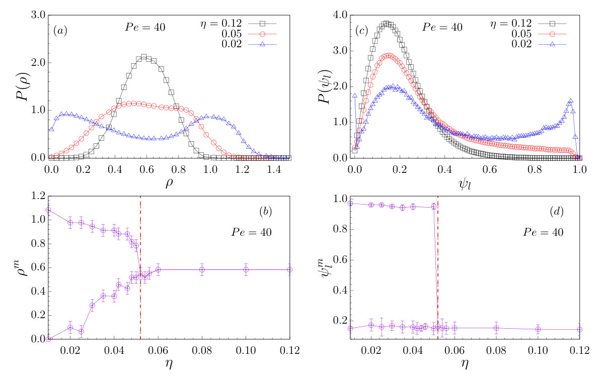 Figure 8
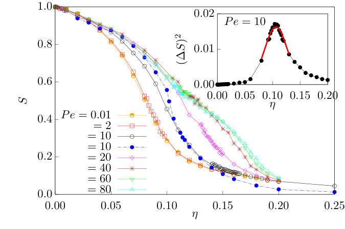 Figure 9
 Figure 10
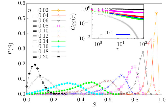 Figure 11
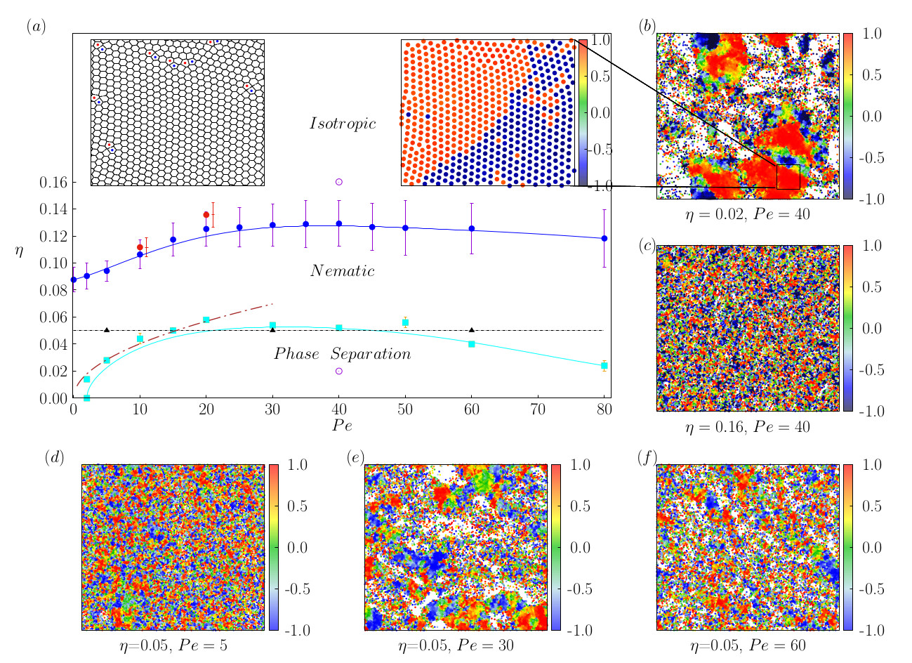 Figure 12
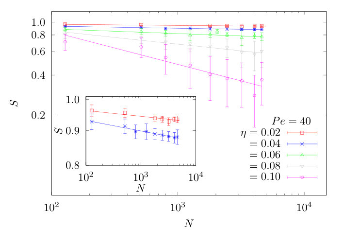 Figure 13
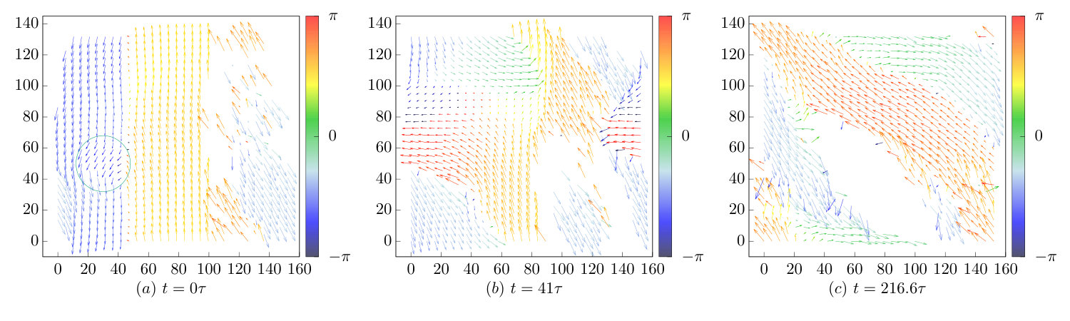 Figure 14
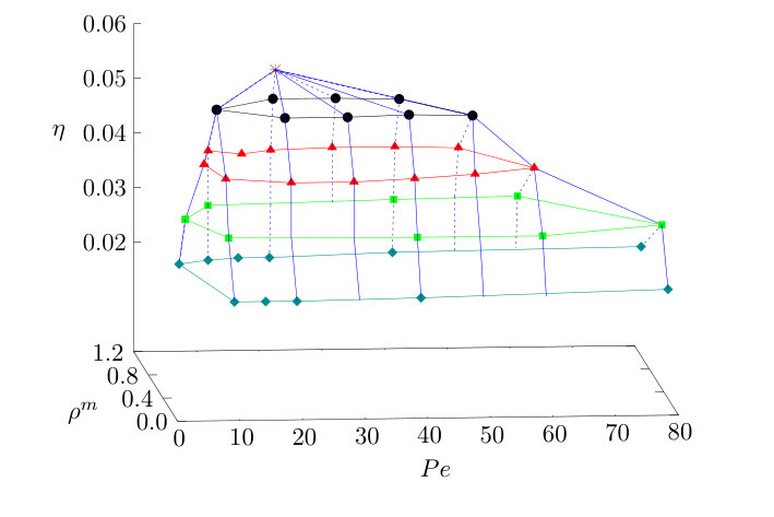 Figure 15
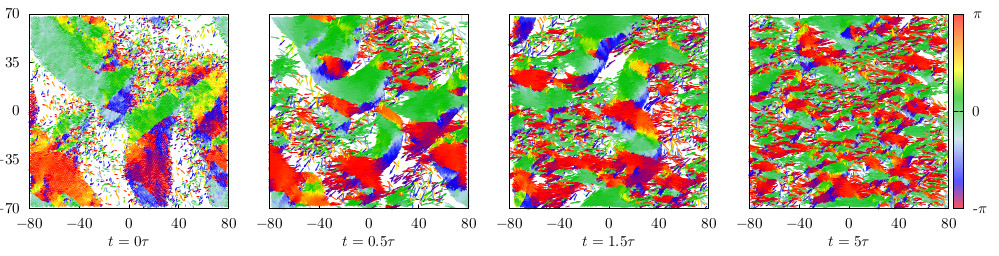 Figure 16
Peer Reviews
No public reviews on file for this paper yet. If you reviewed it on a platform where reviews are public (OpenReview, ICLR, NeurIPS, ICML), you can paste yours below so the community can read it here.
Videos
No videos yet. Explain this paper in a talk, walkthrough, or lecture? Add one.
Re-entrant phase separation in nematically aligning active polar particles
Biplab Bhattacherjee
Institute of Physics, Sachivalaya Marg, Bhubaneswar 751005, India.
Debasish Chaudhuri
Institute of Physics, Sachivalaya Marg, Bhubaneswar 751005, India.
Homi Bhaba National Institute, Anushaktigar, Mumbai 400094, India.
Abstract
We present a numerical study of the phase behavior of repulsively interacting active polar particles that align their active velocities nematically. The amplitude of the active velocity, and the noise in its orientational alignment control the active nature of the system. At high values of orientational noise, the structural fluid undergoes a continuous nematic-isotropic transition in active orientation. This transition is well separated from an active phase separation, characterized by the formation of high density hexatic clusters, observed at lower noise strengths. With increasing activity, the system undergoes a re-entrant fluid- phase separation- fluid transition. The phase coexistence at low activity can be understood in terms of motility induced phase separation. In contrast, the re-melting of hexatic clusters, and the collective motion at low orientational noise are dominated by flocking behavior. At high activity, sliding and jamming of polar sub-clusters, formation of grain boundaries, lane formation, and subsequent fragmentation of the polar patches mediate remelting.
pacs:
89.75.Fb, 05.65.+b
I Introduction
Active particles transduce stored or ambient energy into motion, generating non-equilibrium drive from the smallest scales of a system Marchetti2013 ; Romanczuk2012 ; Vicsek2012 . Examples in biology range from molecular motors, cytoskeleton, cells, tissues Schliwa2003 ; Alberts2007 ; Howarda ; Surrey2001 ; Schaller2010 , bacterial suspension Cates2012 ; Sokolov2007 to ant trails, bird flocks, animal groups and human crowd Toner2005 ; Ballerini2008 ; Couzin2007 ; Couzin2003 ; Katz2011 ; Attanasi2014 ; Helbing1997 ; Helbing2000 . In nonliving matter, examples include colloidal Janus particles Zottl2016 , and vibrated asymmetric granular matter Weber2013 . The seminal model by Vicsek, and its subsequent extensions Vicsek1995 ; Chate2006 ; Chate2008 ; Vicsek2012 , considered active point particles that orient the direction of their active velocity ferromagnetically, i.e., parallel to that of their neighbours. The collective properties of active particles depend only on a few microscopic details. The self propulsion can be polar Vicsek1995 ; Gregoire2004 or apolar Chate2006 ; Gruler1999 . The direction of propulsion may align parallel to or in a nematic manner with the neighboring particles Vicsek1995 ; Ginelli2010 . The alignment may arise from hydrodynamic coupling Sokolov2007 ; Katz2011 , visual cues Nagy2010 ; Ballerini2008 , or direct collision between extended objects Narayan2007 ; Peruani2006 ; Weber2013 ; Weitz2015 ; Shi2018 ; Grossman2019 . With increasing tendency of alignment and activity, the coupling of velocity fluctuations with density lead to flocking, collective motion, and giant number fluctuations Toner1995 ; Toner1998 ; Narayan2007 ; Dey2012 ; Gregoire2004 ; Peruani2011b ; Solon2013 ; Peruani2013 .
Another important aspect in the emergent phase behavior of active particles is the impact of volume exclusion. Its interplay with activity is most extensively studied in active Brownian particles (ABP) Fily2012 ; Redner2013 ; Solon2015 ; Stenhammar2013 ; Cates2015 . In ABPs the orientation of self propulsion of each particle undergoes Brownian rotation, independent of others. This persistent motion suppresses the change in velocity direction after collision between ABPs, unlike in elastic scattering. The resultant slow-down generates a positive feedback effect allowing accumulation of more particles to form clusters, eventually leading to a motility induce phase separation (MIPS) Cates2015 . The high density clusters could be in either a hexatic or solid phase, determined by the amount of activity and mean density Digregorio2018 . It has been shown recently that at low activity, the equilibrium two stage defect mediated melting scenario of two-dimensional solid Kosterlitz1973 ; Halperin1978 ; Young1979 ; Kapfer2015 ; Bernard2011 ; Gasser2010 ; Thorneywork2017 persists, with the melting points shifting to higher densities with increasing activity Klamser2018 ; Digregorio2018 .
The two aspects of active alignment and exclusion have been combined in a number of recent studies analyzing the impact of volume exclusion on ferromagnetically aligning active polar particles Peruani2011b ; Weber2014 ; Martin-Gomez2018 ; Sese-Sansa2018 . The role of topological defects in the melting of such active solids was demonstrated Weber2014 . At lower densities, the system shows formation of micro or macro clusters, lanes and bands Martin-Gomez2018 . A recent experiment observed interrupted phase separation in active Janus colloids where impact of alignment and excluded volume are simultaneously present Linden2019 . Active granular disks with built-in asymmetry showed polar activity under external shaking. These disks repel each other in a circularly symmetric fashion, and their active velocities showed approximate nematic alignment Weber2013 . Active point particles with nematic alignment were known to undergo nematic to isotropic phase transition and associated clustering Ginelli2010 .
In this paper, we investigate the effect of volume exclusion on the collective properties of nematically aligning active polar particles. Using numerical simulations, we present a comprehensive study of the active orientational phase transition and spatial phase separation with changing values of the active velocity and orientational noise. We fix the mean density at a value that is slightly lesser than the equilibrium melting point. With reduction of alignment noise, the active fluid shows a continuous isotropic to nematic phase transition. However, across this transition, structurally, the system remains in a homogeneous fluid phase, unlike the point particles. With further reduction of the noise, the active particles undergo a phase separation showing coexistence of high density hexatic clusters and low density fluid. This emerges due to the interplay of activity and excluded volume interaction. At an intermediate noise, the system demonstrates a remarkable re-entrant transition from fluid - phase coexistence - fluid with increasing active velocity. We present the detailed phase diagram, supported by a comprehensive characterization of the respective phases and phase-transitions in this paper. As we show, the onset of clustering at low active velocities is like MIPS, mediated by an effective slowdown of particles with density. The remelting of these active hexatic clusters at higher active velocities takes place by formation of grain boundaries and fragmentation of local polar patches. The cluster size distribution changes qualitatively at the onset of the phase separation. The hexatic clusters display complex dynamics – from sliding stripes, to jamming, to formation of counter-propagating channels. A finite size scaling analysis shows the robustness of the clustering transition, the mean cluster size remains a finite fraction of the overall system size even in the largest systems.
In Section II, we describe the model and simulation details. We present the complete phase diagram and the details of the phase transitions in Section III. Finally we conclude in Section IV presenting a summary and outlook.
II Model
We consider a two-dimensional system of active polar particles in a volume , performing active Brownian motion with a self-propulsion speed , in direction for the -th particle, where denotes the angle subtends with the -axis. The positional evolution of the -th particle is described by an overdamped Langevin equation
[TABLE]
where, is the mobility, is a Gaussian white noise with and so that , , is the repulsive force between particles given by the WCA potential Weeks1971
[TABLE]
where, is the inter-particle separation. We assume a nematic alignment of the polar orientation of the -th particle with its neighbors. It aligns (anti-) parallel to the local mean active orientation, if the relative angle between the two orientations is (obtuse) acute. We use the evolution Ginelli2010 ,
[TABLE]
The alignment gets randomized by the orientational noise that follows uniform distribution between with the noise strength .
The unit of length, energy, and time are set by , , and , respectively. The activity of the particles is controlled by a dimensionless Péclet number , and the noise strength . The numerical simulation is performed using Euler integration. We use integration time step for , and a smaller time-step for higher , to avoid inter-particle overlap.
In the absence of activity, the two-dimensional solid is expected to display a solid- hexatic- liquid equilibrium phase-transition Bernard2011 ; Kapfer2015 ; Kosterlitz1973 ; Halperin1978 ; Young1979 , with the solid melting point at the dimensionless density . We present results for , a density slightly below the equilibrium melting point. At this density, the excluded volume interaction plays an important role, while not dominating over activity.
III Phase transition
In this section, we present a detailed phase diagram, and extensive discussion of the corresponding phase transitions.
III.1 Phase diagram
Fig.1() shows the phase diagram in the - plane, identifying the isotropic, and the nematic fluid, and the region of active phase separation. With decreasing , the active orientations of isotropic fluid gets aligned in the nematic fashion, captured by the time-averaged scalar order parameter , where the mean nematic order of a given configuration is . The increasing convection of orientational information with increasing , requires a larger to destroy the nematic order. However, due to the volume exclusion, the range over which the nematic alignment may get extended due to convection is restricted at a given density. Thus the isotropic- nematic phase boundary shows an initial increase with before eventual saturation (Fig.1() ). The transition points denoted by the filled blue circles in Fig.1() are evaluated using particles. They are identified by the maximum of fluctuations in the order parameter . For comparison, we performed simulations for a larger system of particles at and . The red filled circles show the isotropic-nematic transition points corresponding to this system size. They compare well with particle results, within error bars. The determination of the transition points and the corresponding error bars are discussed in detail in Sec. III.2.
At further lower , the active system undergoes phase separation between a nematic fluid and denser hexatic clusters. The phase coexistence is captured by the bimodal distribution function of the local density , and the amplitude of the local hexatic bond-orientational order , where denotes the number of particles in a coarse-grained volume around . The bond-orientational order associated with the -th particle is defined as Mickel2013 ; Steinhardt1983 , where, is the angle subtended by the bond between the -th particle and its -th Voronoi neighbor on the positive -axis; is the length of the Voronoi edge corresponding to the -th neighbor, and where is the total number of Voronoi topological neighbors. The solid line denotes the onset of phase coexistence of the nematic fluid and hexatic clusters. The non-monotonic variation of this boundary as a function of indicates a re-entrant transition. For example, keeping the orientational noise strength fixed at , change in from to leads a nematic fluid to the hexatic- nematic fluid phase coexistence. The hexatic clusters remelt into a homogeneous nematic fluid by increasing further to . The dashed line shown at the phase boundary is an estimate obtained using the argument of MIPS, as outlined later in Sec.III.3. The clusters in the rest of the phase coexistence regime are dominated by alignment and flocking. Before going into the quantitative analysis, we illustrate the local phase behavior in terms of system configurations and local hexatic order.
Fig.1()-() show typical instantaneous configurations of particles shaded by colors denoting the projection , of their individual hexatic orientations to the instantaneous system averaged bond-orientational order . is bounded between and . Fig.1() shows a typical configuration in the two phase regime. The high density clusters of particles are observable as contiguous colored patches. The large red patches identify regions with local bond orientational order aligned along the mean instantaneous hexatic order. On the other hand, the blue patches denote the regions where local bond orientational orders are anti-parallel to that of the mean hexatic order. A magnified portion of one such high density cluster is shown in the upper right inset in Fig.1(). It shows local formation of solid-like triangular lattice structure. This region of high six-fold bond orientational order is a jammed state of two sets of active particles with opposite polarity, denoted by red and blue colors in this figure. In the upper left inset of Fig.1(), we show the same configuration in terms of Voronoi tessellation, color coding the disclinations where the particles do not have six Voronoi neighbours, denoting particles with five neighbors in blue and that with seven neighbors in red. In a pure triangular lattice, all particles have six neighbors. The presence of bound disclination pairs, well-separated from each other, identify free dislocations, a characteristic of the hexatic phase. Fig.1() shows a typical configuration in the isotropic fluid phase. The two phase points at which configurations Fig.1(),() are plotted are denoted by pink circles in the phase diagram Fig.1(). The black dashed line in the phase diagram Fig.1() follows a remelting transition. Typical configurations corresponding to the three points denoted by in Fig.1() are presented in Fig.1()-(), showing significant hexatic clustering in Fig.1(). The details of these phase transitions are quantified in the following.
III.2 Isotropic Nematic Transition
The nematic-isotropic transition is quantified by following the reduction of the nematic scalar order parameter with the increase in the orientational noise strength . This is shown for seven different values in Fig.2, using a system of particles. The fluctuation of the order parameter shows a pronounced maximum at the transition point . A representative behavior is shown in the inset of Fig.2 for . This maximum is identified as the transition point. To determine the exact location of the maximum and its standard deviation , we use a Gaussian fitting around the maximum (red solid line in the inset of Fig.2). These constitute the nematic-isotropic phase transition points and their error-bars plotted in Fig.1(). With increasing system size, the transition becomes sharper, however, the transition point remains within the error bar. One data set for a larger system of particles at is shown using the filled blue circles in Fig.2. The observed transition is between a quasi-long ranged ordered (QLRO) nematic phase to a disordered isotropic phase. The QLRO within the nematic phase is illustrated in Appendix-A in terms of an algebraic decay of the scalar order parameter with system size. A further discussion on the nature of curves, and their data-collapse in an intermediate regime are presented in Appendix-B.
The nature of the nematic-isotropic phase transition is further qualified using the probability distribution of the scalar order parameter, , across the transition. At a given activity, with increasing the probablity distribution remains unimodal, only the peak position shifts from to values close to (Fig. 3). This unimodal nature of the distribution functions signifies the absence of any metastable phase on the other side of the transition, a characteristic of continuous transitions. The distributions broaden near the phase transition point capturing the enhanced fluctuations.
The continuous nature of the transition is further characterized using the two-point correlation of the normalized nematic order parameter . The correlations are plotted for different at in the inset in Fig. 3. Within the QLRO nematic phase, the correlations decay as power law , with the value of the exponent increasing with . At the transition point the exponent , in approximate agreement with the prediction of equilibrium Kosterlitz-Thouless transition Kosterlitz1973 .
Across the nematic-isotropic transition, the volume exclusion maintains a homogeneous density distribution. This behavior is quite unlike that observed for point particles, where increased orientational disorder leads to density inhomogeneity resulting in clustering, and band formation Ginelli2010 . This remains the zero density or vanishing exclusion interaction limit of our model. At further smaller , enhanced alignment reduces orientational diffusion, thereby, increasing persistence. As a result, as we show in the following section, the interplay of activity and volume exclusion leads to phase separation.
III.3 Phase separation
The structural order in the coexisting phases are analyzed using a system of particles in a volume of with and fixing the dimensionless density to . The phase behavior is studied varying and values. At , the system undergoes phase separation with increasing . We characterize the phase coexistence using the density distribution function and the distribution of local hexatic order , where are calculated over local coarse-grained volumes of around . The system is relaxed up to , before analyses are performed using configurations saved in intervals of obtained from simulations over further .
III.3.1 Re-entrant phase separation with
In the regime of small orientational noise , a re-entrant phase-separation is observed with increasing . A detailed characterization is presented in Fig.4 for a fixed . At low activities, e.g., , exhibits a single maximum at the mean density corresponding to the homogeneous fluid (see Fig.4() ). With increasing , initially the distribution broadens, capturing the increased fluctuations in density. As the activity is further increased to , clusters form, and the system phase separates into high and low density regions.
The phase separation is most pronounced at . The phase separation persists up to . As activity is increased further to , the high density clusters get destabilized and the bimodality disappears identifying remelting. The new unimodal distribution is significantly broad with respect to the fluid before the onset of phase separation at small . It shows a shallow peak near (Fig.4() ). This is due to the larger density fluctuations associated with the stronger activity. The peak position(s) of the local density distributions for are plotted as a function of in Fig.4(). This clearly demonstrates phase coexistence over an intermediate regime of , between to .
Associated with the clustering, a local hexatic order emerges. Three representative probability distributions at values corresponding to the two homogeneous phases and the phase coexistence region, are shown in Fig.4(). At the distributions show a single maximum at a low hexatic order . At intermediate values, e.g., , a bimodality in is observed, showing emergence of a new large peak near , associated with the emergence of the high density hexatic clusters. However, even within the phase coexistence region, , the larger peaks of the distributions remain at a small value, reflecting the fact that the homogeneous fluid covers the larger spatial fraction of the system. The peak positions of the probability distributions are plotted in Fig.4(). This again captures the re-entrant phase separation, as in Fig.4(). With increasing , the system shows a re-entrant transition from a single fluid to a fluid-hexatic coexistence that finally returns to a single fluid.
III.3.2 Phase separation with
To demonstrate the dependence of the phase separation on the strength of orientational fluctuations , we consider the system at a sufficiently high activity and vary . As we have seen above, at this activity the system remains phase separated at . In Fig.5() we show the variation of with . At low (, blue up triangles), the system remains phase separated, captured by the bimodality of . With increasing , the peaks in the distribution slowly come together and merge at (red circles). For larger , the density distribution remains unimodal (e.g., , black squares) with the peak at the mean density , signifying a homogeneous fluid phase. The peak positions of are plotted against in Fig.5(). This shows how the coexistence lines merge together as a function of at a critical point. This behavior is similar to the merger of liquid-gas coexistence lines as the critical temperature is approached from below. The detailed properties of such a critical point has been explored for the ABPs recently Siebert2018 , and remains to be studied in the current context in future. The distributions of the local hexatic order show pronounced multi-modality at the phase coexistence. The peak near captures the significantly large hexatic order of the active clusters. The other peak near signifies the coexisting homogenoeus fluid. In addition, we observe a peak at , which corresponds to the voids generated at the cost of clustering. The non-zero peaks of are plotted against in Fig.5(), recapturing the loss of phase coexistence with increasing , as in Fig.5().
Using the above analysis it is possible to construct a combined phase- coexistence diagram in the plane as is shown in Fig.6. The values denote the binodals extracted from the peaks of the probability distribution of the local density. The apex of the plot at large denotes the critical point below which phase coexistence becomes possible. The lines indicate the boundary of the onset of phase coexistence. As is clear from the plot, the coexisting densities separate out more strongly at lower . At a given , after the onset of active phase separation appears at a low , coexisting densities first separate out to finally merge as is increased. At lower , large activity supports formation of flocks. As a result this merger happens at a larger . Moreover, lowering of reduces the orientational diffusion supporting MIPS at small , thereby reducing the value at which phase separation appears. The flocking and MIPS mechanisms are discussed further in the following section.
III.3.3 Cluster formation
In the absence of alignment, volume exclusion induces slow down of active motion with increasing local density generating a positive feedback mechanism that mediates MIPS. However, the clustering we observe is deep within an orientationally ordered nematic phase. This raises the question whether the MIPS- like mechanism still plays any role in clustering, or the phase coexistence is due to the onset of flocking related to orientational fluctuations. It was argued before that alignment for polar disks reduces rotational diffusion, and thereby may favor MIPS Martin-Gomez2018 ; Sese-Sansa2018 . On the other hand, steric alignment of self propelled rods beyond an asymmetry parameter produces destabilizing torques to break MIPS clusters Grossman2019 ; Shi2018 ; Weitz2015 . We note that, for our self propelled disks in the nematic phase with antiparallel active orientations, crowding effects may slow down the propulsion speed. In fact, as we show below, this is the dominant mechanism of clustering in the small regime.
Here we compute the self-propulsion speed reduced by the inter-particle repulsion at a local density . We proceed by calculating the coarse- grained quantity in cells of volume having particles Sese-Sansa2018 , such that the instantaneous density is . Within the MIPS paradigm, it is expected that where depends on , a stall time at collision, and a scattering cross-section Stenhammar2013 . Fig.7 shows the variation of along the phase separation boundary. In the small regime, between to , decreases linearly with with a single slope , in agreement with the MIPS expectation. However, at higher , the behavior starts to get dominated by flocking, shown by the slow down of the decay of at higher . Note the cross-over to a second slope at large for . This happens as a cluster starts to get an effective polar alignment such that the active velocities of particles do not completely block each other. Similar cross-overs have been observed earlier for ferromagnetically aligning ABPs Sese-Sansa2018 .
At small , colliding particles slow down as in MIPS. The size of a hexatic cluster is maintained by the absorption of particles from the surrounding fluid having density , with a rate and evaporation from the cluster surface due to reorientation of the direction of self-propulsion with a rate , where denotes the total number of particles leaving the cluster in each escape Redner2013 . The orientational relaxation is controlled by the noise strength , such that the related rotational diffusion constant (see Appendix-C). The mean density of the system in the phase coexistence regime can be expressed as , where () denotes the mean density of the hexatic (liquid) fraction, and denotes the amount of hexatic fraction. At the onset of phase coexistence, and . Thus, equating and setting , we get . This leads to the condition . Using we obtain the prediction for MIPS- like phase boundary , plotted in the phase diagram Fig.1(). This captures the behavior of the low boundary for the onset of active phase separation.
To illustrate the melting process of hexatic clusters at high , in Fig.8, we show the evolution of a steady state configuration after quench from within the phase coexistence regime at and to , an activity beyond the remelting boundary. The plots show velocity orientation (color code) and speed (arrow) of particles, e.g., right moving particles (orientation [math]) are denoted by green and the left moving ones by red (orientation ). If counter moving polar patches do not block each other, they slide past. In other places, e.g., in the largest cluster in the upper- left corner at the initial configuration (Fig.8), a left moving patch creates channel and squeezes through the majority right moving particles. The polar patches eventually detach, destabilizing the big clusters to smaller clusters. Similar ejection of polar clusters were observed before in self propelled rods Weitz2015 . The ejection process continues to finally melt the hexatic clusters, e.g., see the last configuration after a time lapse of in Fig.8. The detailed dynamics can be observed in the movie added in the supplemental material 111The video shows the time evolution of the local density and velocity fields over after a quench from to at . The color code in the video follows that in Fig.8..
III.4 Topological defects
In this section we investigate the role of the topological defects in the melting of the active hexatic clusters. We define the coordination number of each particle as the number of Voronoi neighbours it has. The particles constitute the topological defects. Within hexatic clusters, particles with and stay as bound pairs. Such bound pairs, well separated from each other, identify the presence of dislocations in hexatic. For example, see the upper left inset in Fig.1() displaying several bound pairs in a portion of a hexatic cluster of the active system. Unbinding of such pairs, generate free disclinations. As we show, interconnected chains of defects form grain boundaries, held by local polar patches of the hexatic clusters.
We analyze the variation of the fraction of particles belonging to different defect types within the hexatic clusters, with increasing at Qi2014 . A typical configuration at is shown in Fig.9. In Fig.9() we display the hexatic order associated with all the particles . The large clusters have an overall large hexatic order . The local drops in the values of within the large clusters are associated with formation of topological defects. In Fig.9() we show the three different defect types separately – dislocations (red points), disclinations (blue points) and grain boundaries (string of black points) within the three largest clusters colored with cyan (largest cluster), grey (2nd largest cluster) and pink (3rd largest cluster). To understand the localization of the grain boundaries, we display the projection of the local polar orientation of the particles onto the orientation of instantaneous overall nematic order in Fig.9(). A comparison between Fig.9() with () shows that the grain boundaries appear at the interface of anti-parallel polar patches of activity. At high activity, such as , the opposing active push from these neighboring polar regions leads to the formation of the grain boundaries within the clusters.
To quantify the behaviour of the topological defects across the melting transition, we compute the fraction of particles associated with the dislocations, grain boundaries and disclinations within the largest cluster of a given configuration. The averaging is performed over more than well separated configurations in the steady state. In Fig.10 we show the variation of these three average quantities with increasing , at . In the active clusters, all the disclinations are thrown out to the hexatic- fluid interfaces. The fraction of the disclination within the hexatic cluster, thus, remains largely unchanged. The fraction of dislocations increases with , as well as the fraction of grain boundaries. Note that the dislocations characterize hexatic phase, and do not destabilize it. Thus the melting of the active hexatic at large is mediated by grain boundary formation along the interface of oppositely aligned polar patches within a cluster.
III.5 Cluster size and dynamics
As has been mentioned before, the coexistence at the active phase separation is characterized by the presence of large correlated clusters. They are identified using a clustering algorithm, defining particles within a separation to be part of a single cluster Allen1989 . The number of particles belonging to a cluster determines the cluster size . Three typical steady state cluster size distributions in the homogeneous fluid phase and at the active phase coexistence are shown in Fig.11.
The distribution of small clusters are approximately independent of the phase, and the weight decays as . The decay of the distribution for large clusters, on the other hand, changes qualitatively with the change in phase. In the homogeneous fluid phase, it decays exponentially. In contrast, in the regime of phase separation, the tail of the distribution shows a power law decay . This appears in addition to a small but approximately uniform weight associated with the largest clusters. The change of the tail of the cluster size distribution from exponential decay to a power law is qualitatively similar to that observed in the conserved mass aggregation model (CMAM) Majumdar1998 , however, the exponents in our case differ significantly. Moreover, for the largest clusters structural ordering competes with ejection of polar fractions, not allowing stabilization of infinite-aggregates, unlike in the CMAM.
A measure of the spatial extension of the clusters is the correlation length obtained from the two point density correlation function . In Fig.12 the variation of is shown in the fluid and the phase coexistence region. The typical correlation length, , is estimated as the value of the separation beyond which the correlation decays to . As is shown in Fig.12, in the regime of phase separation () one gets a large () corresponding to the large extension of the clusters. However, in the homogeneous fluid phase the correlation length becomes small (). If the appearance of phase separation is not a finite size effect, the cluster size should remain a finite fraction of the system size , in the thermodynamic limit of infinite . To test this we perform a system size scaling. As we show in the inset of Fig.12, indeed, the ratio does not decrease with system size .
The collective motion is dominated by flock- like behavior at large as well as small , at which alignment dominates. This consists of (i) structurally ordered stripes sliding past each other, (ii) jamming of polar clusters, (iii) which eventually break via formation of counter-propagating channels. The behaviors are shown in Fig.13()-() with the help of local vector fields identifying the orientations and amplitudes of the locally coarse grained velocity of particles. The coarse- graining is performed over cells of size , and the velocity fields are calculated from displacements obtained over . The orientations of velocity are further highlighted by color codes explained in the figure. The snapshots are shown at three different well separated time instances in the steady state, deep inside the phase coexistence regime. For the ease of illustration, we have chosen and , as the clusters at such a low are system spanning in extension and have long life-times.
In Fig.13() we plot the first steady-state snapshot of local velocity fields. It shows two large counter propagating clusters that glide past each other, in the up and down directions (). The velocity field at the interface of the two clusters vanishes, before changing direction. With time, the velocity field from one domain may penetrate the other due to dynamical fluctuations along the interface. In Fig.13(), such events are identified by a bulge of vectors marked within a circle. This generates instability towards the formation of lanes. At a later time, , as is shown in Fig.13(), particles in this region starts to flow leftward (direction ). They create path for other particles to trickle along. As time progresses, this local trickling takes the form of a stream of particles forming counter propagating lanes, as is shown in Fig.13() at . The crossovers between these different regimes happen faster at higher and .
IV Discussion
We have studied the combined effect of volume exclusion and nematic alignment on collective behavior of active polar particles. Using numerical simulations, we have presented a phase diagram encapsulating the structural and orientational transitions with changing activity and noise . In the equilibrium limit of vanishing activity our system behaves as a high density fluid. On the other hand, the limit of vanishing interaction reduces it to the nematically aligning point particles Ginelli2010 . The nematic-isotropic transition in activity obtained by increasing does not change the homogeneous nature of the fluid phase of the excluded volume particles. This behavior is in striking contrast to the properties observed for point particles Ginelli2010 , where the nematic-isotropic transition was accompanied by phase separation. The volume exclusion in the current model, in addition to a significant rotational diffusivity, , even at the nematic-isotropic transition, suppresses such fluctuations.
However, we do find clustering transition in our system, but at a lower strength of associated with larger persistence, . As we have shown, the competition of persistence and volume exclusion led to a kinetic slowdown with density. This provided a MIPS mechanism towards phase separation at small . The nematic fluid undergoes a transition from the homogeneous phase to an active phase separation characterized by the formation of high density hexatic clusters. We found a re-entrant fluid- phase coexistence- fluid transition with increasing . At the small regime, volume exclusion dominates – the formation of clusters is mediated by the slow-down of colliding particles providing a positive feedback, as in MIPS. The phase boundary in this regime follows a form , that could be motivated using the MIPS phenomenology.
With increasing , the opposing push from the counter propagating polar sub-regions of a nematic cluster leads to formation of grain boundaries. Once the active push gets large enough, opposing polar regions squeeze past each other forming lanes. At higher , the clusters eject polar patches that form co-moving flocks. At high enough , this breaking and ejection of polar patches continue to dissolve larger clusters into smaller ones, finally leading to remelting. As in the high regime, at the lowest orientational noise strengths, alignment dominates leading to flock- like collective motion that consists of sliding clusters, jamming, and lane formation.
An experiment on active colloidal disks, recently, examined the combined impact of volume exclusion and alignment in the phase separation kinetics at high activity Linden2019 . Similar experiments, may potentially verify our predictions. A coarse grained hydrodynamic description combining active alignment and density dependent slowdown remains to be developed, and may provide further insight into the phase transitions of such systems.
Acknowledgements
The simulations were performed on SAMKHYA, the high performance computing facility at IOP, Bhubaneswar. DC thanks ICTS-TIFR, Bangalore for an associateship, and SERB, India, for financial support through grant number EMR/2016/001454.
Appendix A Quasi long range order
Here we demonstrate the nature of the nemtaic order before the nematic-isotropic transition. To this end, we perform a system size analysis by calculating the scalar order parameter for system sizes to , at a fixed , and varying (Fig.14). With increasing , we find an algebraic decay , where both and the exponent depend on . Even at the smallest , the algebraic decay of the order parameter with system size is evident (see inset of Fig.14). This is a signature of the quasi- long ranged order (QLRO) of the active nematic phase mentioned in Sec.III.2. The exponent increases with .
Appendix B Scaling of the - curves
We identify three different regimes, depending on how the function behaves at different (Fig.2). For , the curves fall on top of each other implying that a minimum activity is required for the system to show effects of in the macroscopic scale. This vanishes with increase in system size(data not shown). Increase in , allows a single particle to cover larger space, nematically aligning with larger number of particles over a span of time. Thus a larger orientational noise is required to destabilize the nematic phase, increasing the transition noise with . However, for a given density, there is a limit up to which can suppress the nematic to isotropic transition. This limit is decided by the available free space, determined by the mean density. For , again, the curves fall on top of each other, making independent of . In between and , the variations of with show data collapse when plotted against (Fig.15). Within this restricted window of activity, we find a dependence of transition point with that shows an approximate scaling form (inset in Fig.15).
Appendix C Orientational relaxation
In the presence of the nematic alignment, the active orientation of the particles undergo orientational relaxation controlled by the noise of strength . In Fig.16 we show that the orientational diffusion constant increases as , and remains essentially unchanged with variation of .
The reference list from the paper itself. Each links out to its DOI / PubMed record.
- 1(1) M. C. Marchetti, J. F. Joanny, S. Ramaswamy, T. B. Liverpool, J. Prost, M. Rao, and R. A. Simha, Rev. Mod. Phys. 85 , 1143 (2013).
- 2(2) P. Romanczuk, M. Bär, W. Ebeling, B. Lindner, and L. Schimansky-Geier, Eur. Phys. J. Spec. Top. 202 , 1 (2012).
- 3(3) T. Vicsek and A. Zafeiris, Phys. Rep. 517 , 71 (2012).
- 4(4) M. Schliwa and G. Woehlke, Nature 422 , 759 (2003).
- 5(5) B. Alberts, A. Johnson, J. Lewis, K. R. Martin Raff, and P. Walter, Molecular Biology of the Cell , 6th ed. (Garland Science, New York, 2007).
- 6(6) J. Howard, Mechanics of Motor Proteins and the Cytoskeleton (Sinauer, Sunderland, MA, 2001).
- 7(7) T. Surrey, F. Nédélec, S. Leibler, and E. Karsenti, Science 292 , 1167 (2001).
- 8(8) V. Schaller, C. Weber, C. Semmrich, E. Frey, and A. R. Bausch, Nature 467 , 73 (2010).