Relation Between Solutions of the Schr\"odinger Equation with Transitioning Resonance Solutions of the Gravitational Three-Body Problem
Edward Belbruno

TL;DR
This paper demonstrates a link between classical gravitational three-body resonance solutions and quantum-like Schr"odinger equation solutions, showing how macroscopic resonance transitions mirror quantum energy state changes.
Contribution
It introduces a novel approach connecting celestial three-body resonances with quantum mechanics through a modified Schr"odinger equation.
Findings
Resonance solutions transition via weak capture in the three-body problem.
Quantized wave solutions correspond to energy state transitions.
Classical resonance dynamics model quantum energy state changes.
Abstract
It is shown that a class of approximate resonance solutions in the three-body problem under the Newtonian gravitational force are equivalent to quantized solutions of a modified Schr\"odinger equation for a wide range of masses that transition between energy states. In the macroscopic scale, the resonance solutions are shown to transition from one resonance type to another through weak capture at one of the bodies, while in the Schr\"odinger equation, one obtains quantized wave solutions transitioning between different energies. The resonance transition dynamics provides a classical model of a particle moving between different energy states in the Schr\"odinger equation. This methodology provides a connection between celestial and quantum mechanics.
Click any figure to enlarge with its caption.
 Figure 1
 Figure 140
 Figure 150
 Figure 180
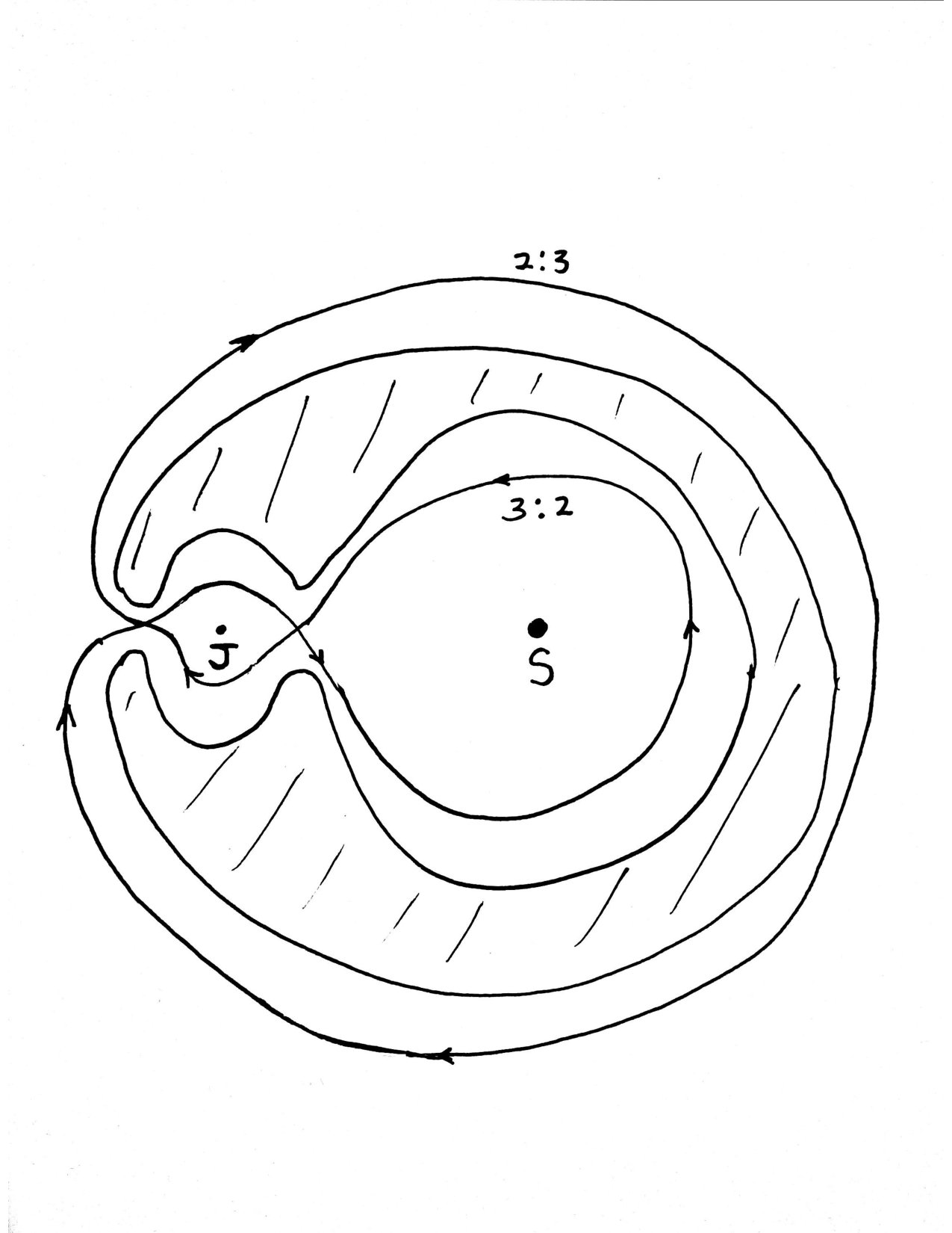 Figure 190
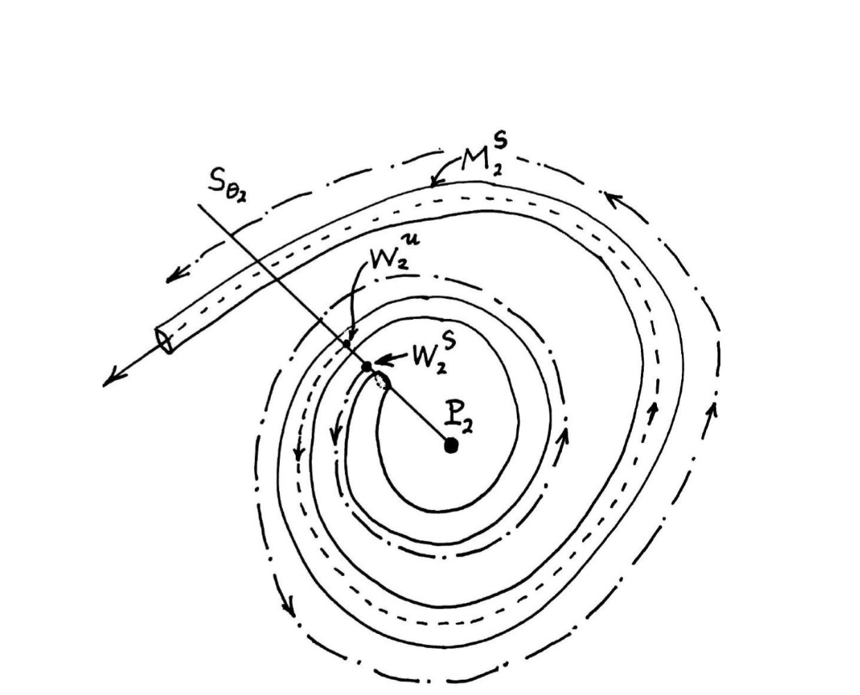 Figure 2
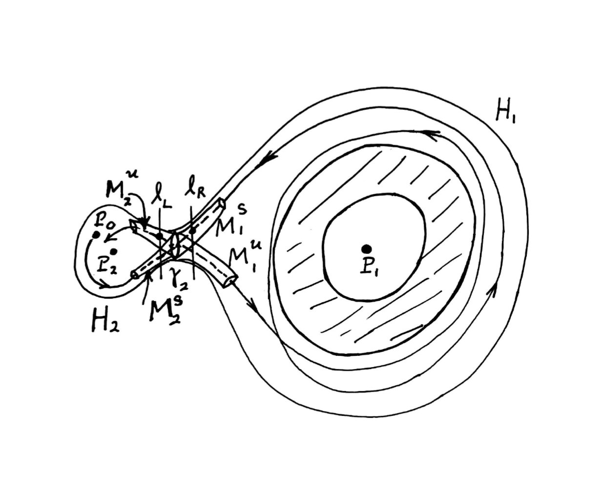 Figure 3
Peer Reviews
No public reviews on file for this paper yet. If you reviewed it on a platform where reviews are public (OpenReview, ICLR, NeurIPS, ICML), you can paste yours below so the community can read it here.
Videos
No videos yet. Explain this paper in a talk, walkthrough, or lecture? Add one.
Taxonomy
TopicsQuantum Mechanics and Applications · Cold Atom Physics and Bose-Einstein Condensates
Relation Between Solutions of the Schrödinger Equation with Transitioning Resonance Solutions of the Gravitational Three-Body Problem
Edward Belbruno
Department of Mathematics, Yeshiva University, New York, NY, USA; Department of Astrophysical Sciences, Princeton University, Princeton, NJ, USA
Abstract
It is shown that a class of approximate resonance solutions in the three-body problem under the Newtonian gravitational force are equivalent to quantized solutions of a modified Schrödinger equation for a wide range of masses that transition between energy states. In the macroscopic scale, the resonance solutions are shown to transition from one resonance type to another through weak capture at one of the bodies, while in the Schrödinger equation, one obtains quantized wave solutions transitioning between different energies. The resonance transition dynamics provides a classical model of a particle moving between different energy states in the Schrödinger equation. This methodology provides a connection between celestial and quantum mechanics.
pacs:
05.45-a, 03.65.-w, 04.60.-m, 45.50.Pk
1 Introduction
The purpose of this paper is to describe a mechanism to globally model the solutions of a modified Schrödinger equation and how they transition between energy states, with a special set of approximate resonance solutions to the classical gravitational Newtonian three-body problem, for a wide range of masses. These resonance solutions transition from one resonance to another through the process of weak capture.
We consider a special version of the three-body problem that has proved to be useful in understanding the complexities of three-body motion, in the macroscopic scale, going back to Poincaré [1]. This is the circular restricted three body-problem, where the motion of one body, , is studied as it moves under the influence of the gravitational field of , assumed to move in mutual circular orbits of constant frequency . It is also assumed that the mass of , labeled , is negligible with respect to the masses of , labeled , respectively. In this paper, we will also assume that is much smaller than , . For example, in the case of planetary objects, one can take to be the Earth, Moon, respectively, and to be a rock. One can scale down , as well as the relative distances between the particles, until the quantum scale is reached where the pure gravitational modeling is no longer sufficient. When using a rotating coordinate system that rotates about the center of mass of with constant frequency , it is well known that Hamiltonian function for the motion of is time independent defining a conservative system (see Section 3 ).
For a general class of conservative systems, that includes, for example, the restricted three-body problem considered here, it is known that such systems can be associated to the Schrödinger equation. As is described in Lanczos [2], this can be done by computing the action function for the motion of , where is the position of . 111 is obtained as the integral of the Lagrangian function , over minimizing trajectories . is a solution of the Hamilton-Jacobi partial differential equation associated to the restricted three-body problem. The are orthogonal to the surface , for constant . In this sense, the iso- surfaces locally determine the trajectories , that is for having sufficiently small variation. On the other hand, it can be shown that is the phase of wave solutions to the Schrödinger equation. Thus, is a wave surface. Conversely, starting with the satisfying the Schrödinger equation, one obtains the Hamiltonian-Jacobi equation provided the Planck’s constant . This equivalence is local since in general can only be shown to locally exist as a solution to the Hamiltonian-Jacobi equation, which is the case for the three-body problem. For the full equivalence it is necessary that one restricts that is not realistic. More significantly, this equivalence does not determine the global behavior of the solutions and how they dynamically can model the transition of energy states for solutions of the Schrödinger equation.
This paper will use methods of dynamical systems to globally determine special resonance motions for that are shown to be equivalent to different energy states for a modified Schrödinger equation and where the transition between energy states is equivalent to the process of weak capture in the three-body problem described in this paper. This result does not require the restriction of Planck’s constant, and doesn’t use Planck’s constant in the modeling. The action function is not used. Due to the complexity of the motions described, it is seen that using the iso- surfaces to locally determine the global solutions would not seem feasible.
We describe a mechanism for the existence of a special family, , of approximate resonance motions of about , that transition from one resonance to another by the process of weak capture by . This is a temporary capture defined in Section 2. These motions are approximately elliptical with frequency . or equivalently , are functions of the time , where is approximately equal to the constant values , are positive integers. That is, the period of motion of is approximately synchronized with the circular motion of about , where in the time makes approximately revolutions about , makes revolutions about . The approximate resonance value of the frequency means that , for a small tolerance as time varies for restricted time spans, described in Section 2. When is moving on an approximate resonance orbit about , it will eventually move away from this orbit and become captured temporarily about , in weak capture. When escapes from this capture, it again moves about in another resonance elliptical orbit, with approximate resonance . This process repeats either indefinitely, or ends when, for example, escapes the -system. This also implies that the approximate two-body energy of about can only take on a discrete set of values, at each time , which are approximately constant defined by the resonances. This is stated as Result A in Section 2 and as Theorem A in Section 3. The properties and dynamics of weak capture, and weak escape, are described Section 3. Comets can perform such resonance transitions(see Sections 2 3).
A modified Schrödinger equation is defined for the motion of about , under the gravitational perturbation of . This is first considered in the case of macroscopic masses. It is given by,
[TABLE]
where is the Laplacian operator, is an averaged three-body gravitational potential, is the energy, and is the reduced mass for . is a function that depends on and , the gravitational constant. replaces , is Planck’s constant that is in the classical Schrödinger equation. In this case, for macroscopic values of the masses, since is not a wave, is used to determine the probability distribution function, , of locating near as a macroscopic body. We show in Section 4 that can only take on the following approximate quantized values,
[TABLE]
. As seen in Section 2, this implies that the frequency of takes a particularly simple form that is independent of any parameters. These frequencies have the approximate values, . is explicitly computed in Section 4. is shown to be exponentially decreasing as a function of the distance of from . The general solution, , of the modified Schrödinger equation is described in Result B in Section 2.
A main result of this paper is that the quantized energy values correspond to a subset, , of the resonance orbit family, , of about . This is listed as Result C in Section 2. This provides a global equivalence of the solutions of the modified Schrödinger equation with the transitioning resonance solutions of the the three-body problem.
As a final result, we show is that the solution, , for the location of for the modified Schrödinger equation for the macroscopic values of the masses, can be extended into the quantum-scale. This is summarized as Result D in Section 2. This gives a way to mathematically view the resonance motions in the quantum-scale, as an extension of the resonance solutions for macroscopic particles. Other models, such as the classical Schrödinger and Schrödinger-Newton equations are given in latter sections.
The results of this paper are described in detail and summarized in Section 2. This section contains the main findings of this paper. Additional details, derivations, and proofs are contained in Section 3 for weak capture and in Section 4 for the modified Schrödinger equation.
2 Summary of Results, Definitions and Assumptions
In this section we elaborate on the results described in the Introduction. The first set of results pertain to a family of resonance orbits about obtained from the three-body problem and the second set of results pertain to finding these orbits using a modified Schrödinger equation.
2.1 Resonance Orbits in the Three-Body Problem and Weak Capture
The motion of is defined for the circular restricted three-body problem described in the Introduction. It is sufficient to use the planar version of this model, without loss of generality for the purposes of this paper, where moves in the same plane of motion as that of the uniform circular motion of of constant frequency (see Section 3). The macroscopic masses satisfy, and the mass of is negligibly small so that does not gravitationally perturb , but perturb the motion of . We consider an inertial coordinate system, , whose origin is the center of mass of .
The differential equations for are given by the classical system
[TABLE]
where , , , () and
[TABLE]
where , , is the standard Euclidean norm. The mutual circular orbits of are given by , , with constant circular frequencies of , respectively. We have divided both sides of (3) by and then took the limit as . It is well known that the solutions of the circular restricted three-body problem for accurately model the motion of in the general three-body problem for circular initial conditions for , with kept positive and negligibly small.
It is noted that all solutions considered in this study will be in both and initial conditions, at an initial time . We refer to as smooth dependence. More exactly, this means that all derivatives of with respect to of all orders are continuous and all partial derivatives of with respect to , of all orders, are continuous.
Although is taken in the limit to be [math] in the definition of the differential equations for the motion of , we will assume it is non-zero but still negligible in mass with respect , , in all equations that follow.
We transform to a -centered coordinate system for the restricted three-body problem. In this system, moves about at a constant distance , with constant circular frequency . Before stating our first result, two definitions are needed.
Assuming is much smaller than , when moves about with elliptic initial conditions at an initial time , this elliptic motion will be slightly perturbed by 222By the Kolmogorov-Arnold-Moser Theorem, the motion will stay approximately elliptic for all time for many initial conditions [1] . Let be the semi-major axis of with respect to . As a function of time, will vary. If , then is constant since will move on a pure ellipse. If is small, then moves in a nearly elliptic orbit about , and will be nearly constant for restricted time spans. This orbital element, along with the eccentricity, , true anamoly, , and other orbital elements, can be calculated for each using the variational differential equations obtained from (3).(see [5],[3], [6]. [4]). These are referred to as osculating elements. will likewise be nearly constant for a nearly elliptical orbit of anout .
The variation of the frequency can be obtained from : The osculating two-body period, , of is explicitly related to by Kepler’s Third Law, , and .
Definition 1 An approximate resonance orbit, , of moving about in a -centered coordinate system, , as a function of in resonance with , is an approximate elliptical orbit of frequency , where . are positive integers. Thus, is approximately constant as time varies. In phase space, , . has a period , approximately constant. , is the constant circular period of about , . For notational purposes, we refer to an approximate resonance orbit as a resonance orbit for short. A resonance orbit with is also referred to as a resonance orbit. (Nearly resonant motion, related to approximate resonance motion, is described in [9].)
The term ’approximate’ in Definition 1 means to within a small tolerance, , . is a function of time, , and smooth in . An approximate elliptic orbit means that the variation of the orbital parameters(, , ) of , with respect to in a -centered coordinate system, will slightly vary by due to the gravitational perturbation of . The two-body energy of with respect to is labeled, = , which is approximately constant. Note that the general Kepler energy along a trajectory is given by (7).
Thus, is equivalent to . likewise vary within a variation . The variations are all different functions for the different parameters, but the same notation is used. The tolerance on these orbital parameters is valid for finite times. We assume that varies over finite time spans. Thus, for a given variable, say , if is a given number, and , , can be taken small enough so that
For a resonance orbit to be well defined, it is assumed that . If , then even though is defined, no longer exists. Thus, we assume throughout this paper, unless otherwise indicated. This assumption is also necessary for the definition of weak capture.
We define ’weak capture’ of about . In this case, we change to a -centered coordinate system. This type of capture is discussed in Section 3. Weak capture is where the two-body energy, , of with respect to is temporarily negative. It is used to define an interesting region about described in the next section called the weak stability boundary. Chaotic motion occurs on and near this region.
Definition 2 has weak capture about , in a -centered coordinate system, , at a time if the two-body energy, , of with respect to , is negative at and for a finite time after where it becomes positive( escapes). More precisely, is given by
[TABLE]
. Let be a solution for the differential equations (3) in -centered coordinates for . is weakly captured at if for , , , for . After leaves weak capture at , we say that has weak escape from at . Weak capture in backwards time from is similarly defined.
is captured at a point of a trajectory at if . Capture at a point need not imply weak capture, in forward time, since could be captured for all time .
This dynamics is summarized in Result A and proven in Section 3, where it is formulated more precisely as Theroem A.
Result A
Weak capture of about at a time yields resonance motion of about , which repeats yielding a family, , of resonance orbits. More precisely,
Assume is weakly captured by at time , then
(i) As increases from , first escapes from and then moves onto a resonance orbit, , about . performs a finite number of cycles about until it eventually moves again to weak capture by , where the process continues and moves onto another resonance orbit. When moves from to another resonance orbit, , may or may not equal . In general, a sequence of resonance orbits is obtained, . The process stops when escapes the -system, collides with or moves away from a resonance frequency. This set of resonance orbits forms a family, , of orbits, that depend on the initial weak capture condition.
(ii) When moves onto a sequence of resonance orbits about as described in (i), then a discrete set of energies are obtained, .
The transitioning of to is shown in a sketch in Figure 1.
The proof of Theorem A is given in detail in Section 3.
Applications of Theorem A a to comet motions and numerical simulations is described in Section 3.
A key result obtained in Section 3 is,
Lemma A The frequency of is given by,
[TABLE]
where is smooth in .
(i) is proven in Section 3 as Theorem A. We prove (ii):
Consider the general two-body energy of with respect to . It is given by,
[TABLE]
where , , are inertial -centered coordinates. can be written as , [17]. Using Kepler’s third law relating the period, , to , implies, , . (6) implies can be written as,
[TABLE]
where the remainder is smooth in . (8) proves (ii). It is noted that in this case, .
It is noted that can be written in an equivalent form to (7) by multiplying both sides of (7) by the reduced mass, , yielding
[TABLE]
which implies, This scaled energy is more convenient to use when the modified Schrödinger equation is considered. To obtain the corresponding two-body differential equations with (9) as an integral, one multiplies the differential equations associated to (7) by . The solutions are the same for both sets of differential equations.333(7) is an integral for , and (9) is an integral for . Thus, it is seen that . Setting implies,
[TABLE]
[TABLE]
remains the same since the solutions haven’t changed. This defines the function that plays a key role in this paper.
2.2 A Modified Schrödinger Equation: Macroscopic Scale
Analogy A: It is noted that Equation 10 has a form similar to the Planck-Einstein relation for quantum mechanics for the energy, , of a photon, , where is the frequency of the photon. is analogous to and is analogous to . There is another analogy for the case of an electron, , moving about an atomic nucleus: When changes from one orbital to another, the energy of the photon absorbed or emitted is given by , where , where is the energy of in the th orbital, . This process is analogous to a macroscopic particle changing from from one resonance orbit in to another, , through weak capture and escape, where . is analogous to .
We consider a modified Schrödinger equation (1). This Schrödinger equation differs from the classical one by replacing by the function and by a three-body potential derived from the circular restricted three-body problem. The choice of is motivated by Analogy A. In this modeling, the masses and distance between them is assumed to not be in the quantum scale. Under this assumption, does not represent a wave motion and is used to measure the probability of locating at a distance from .
The potential in (1), is derived from the restricted three-body problem modeling for the motion of . In inertial coordinates, centered at , moves about on a circular orbit, of constant radius and circular frequency , . The potential for is given by
[TABLE]
[TABLE]
where . For simplicity of notation, we have replaced the symbol by (.
We replace by an approximation given by an averaged value of over one cycle of , ,
[TABLE]
It is proven in Section 4 that can be reduced to three cases in (4) depending om , respectively, where the first order term in has a form similar to .
As an approximation to we use,
[TABLE]
The modified Schrödinger equation that we consider is given by
[TABLE]
The solution of this modified Schrödinger equation is derived in Section 4. The solution is summarized in Result B.
Result B
The explicit solution of the modified Schrödinger equation, more generally in a three-dimensional -centered inertial coordinates, , (16), is given by,
[TABLE]
, is the distance from to , , is the angle in the -plane relative to the -axis, is the angle relative to the -axis. is given by (39) defined using Laguerre polynomials. are spherical harmonic functions, where are given by (35), (37), respectively. is defined by Legendre polynomials.
* is the probability distribution function of finding at a location . In particular, the radial probability distribution function of finding at a radial distance is given by*
[TABLE]
where .
* exists provided the energy, , is quantized as,*
[TABLE]
where the remainder term is smooth in .
It is noted that the solution of (16) is valid for . However, we assume to compare with the resonance solutions of three-body problem, where . All the terms are smooth in .
It is assumed that can be taken sufficiently small, such that for any given small number, , and for , compact, the term in (19) satisfies, . In this sense, .
The planar case is now assumed, , unless otherwise indicated.
Assumptions 1 The use of the approximate symbol for using , is different to the one given in Definition 1, for using , . In Definition 1, depends on , and to bound it by a given small number , varies on a compact set and is taken sufficiently small. In the second case, , depends on , and to bound it by a small number , varies on a compact set and is taken sufficiently small. To satisfy both cases, it is necessary to assume are sufficiently small. The use of is taken from context.
2.3 Equivalence of Quantized Energies with Resonance Solutions
The quantized values of the energy, , (19), are for the modified Schrödinger equation, (16). These energies are not obtained for the three-body problem, but result from an entirely different modeling. When they are substituted for in the two-body energy relation, (10), for moving about , it is calculated in Section 4, (51), that they yield rational values for the two-body frequency, ,
[TABLE]
It is significant that the leading dominant term of is independent of masses and distances. This implies that to first order the frequencies do not depend on the masses or any other parameters.
Thus, for , infinitely many frequencies are obtained, . We would like to show that these frequencies correspond to resonance orbits of for the three-body problem. Hence, we need to compare the frequencies , given by (20), with the frequencies , defined by (6). The following result is obtained,
Result C
The quantized energy values, (19), of the modified Schrödinger equation can be put into a one to one correspondence with a subset, , of the resonance solutions of the circular restricted three-body problem, where
[TABLE]
This is proven in Section 4 by scaling the restricted three-body problem and using the fact that this scaling does not effect the leading order term of .
It is noted that implies that in the time it takes to make cycles about , makes cycles about .
As previously noted, the limiting case of has been excluded in this paper since it is degenerate in the sense that the resonance families of solutions no longer exist. One can make a comparison with quantized two-body elliptic orbits of about with the classical Schrödinger equation for (see [10], page 263), but this case does not yield the transitioning resonance solutions described in this paper.
2.4 Quantum Scale
The results presented thus far are for mass values that are not in the quantum-scale. Consider the family, , of resonance periodic orbits for in the three-body problem, whose frequencies, , given by (6), where . These frequencies correspond to the quantized energy values, , of the modified Schrödinger equation. When the masses, , , get smaller and smaller, along with the relative distances betwen the particles, as they approach the quantum-scale, , , increase in value as as , respectively. The particles remain gravitationally bound to each other. The mass of is negligible with respect to that of . As the distances decrease, the motions of the particles produces a gravitational field by the circular motion of and the resonance motion of . We refer to this gravitational field as a resonance gravitational field.
When the system of three particles reaches the quantum scale they take on a wave-particle duality. The differential equations for the three-body problem are no longer defined. The previous resonance motion of the particles takes on a wave character.
The three-body problem is no longer defined in the quantum scale and therefore Result A is no longer valid. However, the modified Schrödinger equation is still well defined. We can now assume the three-dimensional wave solutions. The quantized energy values are still defined, for . Now, they are identified with pure wave solutions given in Result B. The values of , can be viewed as taking on wave resonance values. This is summarized in,
Result D
The resonance solutions for for the three-body problem, which are given by the solutions , (17), of the modified Schrödinger equation are also given by when the masses are reduced to the quantum scale. This provides a quantization of the gravitational dynamics of for the motion of corresponding to the energies , given by (19).
In the quantum scale, where as , shown in Section 4, there is a transition of the resonance solutions into wave solutions, as summarized in Result D, using . However, to make these wave solutions more physically relevant, we would like to have .
It is shown in Section (4), Proposition 4.1, that as , there exist mass values where . These mass values lie on an algebraic curve in -space. For these values of , the term of the modified Schrödinger equation matches the same term of classial Schrödinger equation. In this case, only the gravitational potential is present. To make this accurate for atomic interaction, for example, for the motion of an electron about a nucleus of the Hydrogen atom, the gravitational potential needs to be replaced by the Coulomb potential.
If we consider the modified Schrödinger equation, it can be further altered by adding, for example, a Coulomb potential. If the masses are chosen so that , then one obtains a classical Newton-Schrödinger equation model [14], [15]. This could also be studied with .
The wave solutions of the modified Schrödinger equation could be considered in the quantum scale where . This is not studied in this paper.
3 Weak Capture and Resonant Motions in the Three-Body Problem
In this section we show how to prove Result A. The idea of the proof of Result A is to utilize the geometry of the phase space about , , where the motion of is constrained by Hill’s regions. Within the Hill’s regions, the dynamics associated to weak capture from near together with the global properties of the invariant hyperbolic manifolds around will yield the proof.
The planar circular restricted three-body problem in inertial coordinates is defined in Section 2 by (3) for the motion of . If moves about with elliptic initial conditions, and a rotating coordinate system is assumed that rotates with the same constant circular frequency between and , then the motion is understood by the Kolmogorov-Arnold-Moser(KAM)Theorem [1],[17]. It says that nearly all initial elliptic initial conditions of with respect to give rise to quasi-periodic motion, of the two frequencies, , where is the frequency of the elliptic motion of about , provided they satisfy the condition that is sufficiently non-rational. For the relatively small set of motions of where is sufficiently close to a rational number, the motion is chaotic. It is also necessary to assume that is sufficiently small.
The planar modeling is assumed without loss of generality. This follows since the resonance orbits we will be considering for moving about are approximately two-body in nature. This implies approximate planar motion. These same orbits result from weak capture conditions and escape, which imply that the plane of motion of about will approximately be the same plane of motion as that of about . Thus, co-planar modeling assumed in the restricted three-body problem is a reasonable assumption.
Whereas the motion of about is well understood by the KAM theorem for small , the general motion of about is not well understood since it’s considerably more unstable. The instability arises due to the fact that is much smaller than , and the KAM theorm cannot be easily applied unless moves infinitely close to [18]. This implies that if starts with an initial two-body elliptic state with respect to , its trajectory is substantially perturbed by the gravitational effect of . The resulting motion of about is unstable and generally rapidly deviates from the initial elliptic state. Numerical simulations show the motion to be chaotic in nature. Results described in this section provide a way to better understand motion about .
The notion of weak capture (defined in Section 2) of about is useful in trying to understand the motion of about with initial elliptic conditions. The idea is to numerically propagate trajectories of the three-body problem with initial conditions that have negative energy, , with respect to , and measure how they cycle about , described in more detail later in this section. Generally, if performs complete cycles about , relative to a reference line emanating from , without cycling about , then the motion of is called ’stable’, provided it returns to the line with , while if does not return to the line after complete cycles, and cycles about , the motion is called ’unstable’. It is also called unstable if does return to the line, but where . (see Figure 4) The line represents a two-dimensional surface of section in the four-dimensional phase space, . The set of all stable points about defines the ’th stable set’, , and the set of all unstable points is called the ’th unstable set’, . Points that lie on the boundary between and define a set, , called the ’th weak stability boundary’. The boundary points are determined algorithmically, by iterating between stable and unstable points [19].
Points that belong to are in weak capture with respect to since they start with , which lead to escape with (Proposition 3.1). However, this may not be the case for points in since after they cycle about times, it is possible they can remain moving about for all future time and will be negative each time intersects the line.
was first defined in [23], for the case . This set has proved to have important applications in astrodynamics to enable spacecraft to transfer to the Moon and automatically go into weak capture about the Moon, that requires no fuel for capture. This was a substantial improvement to the Hohmann transfer, which requires substantial fuel for capture [24], [17]. 444It was first used operationally in 1991 to rescue a Japanese lunar mission by providing a new type of transfer from the Earth to the Moon used by its spacecraft, Hiten. It also has applications in astrophysics on the Lithopanspermia Hypothesis [25]. The weak stability boundary was generalized to -cycles, , with new details about its geometric structure in [21]. [19] makes an equivalence of with the stable manifolds of the Lyapunov orbits associated to collinear Lagrange points.
, , are defined more precisely:
We transform from defined in (3) to a rotating coordinate system, , that rotates with frequency , so that in this system, are fixed on the -axis. Scaling , as mentioned in Section 2, we place at and at . (3) becomes,
[TABLE]
, , . The Jacobi integral function, for this system is given by
[TABLE]
The differential equations have well known equlibrium points, , , where are the collinear Lagrange points, and are equilateral points. We assume the convention that lies between . , where . The collinear points are all local saddle-center points with eigenvalues, and , . The equilateral points are locally elliptic points. We will focus on in our analysis. As is described in [17], [26], the distance of to , , , is . for .
Projecting the three-dimensional Jacobi surface into physical -space, yields the Hill’s regions, where is constrained to move. (see [17], Figure 3.6) For slightly greater than , , the Hill’s regions about , labeled , respectively, are not connected, so that cannot pass from one region to another. There is also a third Hill’s region, that surrounds both disconnected from , where can move about both primaries. When , are connected at the single Lagrange point and still cannot pass between the primaries. When , a small opening occurs between near the location, we refer to as a neck region, , first discussed in [27]. When decreases further, , another opening occurs near and forms another neck region, , that connects with the outer Hill’s region, .
A retrograde unstable hyperbolic periodic orbit is contained in , we label . has local stable and unstable two- dimensional manifolds , , which extend from into . These manifolds are topologically equivalent to two-dimensional cylinders. It is shown in [27] that orbits can only pass from to , or from to , by passing within the three-dimensional region contained inside , which are called transit orbits. For example, to pass from to , must pass into the three-dimensional region inside and out from the region inside (see Figure 2) (see also [17], Figure 3.9). is bounded on either side of by vertical lines , that cut the -axis, to the right and left of , respectively. On the Jacobi surface, , is a set with topological two-dimensional spheres as boundaries, corresponding to the lift of , respectively, onto . When a transit oribit passes from to , then on the Jacobi surface, passes from to . The bounding spheres separate from .
For , contains the Lyapunov orbit . Manifolds, , , are similarly obtained where transit orbits can pass between and , passing through the respective bounding spheres. The geometry in this case is shown in Figure 3.)
It is noted that in center of mass, rotating coordinates, ), (5) becomes,
[TABLE]
with .
Finally, a translation, , is made to a -centered coordinate system, , where is at , and . For notation, we set . We refer to in center of mass rotating coordinates and also in -centered rotating coordinates , where is a different expression from (24).
The line emanates from and makes an angle with respect to the -axis. Trajectories of are propagated from such that at each point on at a distance , the eccentricity, , is kept fixed to a value, , by adjusting the velocity magnitude, whose initial direction is perpendicular to . Also, the velocity direction is assumed to be clockwise (similar results are obtained for counter clockwise propogation). The initial points of propagation on are periapsis points of an osculating ellipse of velocity , . It is noted that makes a two-dimensional surface of section, defined in polar coodinates, . It is also noted that as changes on , the Jacobi energy also changes. This implies that do not lie on a fixed Jacobi surface. Also the Hill’s regions vary within these sets.
As is described in [21] [19], a sequence of consecutive open intervals, , are obtained along , for a fixed , that alternate between stable and unstable points, for cycles. That is, , , are stable points, are unstable points, etc. (see Figure 4) There are stable sets, and unstable sets, for an integer . The boundary points , represent the transition between stable and unstable points relative to cycles, where the th unstable points lead to stable motion for cycles and are unstable on the th cycle. The stable set for a given value of is given by,
[TABLE]
This is a slice of the entire stable set, , by varying , given by
[TABLE]
We define . has a Cantor-like structure as is described in [19]. The numerical estimation of , is given in [21],[19], [22], for different values of , , , . The motion of is seen to be unstable and sensitive for initial conditions near . It is remarked that due to limitations of computer processing time, is not taken too large.
A main result of [19], is that about is equivalent to the set of global stable manifolds, , to the Lyapunov orbits, , respectively, about the collinear Lagrange points, , on either side of for and sufficiently small, in . Similarly, one could restrict and have equivalence to only the global manifold in . This is demonstrated numerically by examining the intersections of on surfaces of section satisfying for sufficiently small, and varying . It is shown in [19] that a very small set of points exist on that do not satisfy this equivalence. These points are not considered. 555It is noted that the proof of equivalence of with the global stable manifolds to in [19] is numerically supported and based on rigorous analytical estimates. Thus, the proof is rigorous in that sense. This is also true of the structure of obtained in [21]. A purely analytic proof for the global manifold stricture about and is not available at this time. However, in the case of motion about , the analogous structure of is analytically proven [20].
The reason this equivalence is true is due to the separatrix property of the manifolds (see [27] [19]). Assume . The separatrix property means that if a trajectory point is inside of the region bounded by on , it will wind about staying inside the region contained by as winds about . can’t go outside this manifold region. Eventually, will go to , and will pass through into as a transit orbit, after it makes complete cycles, before completing the th cycle. This corresponds to an unstable point on the set . If a trajectory point is outside on , will remain in , making complete cycles about near the outside of , but it can’t escape to . Thus, itself is equivalent to . That is, separates between stable and unstable motion.
The intersections of on in physical space as it cycles around give rise to the alternating intervals between stable and unstable motion, , where there are such intervals. Points inside on correspond to points in the set , and points outside of on , and close to it, correspond to points of the set .
The relationship between the manifolds and is shown in Figure 5.
It can be shown that if has transverse intersections, which is numerically demonstrated, where the manifold tube breaks, the separatrix property is still satisfied even though a section through the tube no longer gives a circle, but rather parts of broken up circles.
Numerical simulations in [26], [19], indicate for , that can intersect transversally, giving rise to a complex network of invariant manifolds about , and for , can intersect transversally, for a set of and . This supports the fact that the motion near is sensitive.
Let be the trajectory of in rotating -centered coordinates, and the trajectory of in physical coordinates. Similarly, in inertial centered coordinates, we define, , and . We will use inertial and rotating coordinates to describe the motion of ,
The following result, referenced previously, is proven,
Proposition 3.1 ( implies is weakly captured by )
*Assume at time , which implies . There are two possibilities: (i.) cycles about times, then moves to cycle about without cycling about . This implies that weakly escapes . That is, there exists a time , after the st cycle where , for , and for , (ii.) does complete cycles about , where on the th cycle returns to with . (It is assumed the set of collision orbits to and , , are excluded which are a set of measure [math].) *
Proof of Proposition 3.1 - (i.) This is shown to be true by noting that when does a cycle about , it will cross the -axis, where , . (24) implies that , where , . This implies there exists a time where . Since at , then there exists a time where and for . (ii.) This yields weak capture since for and becomes positive. Thus, there exists a time where , then becomes slightly positive.
*Global trajectory after weak capture *
We rigorously prove Result A, that after weak capture with respect to , can move onto a resonance orbit about in resonance with , and then return to weak capture. This is done by a series of Propositions.
The following sets are defined for trajectories for starting in weak capture at that go to weak escape at a time .
Assumptions A
Type I = at is on or near (, or , resp.)
Type II = is not near , where is not near [math] and
Type IIa = is a Type II point where goes to weak escape at with not near [math] (i.e. there is no cycling about .)
Type IIb = is a Type II point where there exists a time , such that on or near , for some integer
Case A = cycles about times, then moves to cycle about
Case B = does not cycle about after st cycle. Instead, on -th cycle about , returns to with
= goes to collision with or for
Result A is stated more precisely as,
Theorem A Assume is weakly captured at a distance from at . Assume the weak capture point, is of Type I, Type IIb, Case A, which are numerically observed to be generic [19], and assume the following sets are ruled out: Type IIa, Case B, Gamma (numerically observed to be small [19]). Assume also that , sufficintly small. Then will escape through by passing within the region contained within , and moving into the through the region within . This escape is approximately parabolic since on . (Parabolic escape is when there exists a time where .) evolves into an approximate resonance orbit about with an apoapsis near of , peforming several cycles about , then returns to passing through within the region contained within and exiting through the interior of and moving onto weak capture about . The process repeats unless moves on any of the sets: Type IIa, Case B, , or escapes the -system.
If , then can parabolically escape through of , as previously described obtaining a sequence of resonance orbits in , or it can parabolically escape through into , by passing through the region within and exiting from the region within , and form a larger resonance orbit about with a periapsis near in , which eventually returns to weak capture about though , reversing the previous pathway. This process terminates if moves on any of the sets Type IIa, Case B, or escapes the system.
*This yields a sequence of approximate resonance orbits depending on the choice of the weak capture initial condition. The set of all such resonance orbits form the family, . The frequencies of these orbits satisfy (6) of Lemma A. *
Proposition 3.2 (Capture by implies weak capture)
Let be captured with respect to at a distance from at a time , where . Then, is weakly captured at . That is, moves to weak escape at a time , where . (It is assumed Type IIa, Case B, points are excluded.)
Proof of Proposition 3.2 - We distinguish several types of weak capture points.
Type I is where is on or near at . In this case, is at a distance from where or , where we have made use of the fact is open, so that and . Thus, is captured at . For , the proof follows by Proposition 3.1.
Type II is where is not near since is not near [math] at . There are two types. Type IIa is where starts at with and then to weak escape, with no cycling, by definition. If starts on a Type IIb point for , then for there will be a time where or . In that case, is on or near at , for some . This yields a Type I point, that implies weak capture.
In all these cases, moves to weak escape at a time , where , . This proves Proposition 3.2.
As in [19], we exclude Type IIa points as they are not generic. Points on are a set of measure [math] and can be omitted. Case B points are non-generic and excluded.
We now determine what kind of motion has about for times up to weak escape at . Consider the trajectory of as it undergoes counterclockwise cycling about after leaving points on or near on a line in both Types I, IIb. (similar results are obtained for clockwise cycling) As performs cycles, it either has weak escape prior to completing the th cycle, where , and then when it intersects , , we call Case B, or it moves to cycle after the st cycle where it was shown in Proposition 3.1 that achieves weak escape, we refer to as Case A.
Proposition 3.3 ( escapes from through the regions)
Assume at , , assuming Case A, and excluding Case B. Then after -cycles about , moves away from , passing through the interior region of into , between and , through the interior of , into where it starts to cycle . When is within , . If , then after -cycles about , moves away from , passing through the interior of into between and , and out into as before, or passes through the interior of into between and , and out into through the interior of . When is within , .
Proof of Proposition 3.3
Case A is considered with . starts on at with , . It cycles about , completes the st cycle, then moves to where it starts to cycle about , where , for (see [17]). By the separatrix property is within the interior region contained by on at and it must pass from , through , where it is a transit orbit [19]. When passes through it must pass inside the region bounded by , and emerge from inside the region bounded by at , where it will begin to cycle about . For sufficiently small, the width of is near [math], and geometrically this implies the velocity of with respect to is near [math] since it passes close to in phase space.
When in , the distance from to can be estimated. The value of , and . is near . It directly follows that . (This implies, since is slightly to the right of at .)
The estimate of implies that for sufficiently small . Also, at , . Thus, Equ. 24 implies
[TABLE]
.
Case A is considered with . (As increases along , keeping a constant eccentricity, will decrease and move slightly below the other value, for , degrees away from on the anti- side of , .) As increases from , by the separatrix property, has two possibilities: (i) can pass through the region bounded by , through and exiting within the region bounded by into intersecting at a time . It can then start to cycle about in for , where . This implies unstable motion occurs, where after -cycles about , starts to cycle about in the region. It is similarly verified that (27) is satisfied on at . This is different from when cycles about after -cycles as it emerges from into the region. However, in both cases, as seen, in the neck region bounding spheres. (ii) passes through into . This yields the same results as in Case A. (It is verified that is sufficient to yield the same estimates in this proof for as obtained for .)
In summary, given at time there exists a time where which occurs at for , and for , on , or on . Thus, in both cases, approximate parabolic escape occurs.
In the next step, we see what happens as starts to move about after leaving in , or in , through , or , respectively.
*Proposition 3.4 * ( leaves (), moves in approximate resonance orbit about , returns to () and then to weak capture by )
Assume at . moves from for into an approximate resonance orbit about . After cycles, , returns to where . It then moves through to weak capture by .
*(Similarly, assuming at , moves from for into an approximate resonance orbit about in the outer Hills region . After cycles, , about , returns where it then moves through to weak capture by .) *
Proof of Proposition 3.4 - The case of is considered first, where , . [20] is referenced since it determines the set about the larger primary analytically.
When for , this implies it lies in the three-dimensional region bounded by . Moreover, for , due to the separatrix property, stays within this region inside for all time moving forward [20]. This manifold stays within a bounded region, , bounded by the following: , the boundary of (a zero velocity curve), and a two-dimensional McGehee torus, , about [20], [26]. 666 exists due to the fact that KAM tori on cannot exist too close to . The width of is .
There are two cases. The first is where is a homoclinic two-dimensional tube which transitions from to which goes to . This implies returns to at a later time. Now, if intersects transversally, then these manifolds intersect in a complex manner, where the image of on two-dimensional sections, , are not circles, but parts of circles after several cycles of about , However, the separatrix property is still preserved, and still returns to [20].
Let’s assume it returns to after a time , (). is a transit orbit and must pass through for into through the interior region bounded by , where it is again weakly captured by . This follows since when passes through into , within the interior region bounded by , it will intersect in . The estimate obtained in (27) is also obtained at . This implies is captured by at at a time , . Under the previous assumptions on capture points in Theorem A, is weakly captured and weakly escapes .
The motion of as it leaves weak capture near , passing into the region and moving back to the to weak capture is illustrated in Figure 6.
It is noted that there exists a time where , which follows from the proof of Proposition 3.1. Thus, is weakly captured in backwards time at .
A similar argument holds for . Within there are openings at to the left of and to the right. can now move into through , in addition to moving into through , from weak capture points on in after cycles. If moves into , it does so from the region bounded by and the same argument follows from the case .
If moves about in , it moves in a bounded region . This region is bounded by in , a McGehee torus about in and the boundary of . moves inside the region enclosed by and stays within it as this manifold either transitions into as a homoclinic tube or if the manifolds have transverse intersection. The separatrix property is satisfied , and will cycle about in times until transits into and intersects in , where (27) is satisfied which implies is captured by at a time . Under the assumptions of Theorem A, is weakly captured at .
It is noted is weakly captured in backwards time, since there is a time where , when was moving in , using the same argument as in the proof of Proposition 3.1.
The final part of the proof of Proposition 3.4 is to prove that moves in resonance orbits about .
We consider , where is moving in . is on an approximate resonance orbit in about for . This is proven as follows: moves in . The orbit for will not deviate too much for sufficiently small, by the amount [26]. It is an approximate elliptic Keplarian orbit about , since its energy (proven in the following text, see Proposition A). It has a uniform approximate Keplerian period, , for sufficiently small, with approximate frequency . Once moves away from for , and returns to for . When returns to , it returns to near to approximately the distance , as follows from the proof of Proposition 3.3.
Since returns to , near to , must approximately be an integer multiple, , of the period, , of about . That is, . Also, since returns to near where it started, . Thus, . Equivalently, . Thus, moves in an approximate resonance with . It is noted that the approximate elliptic orbits of have an apoapsis distance from that is approximately the distance of to .
This can also be visualized in inertial coordinates, centered at . When has started its motion on a near ellipse, for , it has just left weak capture from near at the location, . then cycles about and keeps returning to near each approximate period . When it arrives near , needs to be nearby as when started its motion. Otherwise, won’t become weakly captured by and leave the ellipse to move to the to weak capture by . In that case it will continue cycling about . If it does return to near and has also returned near to where it started also near , then this means has gone around approximately times and has gone around approximately times.
In the case where moves in the region after leaving for , one also obtains a resonance orbit by an analogous argument. In this case, has a periapsis near with respect to , where is near at a distance of approximately, . These resonance orbits in are much larger than the resonance orbits in since they move about both .
Proposition A * when moves in about in a resonance orbit.*
Proof of Propisition A When moves for it moves in an approximate two-body manner for finite time spans, where the osculating eccentricty and semi-major axis vary only for a small amount amount by since moves within . The energy is estimated(in an inertial frame). Since at , . We can estimate as roughly the distance of to . This implies, , , and . Thus,
[TABLE]
Thus . This implies that for sufficiently small. will then be moving on an approximate ellipse about of an eccentricity, . The apoapsis of this ellipse will approximately be . The semi-major axis of the ellipse at is approximately, . .
When moves in resonance orbits in for , similar estimates are made where .
End of proof of Proposition A.
The resonance orbits of about move in an approximate two-body fashion where the perturbation due to is negligible for finite time spans. Thus, until it enters either neck to move to weak capture near .
We assume and examine what happens to the motion of near when in resonance with . is at a minimal distance to when near . In the rotating system, it is near , and lies in the three-dimensional region contained within , since it has been moving about within this region by the seperatrix property. At this minimal distance, is close enough to so that it can connect with it, and can move as a transit orbit and move through and exit into through the three-dimensional interior region bounded by . It is then captured by , with at . An analogous arument holds when .
Assuming the generic assumptions are satisfied for Theorem A, will weakly escape and again move into , or , obtaining resonance orbits, satisfying, , for integers . The set of all such resonance orbits forms the family . This concludes the proof of Theorem A.
An example of the geometry of resonance transitions for an observed comet, Oterma, from a to a , in 1936, and then back from a to a , in 1962, ( [7] , [12] ) is illustrated in Figure 7. (see Section 3.1 at the end of this section.)
It is noted that the estimates of in the proof of Theorem 2 while moves in , , are observed in the motions of the resonating comets studied in [7]. It can be seen in [7] that when the comet Gehrels 3 was weakly captured by Jupiter() from a resonance orbit into an approximate resonance orbit, . Also, when the comet moved about the Sun() in an approximate resonance orbit, and .
For each resonance orbit obtained from the choice of the weak capture initial condition, (6) is satisfied, proving Lemma A.
3.1 Examples of Resonance Orbits in and .
Result A describes a dynamical mechanism of resonance orbits about . The resonance motion described in this paper is observed both in nature and numerically.
It was originally inspired by the fact that comets are observed to perform it. More exactly, there exists a special set of comets that move about the Sun that transition between approximate resonance orbits about the Sun due to weak capture at Jupiter. This is studied in [7], [12], [8]. Several comets are described in [7], [8], that perform this motion. For example, the comet Oterma transitions between a -resonance with respect to the Sun, where , is the frequency of Jupiter, to a -resonance. When passing between these resonances, the comet, , is weakly captured by Jupiter. There are many others, listed in [7] (Table 1), and in [8]. These comets include Helin-Roman-Crockett (), Harrington-Abell (). It is important to note that the modeling used to describe the resonance orbits of these comets is not exactly the model used in this paper. It models the true orbit of Jupiter about the Sun using the planetary ephemeris and the observed orbits of the comets for initial conditions which are not exactly planar. This model is very close to the planar restricted three-body problem. The definition of approximate resonance orbits in this paper for the restricted three-body problem is well suited to the resonances comets perform.
The existence of orbits performing resonance transitions as in can also be found in the planar circular restricted three-body problem used in this paper. A special case where the resonance orbit precisely returns to its initial condition after preforming a transition was shown to exist in [11]. This yields an exact periodic orbit that repeats the same transition over and over. Other simulations of approximate resonance orbits as in for the planar circular restricted three-body problem and models very close to that model are done in [16], [13].
An interesting example of orbits that occur in nature can be obtained for given in Result C. These are the subset of resonance transition orbits that have frequencies, , , . That is, the orbits have resonances. A special case of these resonances is an resonance for . On the other hand, a resonance orbit is a special case of an resonance orbit. An example of this is for the Trojan asteroids, where is the Sun, is Jupiter, and is a Trojan asteroid. Many other examples can be found by asteroids located near the equilateral Lagrange points with respect to a body , orbiting .
4 Modeling Resonance Motions with the Modifed Schrödinger Equation
In this section some of the results are expanded upon in Section 2.
The family of resonance periodic orbits, , are modeled in the plane by the restricted three-body problem. The planar modeling is justified in Section 3. To try and model with quantum mechanical ideas, we therefore use planar modeling. Thus, we consider the planar, time independent, modified Schrödinger equation given in the Introduction by (1), obtained from the classical Schrödinger equation by replacing by , and the potential is given by the three-body potential derived from the planar restricted three-body problem. This partial differential equation is time independent.
The motivation of replacing by is given by Analogy A in Section 2, where given by (11). The potential is given by (15), obtained from . It is recalled that is the potential due to and is the potential due to , in an inertial -centered coordinate system, . It is also recalled that moves about on the circular orbit, , , and as described in Section 2 for Results A, it is necessary that are sufficiently small for the approximations in Assumptions 1.
As described in Section 2 the modified Schrödinger equation is given by (16), where is the average of , obtained by averaging over a cycle of about on , given by (14). For reference, we recall (16),
[TABLE]
In the macroscopic scale for the masses, and relative distances, two dimensions is required, where, in the inertial -centered coordinates, . When solving (29), the three-dimensional problem is solved for generality. The three-dimensional problem is discussed when considering the quantum scale.
It is noted that the units of are . This needs to match the units of which are .() Thus, we need to multiply by , . has the same units as . Keeping the same notation, . At the end of this section it is seen that when the masses approach the quantum scale, also gets small, and can be adjusted so that .
We recall (15), , where , and is the time average of , . It is shown in this section, is given by (4) which has a form similar to . This enables solving (16).
The solution to (29) is done in two steps. In the first step, we solve (29) in the absence of gravitational perturbations due to for , where . Thus, in this case . It is then solved for where is non-zero. (Since the form of is shown to have a form analogous to , we can modify the solution obtained for for the addition of . )
We explicitly solve (29), with , by separation of variables. This is for the two-body motion of about . It is first solved for three-dimensions, then restricted to the planar case studied in this paper for the macroscopic scale. The three-dimensional solution is referred to when discussing solutions in the quantum scale. (29) is transformed to spherical coordinates, . It is assumed the solution is of the form,
[TABLE]
, and is the angle relative to the -axis, . is the angle relative to the -axis, . is the probability of finding at distance from .
The solution of (29) for follows the method described in [28] for the case of an electron in the Hydrogen atom moving about the nucleus. This is a standard approach used in solving the classical Schrödinger equation in quantum mechanics found in many references. There are some minor modifications. The Coulomb potential is used in [28] for and here we are using the gravitational potential between two particles ; however, they are of the same form, both proportional to , . Instead of the proportionality term of , the Coulomb potential has the term, , where is the atomic number, for Hydrogen, is the charge of the electron and the charge of the nucleus, and an atomic nucleus, , is the permittivity of vacuum, is replaced by . The reduced mass is defined for either the gravitational or Coulomb modeling. When referring to [28], one replaces by .
When solving (29) by separation of variables, (30) is substituted into (29), obtaining differential equations for and ,
[TABLE]
[TABLE]
is a separation constant.
(32) is solved first, yielding spherical harmonics. Using separation of variables, solutions are obtained in the form, . This gives the differential equations,
[TABLE]
[TABLE]
where is a separation constant [28].
(34) gives the solution,
[TABLE]
, . varies in the -plane.
The solution of (33) follows by setting , transforming (33) into an associated Legendre type differential equation,
[TABLE]
[28]. varies between . The solutions of (36) are given by associated Legendre polynomials . (see [29] for tables of these polynomials) The solutions of (33) are given by ([28], page 527),
[TABLE]
It is remarked that in the two-dimensional problem, with coordinates , . In this case, there is no variation with respect to and is only defined at .
The solution is given by the spherical harmonics .
To solve (31), set . (31) becomes,
[TABLE]
where , , . It is verified that solving this differential equation yields the solution of (31),
[TABLE]
where, , , , , and are the associated Laguerre polynomials ([28], page 8, Table 3.2), and
[TABLE]
can be written as,
[TABLE]
This follows by the identity,
[TABLE]
where .
The solution for yields quantized values of the energy, which quantizes the gravitational field between , .
The general solution to (29) is given by multiplying (39) with ,
[TABLE]
are the quantum numbers associated with . is called the principle quantum number and is independent of . It specifies the energy value and limits the value of . The quantum numbers occur by consideration of the spherical harmonics.
We compute the probability distribution function, , of locating relative to at a given point . Since we are currently considering the masses and the relative distances to be macroscopic, this probability is used to measure the location of a macroscopic particle, and not as a wave as is done in the quantum scale, that is considered later in this section. By definition, , depending on the quantum numbers.
It is more convenient to compute the probability at a given radial distance , independent of . It is labeled .
It is verified that . This is valid in the two-dimensional case as well for .
As an example, calculate at the lowest energy value corresponding to , .
[TABLE]
(see [28], Table 3.2, where is given in the Hydrogen atom case). It is verified that has a maximum at , with and where as . It yields a curve analogous to the Hydrogen atom case (see [28], Figure 3.20). The numerical values of will differ from the Hydrogen atom case, since in the gravitational case .
The maximum of the distribution function at says that , as a macroscopic body, has the highest probability of being located at this distance. In the case of the Hydrogen atom, where has wave-particle duality, this distance corresponds to the Bohr radius, which is the most probable location to find an electron in general, referred to as the -orbital ( denotes ).
In the same way, can be computed for , which determines most probable radial locations for to be located.
If one considers computing over , where , then one obtains precise regions about where is most probable to be located. These are well known in the case of the Hydrogen atom [28]. It is remarkable these are observed to occur. In the gravitational case considered in this paper, the regions will have a similar geometry, but with different scaling.
The solution of (29) has been obtained in three dimensions for . We solve this for , , and then reduce to the planar case in order to compare to the planar restricted three-body problem in the macroscopic scale.
When the gravitational perturbation due to is included, the previous results are obtained with a small perturbation. It is also seen that the frequencies correspond to the subset, , of the resonant family .
Three-Body Potential
The previous analysis can be done for a more general three-body potential by taking into account the gravitational perturbation due to . We do this by using an averaged potential, , obtained from the potential , due to the gravitational interaction of . This yields the three-body potential, that approximates . This is done as follows,
We do this analysis in three-dimensional intertial coordinates, , centered at , moves about on a circular orbit of radius , and angular frequency , in the -plane, , is a constant. The potential for due to the perturbation of is given by
[TABLE]
where . We can write as
[TABLE]
We consider and take the average of it over one cycle of , where ,
[TABLE]
This averaged potential term is an approximation to , representing the average value of felt by at a point over the circular orbit of about in the -plane. It is advantageous to use since it eliminates the time dependence in , and as we’ll show, can be written so that it approximately takes the form of . This implies we can solve (29) as before, with minor modifications. Approximating in this way yields .
Expressing in polar coordinates, , and making a change of the independent variable, , , we obtain
[TABLE]
is simplified by considering three cases, , and , , and expanding as a binomial series.
We prove,
SUMMARY A
The general three-body potential , (12), for can be approximated by replacing , due to the perturbation of , with the averaged potential , (47). can be written as,
[TABLE]
The quantized energy, , for the approximated three-body potential is given by,
[TABLE]
which reduces to (41) for , and where .
From the form of , (4) implies,
[TABLE]
Similarly,
SUMMARY B
[TABLE]
for . The probability distribution function is generalized to,
[TABLE]
When adding the gravitational perturbation due to represented by , one obtains smooth dependence on this term in all the calculations. This proves summary B.
Equivalence of Solutions of the Modified Schrödinger Equation with the Family of the Three-Body Problem
The two-dimensional case is now considered to compare the solutions of the modified Schrödinger equation, (29), to the family of solutions of the planar restricted three-body problem.
We set , . The quantized energy , (41), for (29) of the two-body motion of about , with , is not defined in the same way as the two-body Kepler energy , (10). is computed from the modified Schrödinger equation and is computed for the Kepler problem for general elliptic motion of about . These are different expressions. However, they both represent the energy of for the two-body gravitational potential. Also, is quantized and is not quantized.
A key observation of this paper is that when one solves for the Kepler frequency in (10) as a function of and substitutes in place of , a simple equation is obtained for ,
[TABLE]
It is remarked that this equation is also valid in three-dimensions since (10) is also valid for the three-dimensional Kepler two-body problem.
This follows by noting that (10) implies,
[TABLE]
This yields (51)
Inclusion of gravitational perturbation of (), implies more generally,
[TABLE]
(51) does not depend on the masses or any other physical parameter. This says substituting the quantized energy from the modified Schrödinger equation, with , into the Kepler energy for the frequency, yields a frequency of motion for moving about in elliptical orbits that is same for all masses only depending on the wave number . This discretizes the Kepler frequencies.
The discretization of the Kepler frequencies restricts the elliptical two-body motion of . This result becomes relevant in the three-body problem for when the gravitational perturbation is included since it selects a the set of resonance orbits, (see Result C, Section 2).
We prove Result C from Section 2, which we state as
, given by (53), which are the frequencies in the restricted three-body problem corresponding to the modified Schrödinger equation energies, form a subset of resonance orbits where .
Proof of Result C
This is proven by first noting that the circular restricted three-body problem can rescaled so that where [17]. This scaling does not reduce the generality of the mass values nor . This scaling implies . Thus, (6) becomes,
[TABLE]
A key observation is that this scaling does not effect the leading term of given by (53). Thus, after the scaling, subtracting (53) from (54) yields,
[TABLE]
Thus, taking and assuming is sufficiently small, implies,
[TABLE]
This condition is preserved by rescaling to general , yielding for .
From the Macro to Quantum Scale
When are in the macroscopic scale then as described in Section 2, in Result B and Result C, the family of near resonance orbits can be described by the solution (17) of (29).
For the masses in the quantum scale, the family are no longer valid. given by (17) is still valid but now as pure wave solutions. This is summarized in Result D, Section 2. Thus, is defined for both macroscopic and quantum scales. In the macroscopic scale, is interpreted as a probability, whereas in the quantum scale, is a pure wave solution. The quantized energies are still well defined. is still defined.
This section is concluded with an analysis of , referred to in Section 2.
Proposition 4.1 is satisfied for a one-dimensional algebraic curve (57) in -space.
This is proven by noting . Hence, . Thus, as . This implies there exists values of such that . This is equivalent to the equation,
[TABLE]
. (57) yields a one-dimensional algebraic curve, , in the coordinates . This proves Proposition 4.1.
The relevancy of possible wave motions for not on , with in the quantum scale, is not considered in this paper. This is discussed in Section 2. Different models are also discussed in Section 2.
I would like acknowledge the support of Alexander von Humboldt Stiftung of the Federal Republic of Germany that made this research possible, and the support of the University of Augsburg for my visit from 2018-19. I would like to thank Urs Frauenfelder of the University of Augsburg for many interesting discussions. Research by E.B. was partially supported by NSF grant DMS-1814543. Special thanks to Marian Gidea of Yeshiva University for helpful discussions and Figure 5. I would like to thank David Spergel of Princeton University. APPENDIX A Proof of SUMMARY A Summary A is proven as follows: The integrand, , of is given by
[TABLE]
Case 1:
This implies,
[TABLE]
where . This results from expanding the fraction containing the square root into a binomial series. Likewise, we can also expand the first term on the right in (58) in a binomial expansion since and
[TABLE]
yielding
[TABLE]
where
[TABLE]
. Thus, (58) becomes,
[TABLE]
, . Thus, in this case,
[TABLE]
This implies in the derivation of , we proceed as before and replace the numerator of in (31) with and adding to this term. This yields,
[TABLE]
This can be written as,
[TABLE]
where , and where we have used (42).
Case 2:
This case is done in a similar way as in Case 1. Instead of factoring out from (59), we factor out , which yields,
[TABLE]
where . Proceeding as in Case 1, we obtain,
[TABLE]
, . This implies,
[TABLE]
Since is a constant, then in the derivation of , we replace with in (31) keeping as was used in the case of in (31). This yields,
[TABLE]
This can be reduced to,
[TABLE]
Case 3:
In this final case,
[TABLE]
Thus,
[TABLE]
where , . We assume that does not collide with , implying , . Thus, . We can write as,
[TABLE]
Hence,
[TABLE]
Proceeding as in Case 1,
[TABLE]
This can be written as,
[TABLE]
References
- [1]
C. L. Siegel and J. K. Moser, Lectures on Celestial Mechanics, Springer Verlag, Grundlehren Series, Heidelberg-Berlin, 1971.
- [2]
C. Lanczos, The Variational Principals of Physics, University of Toronto Press, 1949.
- [3]
H. Pollard, Celestial Mechanics, The Carus Mathematical Monographs, Mathematical Association of America, no. 13, Washington, D.C., 1976.
- [4]
E.L. Stiefel; G. Scheifele, Linear and Regular Celestial Mechanics, 174, Springer-Verlag, New York, 1971.
- [5]
V. Szebehely,Theory of Orbits, Academic Press, New York, 1967.
- [6]
F.R. Moulton, An Introduction to Celestial Mechanics, Macmillan, London, 1917. Reprinted by Dover, New York, 1970.
- [7]
E. Belbruno, B. Marsden, Astron. J., 113, 1433-1444 (1997).
- [8]
K. Ohtsuka; T Ito, M. Yoshikawa; D.J. Asher; H. Arakida, Astronomy and Astrophysics, 489, 1355-1362(2008).
- [9]
P. Naidon; S. Endo, Rep. Prog. Phys.,80, 056001(2017).
- [10]
A. Sommerfeld, Atombau und Spektrallinien, Friedr. Vieweg & Sohn, Braunschweig, 1921.
- [11]
W.S. Koon, M.W. Lo, J.E. Marsden, S.D. Ross, Chaos, 10, 427-469 (2000).
- [12]
W.S. Koon, M.W. Lo, J.E. Marsden, S.D. Ross, Celest. Mech. Dyn. Astron., 81, 27-38 (2001).
- [13]
E. Belbruno, F. Topputo, M. Gidea, Advances in Space Research, 42, no. 8, 1330-1352 (2008).
- [14]
L. Diósi, Physics Letters A, 105, 199-202(1984).
- [15]
R. Penrose, Gen. Relativity and Gravitation, 28 , Issue 5, 581-600(1996).
- [16]
E. Belbruno, Annals New York Academy of Sciences, in Near Earth Objects(ed. J. Remo), 822 195-225 (May 1997).
- [17]
E. Belbruno, Capture Dynamics and Chaotic Motions in Celestial Mechanics, Princeton University Press, 2004.
- [18]
M. Kummer, *Am. J. Math. * 101, 1333-1354 (1979).
- [19]
E. Belbruno, M. Gidea, F. Topputo, SIAM J. Appl. Dyn. Sys., 9, 1061-1089 (2010).
- [20]
E. Belbruno, M. Gidea, F. Topputo, Qual. Theory Dyn.. Sys., 12, 53-66 (2013).
- [21]
G. Garcia, G. Gomez, Cel. Mech. Dyn. Astr., 97, 87-100(2007).
- [22]
F. Topputo, E. Belbruno, Cel. Mech. Dyn. Astr., 105, 3-17(2009)
- [23]
E. Belbruno, Proceedings of the AIAA/DGLR/JSASS Inter. Elec. Propl. Conf., no. 87-1054 (1987).
- [24]
E. Belbruno, J. Miller J. Guid. Control Dyn. Astr., 16, 770-775 (1993).
- [25]
E. Belbruno, A. Moro-Martin, R. Malhotra, D. Savransky, Astrobiology, 12, 1-21 (2012).
- [26]
J. Llibre, R. Martinez, C. Simo, J. Diff. Equ., 58, 104-156(1985).
- [27]
C. Conley, SIAM J. Appl. Math., 16, 732-746 (1968).
- [28]
P. Atkins, R. Friedman, Molecular Quantum Mechanics, Fourth Edition, Oxford University Press, 2005.
- [29]
M. Abramowitz, I. Stegun, Handbook of Mathematical Functions, Dover, 1974.
The reference list from the paper itself. Each links out to its DOI / PubMed record.
- 1[1] C. L. Siegel and J. K. Moser, Lectures on Celestial Mechanics , Springer Verlag, Grundlehren Series, Heidelberg-Berlin, 1971.
- 2[2] C. Lanczos, The Variational Principals of Physics , University of Toronto Press, 1949.
- 3[3] H. Pollard, Celestial Mechanics , The Carus Mathematical Monographs, Mathematical Association of America, no. 13, Washington, D.C., 1976.
- 4[4] E.L. Stiefel; G. Scheifele, Linear and Regular Celestial Mechanics , 174 , Springer-Verlag, New York, 1971.
- 5[5] V. Szebehely, Theory of Orbits , Academic Press, New York, 1967.
- 6[6] F.R. Moulton, An Introduction to Celestial Mechanics , Macmillan, London, 1917. Reprinted by Dover, New York, 1970.
- 7[7] E. Belbruno, B. Marsden, Astron. J. , 113 , 1433-1444 (1997).
- 8[8] K. Ohtsuka; T Ito, M. Yoshikawa; D.J. Asher; H. Arakida, Astronomy and Astrophysics , 489 , 1355-1362(2008).