Asymptotics of the overflow in urn models
Raul Gouet, Pawe{\l} Hitczenko, Jacek Weso{\l}owski

TL;DR
This paper investigates the asymptotic behavior of overflow counts in urn models with fixed capacities, extending previous work to general capacities and providing conditions for Poisson and normal limit distributions using probabilistic methods.
Contribution
It generalizes prior results on overflow asymptotics from capacity one to arbitrary capacities, offering new probabilistic conditions for different limit distributions.
Findings
Provides sufficient conditions for Poisson asymptotics.
Provides sufficient conditions for normal asymptotics.
Extends previous work from capacity one to general capacities.
Abstract
Consider a number, finite or not, of urns each with fixed capacity and balls randomly distributed among them. An overflow is the number of balls that are assigned to urns that already contain balls. When , using analytic methods, Hwang and Janson gave conditions under which the overflow (which in this case is just the number of balls landing in non--empty urns) has an asymptotically Poisson distribution as the number of balls grows to infinity. Our aim here is to systematically study the asymptotics of the overflow in general situation, i.~e. for arbitrary . In particular, we provide sufficient conditions for both Poissonian and normal asymptotics for general , thus extending Hwang--Janson's work. Our approach relies on purely probabilistic methods.
Click any figure to enlarge with its caption.
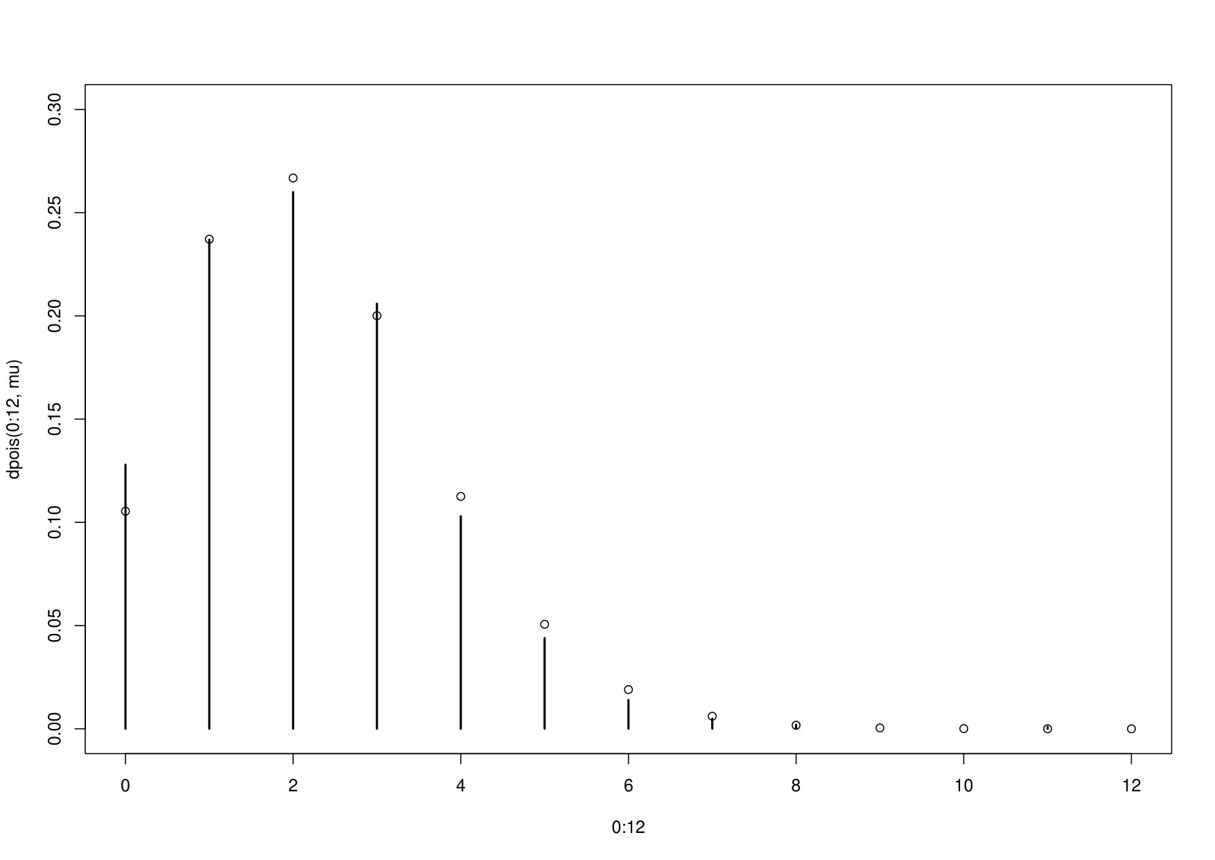 Figure 1
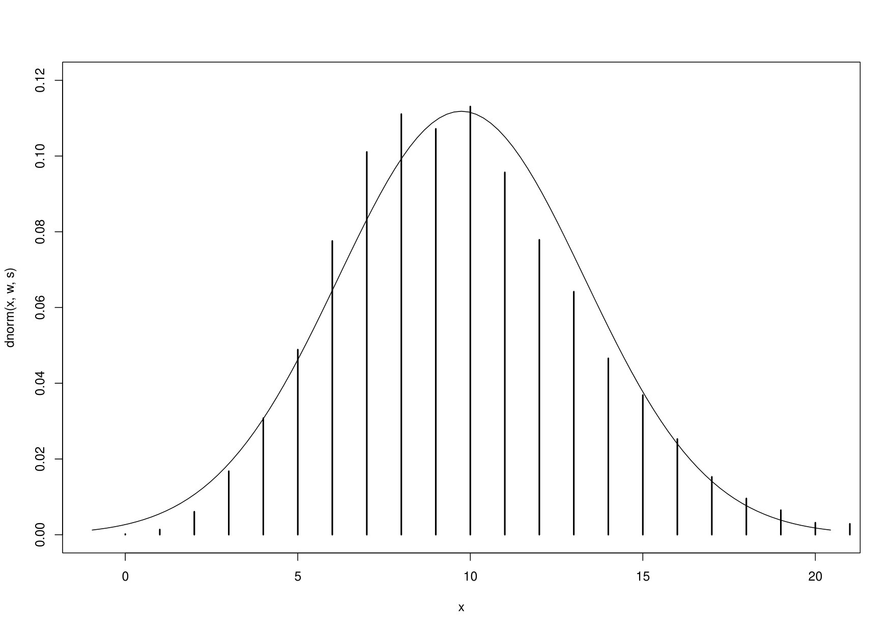 Figure 2
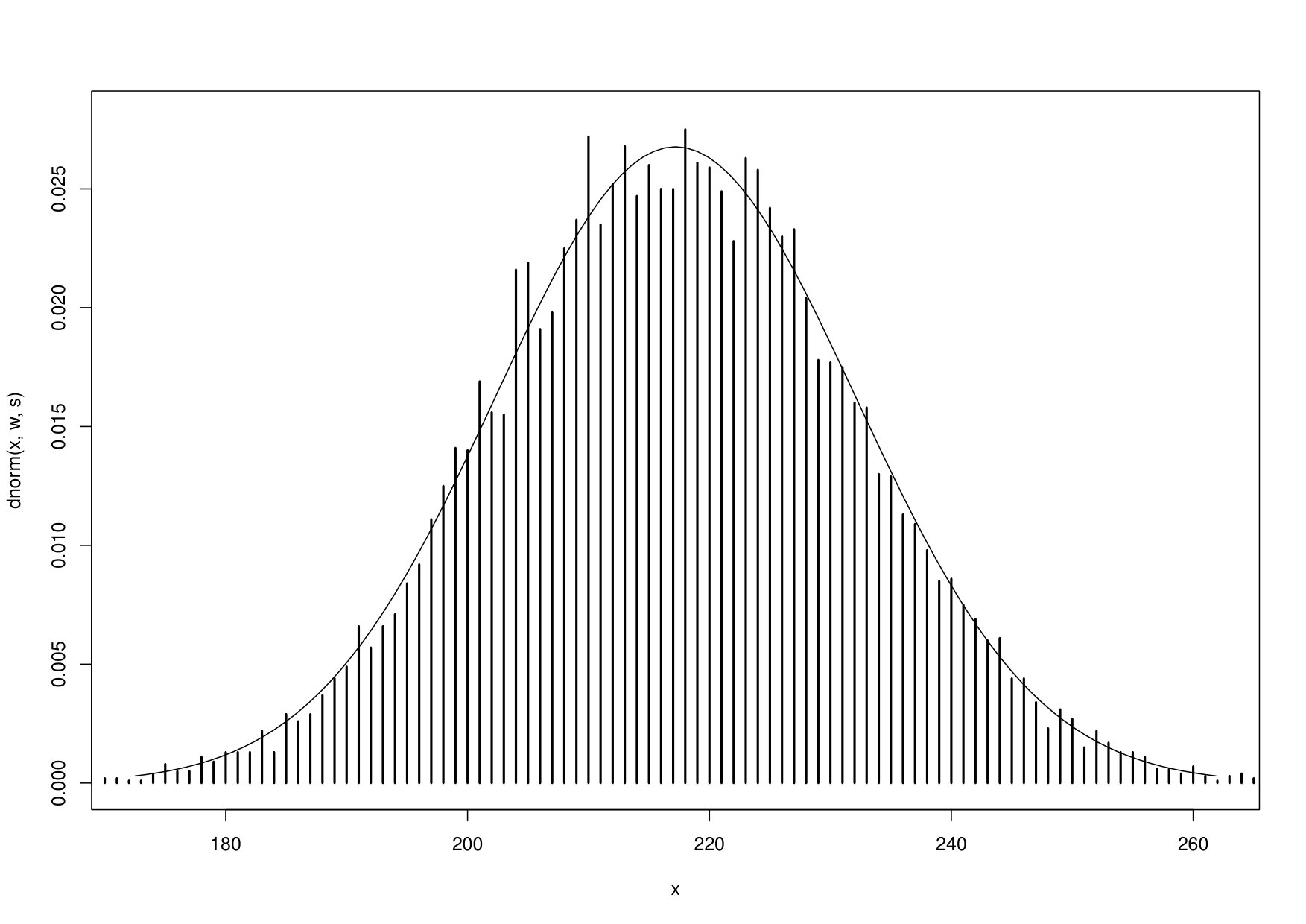 Figure 3
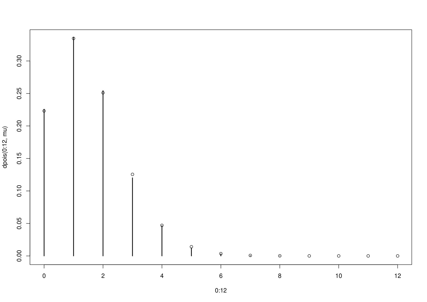 Figure 4
Peer Reviews
No public reviews on file for this paper yet. If you reviewed it on a platform where reviews are public (OpenReview, ICLR, NeurIPS, ICML), you can paste yours below so the community can read it here.
Videos
No videos yet. Explain this paper in a talk, walkthrough, or lecture? Add one.
Asymptotics of the overflow in urn models111This material is based upon work supported by and while serving at the National Science Foundation. Any opinion, findings, and conclusions or recommendations expressed in this material are
those of the authors and do not necessarily reflect the views of the National Science Foundation. 222Part of the research by the last two authors was carried out while they visited the Center for Mathematical Modeling at the University of Chile. They would like to thank the first author for arranging the visits and his hospitality, and the CMM for a generous support.
Raul Gouet Supported by grants PIA AFB-170001 and Fondecyt 1161319 Departamento de Ingenieria Matemática and CMM (UMI 2807, CNRS), Universidad de Chile
Paweł Hitczenko On leave from Drexel University Division of Mathematical Sciences, National Science Foundation
Jacek Wesołowski Supported by the grant 2016/21/B/ST1/00005 of National Science Centre, Poland Faculty of Mathematics and Information Science, Warsaw University of Technology
Abstract
Consider a number, finite or not, of urns each with fixed capacity and balls randomly distributed among them. An overflow is the number of balls that are assigned to urns that already contain balls. When , using analytic methods, Hwang and Janson gave conditions under which the overflow (which in this case is just the number of balls landing in non–empty urns) has an asymptotically Poisson distribution as the number of balls grows to infinity. Our aim here is to systematically study the asymptotics of the overflow in general situation, i. e. for arbitrary . In particular, we provide sufficient conditions for both Poissonian and normal asymptotics for general , thus extending Hwang–Janson’s work. Our approach relies on purely probabilistic methods.
Keywords and phrases: Urn model; occupancy problem; random allocations; weak limit theorems
MSC 2010 subject classifications: Primary 60F05, 60K30; secondary 60K35
1 Introduction
Urn models are one of the fundamental objects in classical probability theory and they have been studied for a long time in various degrees of generality. We refer the reader to classical sources [Johnson and Kotz (1977), Kolchin et al. (1978), Kotz and Balakrishnan (1997), Mahmoud (2009)] for a complete account of the theory and discussions of different models, and to e. g. [Gnedin et al. (2007), Hwang and Janson (2008), Bobecka et al. (2013)] for some of the more recent developments. Perhaps the most heavily studied characteristic is the number of occupied urns after balls have been thrown in. One reason for this is that it is often interpreted as a measure of diversity of a given population. Actually, more refined characteristics, e. g. the number of urns containing the prescribed number of balls, have been subsequently studied for various urn models. In diversity analysis, the number of urns with exactly balls, is called abundance count of order . In particular, the popular estimator of species richness, called Chao estimator, is based on and (with a more sophisticated version using also and ) - see e. g. [Chao and Chiu (2016)]. In [Hwang and Janson (2008)] the authors used analytical methods based on Poissonization and de–Poissonization to prove that the number of empty urns is asymptotically normal as long as its variance grows to infinity (this is clearly the minimal requirement). As a by–product of their method they established the Poissonian asymptotics of the number of balls that fall into non–empty urns when the variance is finite and under additional assumptions on the distribution among boxes. We mention in passing that the number of balls falling into non–empty urns is sometimes called the number of collisions. Under the uniformity assumption for the distribution of balls it has been used, for example, for testing random number generators (see [Knuth (1998), vol. 2, §3.3.2 I] for more details). We refer also to [Arratia et al. (2016)] and references therein for another illustration of how this concept is used, e.g. in cryptology.
Our main aim here is to extend the result of Hwang and Janson by considering the number of balls falling into urns containing at least balls (thus, their result corresponds to ). Relying on purely probabilistic methods we provide sufficient conditions for both Poissonian and normal asymptotics for the number of balls falling into such urns.
One way to formulate the problem is as follows. There is a collection (possibly infinite) of distinct containers in which balls are to be inserted. All containers have the same finite capacity. Each arriving ball is to be placed in one of the containers, randomly and independently of other balls. However, if the container selected for a given ball is already full, the ball lands in the overflow basket. We are interested in the number of balls in that basket when more and more balls appear. The notion of the overflow is not entirely new and has appeared, for example, in the context of collision resolution for hashing algorithms, see a discussion in section: “External searching” in [Knuth (1998), vol. 3, §6.4]. We also refer to subsequent work [Ramakrishna (1987), Monahan (1987)] for the computation of the probability that there is no overflow (under the uniformity assumption), and to [Dupuis et al. (2004)] which, in part, concerns the estimation of the probability of unusually large overflow. As far as we are aware, however, asymptotic behavior of the overflow has not been systematically investigated.
More precisely, we consider the following model: For any , let be iid rv’s with values in and let , be the common distribution among the boxes for each of the balls in the th experiment. Let also
[TABLE]
for any , and , where denotes the indicator of the events within brackets. That is is the number of balls among first balls for which the th box was selected.
Let be a given positive integer, which denotes the (same) capacity of every container. Then
[TABLE]
is 1 if the th ball lands in the overflow, and is 0 otherwise. Naturally, for . Consequently, the size of the overflow, denoted , can be written as
[TABLE]
We are interested in the asymptotic distribution of , as . We will show that there are regimes relating and under which the limiting distribution of (possibly standardized) is either Poisson or normal. These regimes will be defined through the limiting behavior of
[TABLE]
Actually, we impose assumptions on and .
1.1 Multinomial distribution and negative association
Note that, for distinct and any , has multinomial distribution . In particular, has the binomial distribution , that is,
[TABLE]
where . Also, let
[TABLE]
for , and , for . Then, for distinct and , has multinomial distribution . Moreover, vectors and are independent. Further, it is well known that multinomial random variables are negatively orthant dependent (NOD), that is, for
[TABLE]
As such they are also negatively associated (NA) - see [Joag-Dev and Proschan (1983)] for the definition and basic properties .
In particular, both sets and are NA and, by property , the combined set of and variables is also NA. In particular, by , for distinct , the subset , , , , is NA as well. Finally, noting that we conclude by that , , , are NA.
Consequently, the following extended versions of the NOD property (3) hold:
[TABLE]
and, taking in (4),
[TABLE]
1.2 Auxiliary random variables
We find it convenient to introduce sequences of random variables and such that, for any , the random variables are iid. This allows, in general, to simplify expressions because sums over can be represented as expectations and computations are compactly carried out by means of conditional expectations. For example,
[TABLE]
where here and everywhere below we write for .
Let be the -algebra generated by , for , and note that is -measurable, for any . Note also that, for any , is independent of . Then can be written as
[TABLE]
So, for ,
[TABLE]
Hence, , for , and .
Note that representation (7) implies
[TABLE]
Taking expectations of both extremes of (7) we get
[TABLE]
where . Furthermore, for , (8) yields
[TABLE]
and, because and are conditionally independent given , it follows that
[TABLE]
Consequently, for any ,
[TABLE]
2 Poissonian asymptotics
Let denote the Poisson distribution with parameter .
Theorem 2.1**.**
Let . If
[TABLE]
and
[TABLE]
then .
**Examples:
\bullet\** Consider the uniform case, that is, , for . Then by the above theorem we get
[TABLE]
Illustrative simulations are visualized in Figure 1.
\bullet\Consider the geometric case, , . Then
[TABLE]
Take (that is ). Thus, by (13), Moreover, .
Consequently, the above theorem yields with . Illustrative simulations are visualized in Figure 2.
The method of Poissonization and de–Poissonization was used in [Hwang and Janson (2008), Theorem 8.2] to prove Theorem 2.1, for . The proof we present here is entirely different and relies on the following martingale-type convergence result from [Beśka et al. (1982)].
Theorem 2.2**.**
Let be a double sequence of non-negative random variables, adapted to a row-wise increasing double sequence of -fields , and let . If
[TABLE]
[TABLE]
and, for any ,
[TABLE]
then .
In the proof of Theorem 2.1 we use the following consequences of (11) and (12).
Lemma 2.3**.**
Let be a positive integer. If (11) and (12) hold, then
[TABLE]
and
[TABLE]
Proof.
Since , (17) follows from (12). Also, (18) follows from (11) and (12) since
[TABLE]
∎
We also need the simple estimate shown below, for the tail of a binomial sum.
Lemma 2.4**.**
Let be positive integers, such that , and let . Then
[TABLE]
Proof.
The left-hand side of (19) is , where has distribution . Arguing by induction on , we have
[TABLE]
where the last inequality follows from . ∎
3 Proof of Theorem 2.1
Proof.
We show that for defined in (1), conditions (14), (15) with , and (16) are satisfied. First we note that (16) is trivially satisfied because, for , if and only if .
The rest of the proof is divided into three steps. In Step I we check that (14) is satisfied. Then we prove that (15) holds in quadratic mean, that is,
[TABLE]
To that end we show that and in Step II and Step III, respectively.
Step I: We prove (14) using (8). Clearly, , for , so
[TABLE]
Note also that, due to (9), (19) and (17),
[TABLE]
Consequently, Markov’s inequality implies and thus (14) follows.
Step II: To prove that we show that and are respectively bounded above and below by . From (9), (19) and (11)
[TABLE]
so .
Additionally, since by (9), and , we have
[TABLE]
Further, observe that
[TABLE]
Thus, by (11) and (18), the rhs of (20) converges to and so, .
Step III: We prove that , relying on the NOD property of , for distinct . In what follows we compute and bound some expectations that add up to . First note from (10) that
[TABLE]
For square-integrable random variables and a -algebra, let the conditional covariance be defined as
[TABLE]
Also, let (for simplicity) and . Then, by the iid assumption of , we have
[TABLE]
Furthermore,
[TABLE]
where the last equality follows from , for , because implies . So, from (21) and (22), we get
[TABLE]
Furthermore, by the NOD property (5),
[TABLE]
Hence, from (21) and (24), we have
[TABLE]
And, finally, from (23) and (25),
[TABLE]
which, after taking expectation, yields
[TABLE]
Also, by (19),
[TABLE]
Last, taking expectation above and adding over and , from (27) we obtain
[TABLE]
where convergence to 0 follows from (18). Finally, since , it follows that . ∎
4 Normal asymptotics for overflow
The following theorem gives conditions under which the overflow is asymptotically normal.
Theorem 4.1**.**
Assume that and that . Then
[TABLE]
Examples
Consider the uniform case, i.e. , . Then by the above theorem we get
[TABLE]
Note that with yields normal asymptotics.
Consider the geometric case, , , with and . Then (13) yields
[TABLE]
Moreover,
[TABLE]
Thus, asymptotic normality of follows from the above theorem. Illustrative simulations are visualized in Figures 3 and 4.
The proof of Theorem 4.1 is split in several steps given in four subsections below. In Subsection 4.1 we decompose in the sum of martingale differences , with suitably defined (uniformly bounded) ’s. In Subsection 4.2 we show that is of order . In Subsection 4.3 we show that is of order . The final part of the proof, which gathers all previous steps, is given in Subsection 4.4.
4.1 Martingale differences decomposition
Lemma 4.2**.**
The centered size of the overflow can be represented as , where the are martingale differences defined by
[TABLE]
Proof.
Clearly, . Further, noting that is the trivial -algebra,
[TABLE]
∎
Lemma 4.3**.**
The martingales differences of (28) are uniformly bounded and can be represented as
[TABLE]
Proof.
Let and note that . For simplicity let and . Then
[TABLE]
Hence, noting that , we have
[TABLE]
Consequently, from (7), we can write
[TABLE]
and, similarly,
[TABLE]
Also, note that
[TABLE]
Therefore, for ,
[TABLE]
Thus
[TABLE]
Observe that, for , \mathbb{E}\,\Big{(}\tfrac{I_{\{X_{n,j}=X_{n}\}}}{p_{X_{n}}}|X_{n},\mathcal{F}_{n,j-1}\Big{)}=1. Then
[TABLE]
Note that , is equal to on the event . That is, using the original notation,
[TABLE]
on the event and so,
[TABLE]
Finally, since
[TABLE]
we conclude that
[TABLE]
For the boundedness of note that
[TABLE]
∎
4.2 Asymptotic variance
Lemma 4.4**.**
Assume that and that . Then
[TABLE]
Proof.
Let , and
[TABLE]
Then
[TABLE]
and so
[TABLE]
Also, recalling that are iid,
[TABLE]
where the second equality above follows from the conditional independence of and , given .
In what follows we compute by considering the cases and . We get
[TABLE]
where the second equality above follows from conditioning inside both expectations above, with respect to . Finally, integrating out in the first expectation, we obtain
[TABLE]
and, consequently,
[TABLE]
For the upper bound of the variance note that and thus (34) implies
[TABLE]
Also,
[TABLE]
and so,
[TABLE]
Now, recalling that has distribution , for , and using (19), the rhs of (35) is bounded by . Last, taking expectations, we obtain and, consequently,
[TABLE]
Now, to bound the variance of from below, we first find an upper bound for the last term (with minus sign) in display (34). To that end note that , defined in (32), can be written as
[TABLE]
where is , independent of , so
[TABLE]
and
[TABLE]
Furthermore, for , let be , independent of and independent of . Then
[TABLE]
can be written as
[TABLE]
and so,
[TABLE]
Then, since, conditionally on , is and because of the NOD property, we have
[TABLE]
where the second equality follows from the NOD property and the third from (37). Finally, taking expectations and using the independence of and , we get
[TABLE]
Replacing the rightmost expectation in display (34) by the bound above we have
[TABLE]
Note that
[TABLE]
Hence, since ,
[TABLE]
Finally note that , as defined in (32), can be written in the form
[TABLE]
where and . Therefore,
[TABLE]
Since it follows that the double sum above is non-negative and so,
[TABLE]
Consequently,
[TABLE]
and finally, since ,
[TABLE]
∎
4.3 Variance of the sum of conditional variances
Lemma 4.5**.**
Under the hypotheses of Lemma 4.4
[TABLE]
Proof.
We first rewrite (33) as
[TABLE]
where
[TABLE]
Consequently, letting , and noting that , we have
[TABLE]
Then
[TABLE]
and the analogous formula holds for . In what follows we express the variances and covariances of in terms of . For simplicity, let , then
[TABLE]
where and are such that are iid for any . We only check the first formula; the others are obtained similarly.
[TABLE]
[TABLE]
and the formula for follows. We now compute bounds for the covariances in (42). Since and are bounded above by reasoning as in the paragraph preceding (36), we have,
[TABLE]
and
[TABLE]
Next, we handle , which requires somewhat more effort than the previous covariances because the crude bounds do not yield the right order in . Since ,
[TABLE]
because each of the remaining three covariances is bounded by an expression of the form . To bound the covariance between and we write
[TABLE]
and note that the first expectation in (46) is bounded by
[TABLE]
where is a positive constant. For the second expectation in (46) we have the following expression, written in terms of (conditionally independent) binomial random variables .
[TABLE]
Conditionally on , are independent, with distributed and distributed . Further, are independent of , conditionally on .
Note that (48) can be rewritten as
[TABLE]
where and . Note also that, for , and are NOD; see (5). Thus, conditioning on the values of the binomials, using the NOD property; then integrating over the ’s and using independence of and , we have the following upper bound for (49)
[TABLE]
which, after ignoring the indicator and noting that the conditional probabilities (on and ) are independent random variables, can be finally bounded by
[TABLE]
Therefore, from (45), (46), (47) and (50), we have
[TABLE]
It remains to bound the covariances . To that end we consider first, the expected value of the product.
[TABLE]
where is the event that are all distinct. Then,
[TABLE]
Note that, as in (48), the first term on the rhs of (52) can be written as follows
[TABLE]
Conditionally on , are independent, where is , is , is and is . Also, are independent of , conditionally on . Now, using the NOD property (4) and the independence of , , the expression in (54) is bounded above by
[TABLE]
Therefore, from (52), (53) and (55),
[TABLE]
We complete the proof of (38) by collecting the partial results above to obtain bounds for and , using formula (41). From (43) and (44) we have
[TABLE]
[TABLE]
Last, from (56)
[TABLE]
The conclusion follows from (40), (41) and the bounds for the sums of variances and covariances above. ∎
4.4 Final touch - the martingale CLT
We show the asymptotic normality by applying the martingale central limit theorem (see e. g. [Helland (1982), Theorem 2.5] to the martingale differences . Since ’s are uniformly bounded the conditional Lindeberg condition ([Helland (1982), condition (2.5)]) follows from the fact that the variance of the sum grows to infinity as . The remaining condition to be checked ([Helland (1982), condition (2.7)]) is that
[TABLE]
as or, equivalently, that
[TABLE]
But this follows immediately from Lemma 4.4, Lemma 4.5 and Chebyshev’s inequality.
5 Asymptotics for number of full containers with and without overflow
Let denote the number of full containers and denote number of full containers without overflow. The main idea is to represent and in terms of the size of the overflow .
Recall that is the total number of balls in the sample for which the th box was selected. Thus
[TABLE]
We note that
[TABLE]
That is,
[TABLE]
and
[TABLE]
Note that in the case we have and thus , which is a number of non-empty boxes, is
[TABLE]
and , which is number of singleton boxes, is
[TABLE]
These representations of and in terms of , and allow to read Poissonian asymptotics of these two sequences from Theorem 2.1. For the forthcoming statement was proved in [Kolchin et al. (1978), Theorem III.3.1].
Theorem 5.1**.**
Assume that .
If and then
[TABLE] 2. 2.
If and then
[TABLE]
Proof.
The case : Due to representations (57) and (58) to prove both results it suffices to show that for any fixed . But following the argument from the beginning of Step II of the proof of Theorem 2.1 we see that
[TABLE]
where the convergence to zero in the last step follows from Lemma 2.3.
The case : The first part follows from Theorem 2.1 since (59) implies . The second follows also from Theorem 2.1 since (60) gives
[TABLE]
and, similarly as in the case , we have . ∎
Note that under assumptions of Th. 5.1
- •
in case 1: ,
- •
in case 2:
Representations (57) and (58) are also useful for getting Gaussian asymptotics of and from Theorem 4.1 in the case .
Theorem 5.2**.**
Assume that and .
If then
[TABLE] 2. 2.
If then
[TABLE]
Proof.
By representation (57) we can write
[TABLE]
Since it follows that . Therefore by Lemma 4.4 we have
[TABLE]
and thus also
[TABLE]
Consequently, . Thus the first result is a consequence of Theorem 4.1 since, in view of the representation (57),
[TABLE]
For the second case, by representation (58) we can write
[TABLE]
Similarly as in the previous case we conclude that for . Therefore, by the same argument as above it follows that each of the summands at the right hand side above except the first one converges to 0 as . Consequently, , . Thus the second result is a consequence of Theorem 4.1 since, in view of (58),
[TABLE]
∎
The reference list from the paper itself. Each links out to its DOI / PubMed record.
- 1[Arratia et al. (2016)] Arratia, R., Garibaldi, S., Kilian, J. Asymptotic distribution for the birthday problem with multiple coincidences, via an embedding of the collision process. Random Structures & Algorithms 48 (2016), 480–502.
- 2[Beśka et al. (1982)] Beśka, M., Kłopotowski, A., Słomiński, L. Limit theorems for random sums of dependent d 𝑑 d -dimensional random vectors. Z. Wahrschein. verw. Geb. 61 (1982), 43–57.
- 3[Bobecka et al. (2013)] Bobecka, K., Hitczenko, P., López-Blázquez, F., Rempała, G., Wesołowski, J. Asymptotic normality through factorial cumulants and partition identities. Combin. Probab. Comput. 22(2) (2013), 213–240.
- 4[Chao and Chiu (2016)] Chao, A., Chiu, C.-H. Species richness: estimation and comparison. Wiley Stats Ref: Statistics Reference Online, 1–26.
- 5[Dupuis et al. (2004)] Dupuis, P., Nuzman, C., Whiting, P. Large deviation asymptotics for occupancy problems. Ann. Probab. 32 (2004), 2765–2818.
- 6[Gnedin et al. (2007)] Gnedin, A., Hansen, B., Pitman, J. , Notes on the occupancy problem with infinitely many boxes: general asymptotics and power laws. Probab. Surv. 4 (2007), 146–171.
- 7[Helland (1982)] Helland, I. S. , Central limit theorems for martingales with discrete or continuous time. Scand. J. Statist. 9 (1982), 79–94.
- 8[Hwang and Janson (2008)] Hwang, H.K., Janson, S. Local limit theorems for finite and infinite urn models. Ann. Probab. 36(3) (2008), 992–1022.