Amplitude analysis of the $B_{(s)} \to K^{*0} \overline{K}^{*0}$ decays and measurement of the branching fraction of the $B \to K^{*0} \overline{K}^{*0}$ decay
LHCb Collaboration: R. Aaij, C. Abell\'an Beteta, B. Adeva, M., Adinolfi, C.A. Aidala, Z. Ajaltouni, S. Akar, P. Albicocco, J. Albrecht, F., Alessio, M. Alexander, A. Alfonso Albero, G. Alkhazov, P. Alvarez Cartelle,, A.A. Alves Jr, S. Amato, Y. Amhis, L. An, L. Anderlini

TL;DR
This paper performs an amplitude analysis of B meson decays to K*0 pairs, measuring polarization fractions and branching ratios, providing insights into decay dynamics and CP violation in these processes.
Contribution
It introduces a detailed amplitude analysis of B0 and Bs decays to K*0 pairs, measuring polarization and branching fractions with improved precision.
Findings
Longitudinal polarization fraction for B0 decay is 0.724
Branching fraction for B0 decay is (8.0 ± 0.9)×10^{-7}
Different polarization behaviors observed between B0 and Bs decays
Abstract
The and decays are studied using proton-proton collision data corresponding to an integrated luminosity of 3fb. An untagged and time-integrated amplitude analysis of decays in two-body invariant mass regions of 150 MeV around the mass is performed. A stronger longitudinal polarisation fraction in the decay, , is observed as compared to in the decay. The ratio of branching fractions of the two decays is measured and used to determine .
Click any figure to enlarge with its caption.
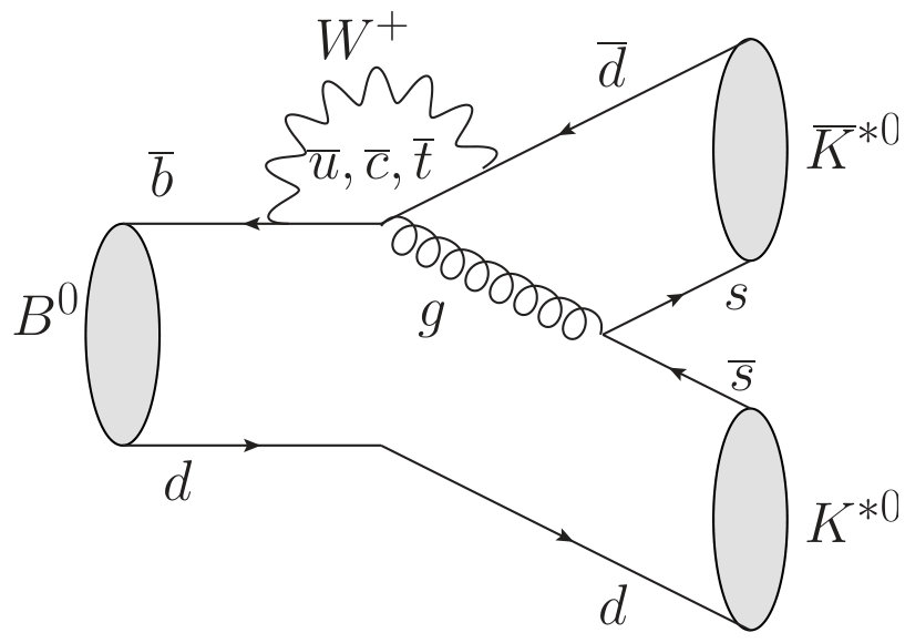 Figure 1
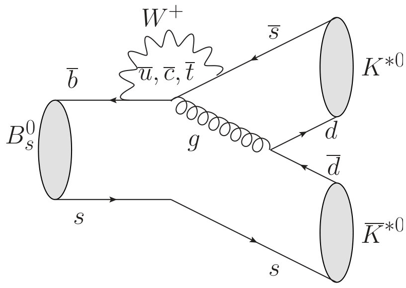 Figure 1
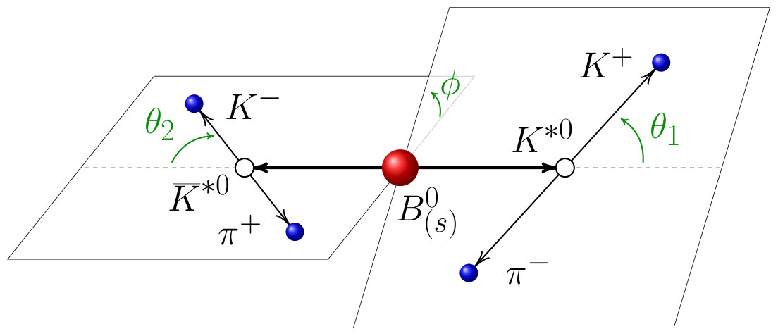 Figure 2
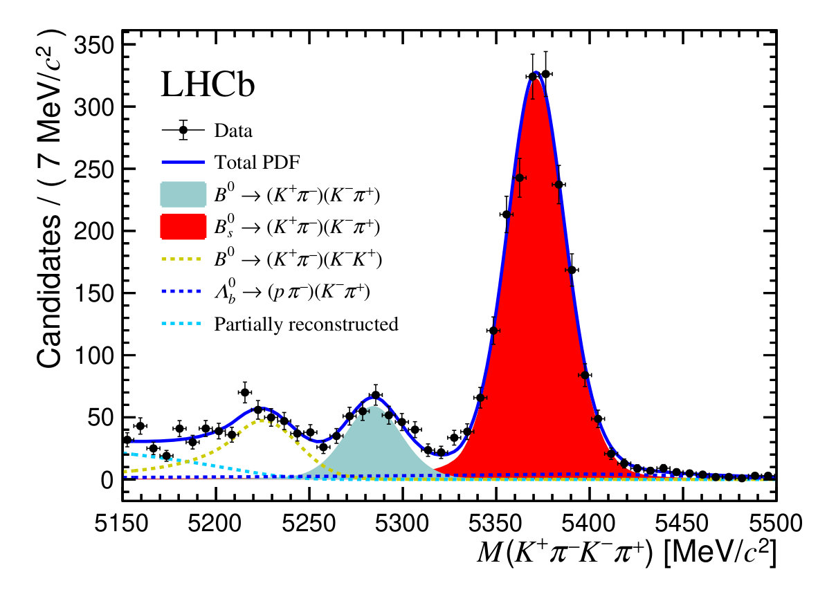 Figure 3
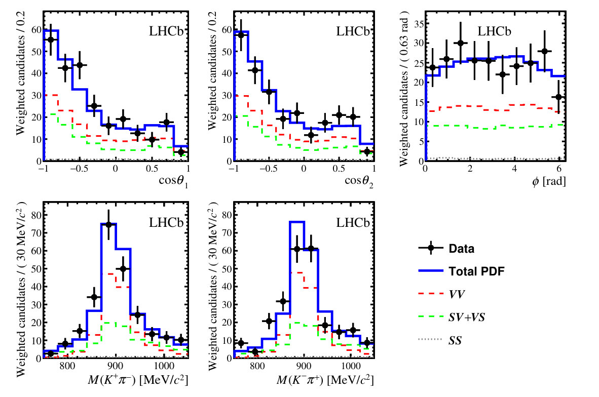 Figure 4
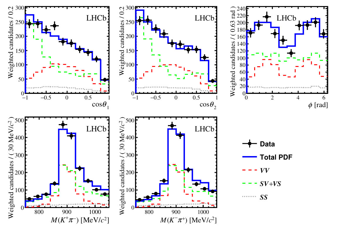 Figure 5
| 1 | |||
| 2 | |||
| 3 | |||
| 4 | |||
| 5 | |||
| 6 |
| Yield | 2011 sample | 2012 sample |
|---|---|---|
| Misidentified | ||
| Partially reconstructed background | ||
| Combinatorial background |
| Parameter | ||
|---|---|---|
| S–wave fraction |
| [MeV/],, | ||||
|---|---|---|---|---|
| [MeV] | ||||
| [/GeV] | ||||
| [/GeV] | ||||
| Decay mode | |||||||||
|---|---|---|---|---|---|---|---|---|---|
| Parameter | |||||||||
| Bias data-simulation | 0.001 | 0.00 | 0.006 | 0.004 | 0.01 | 0.00 | 0.01 | ||
| Fit method | 0.007 | 0.01 | 0.011 | 0.001 | 0.00 | 0.00 | 0.02 | ||
| Kinematic acceptance | 0.005 | 0.01 | 0.006 | 0.002 | 0.03 | 0.01 | 0.04 | ||
| Resolution | 0.007 | 0.00 | 0.005 | 0.002 | 0.00 | 0.00 | 0.02 | ||
| P–wave mass model | 0.001 | 0.00 | 0.004 | 0.002 | 0.00 | 0.00 | 0.02 | ||
| S–wave mass model | 0.007 | 0.01 | 0.016 | 0.002 | 0.03 | 0.03 | 0.02 | ||
| Differences data-simulation | 0.004 | 0.00 | 0.002 | 0.001 | 0.01 | 0.01 | 0.01 | ||
| Background subtraction | 0.002 | 0.01 | 0.006 | 0.002 | 0.01 | 0.01 | 0.09 | ||
| Peaking backgrounds | 0.009 | 0.02 | 0.009 | 0.003 | 0.04 | 0.01 | 0.08 | ||
| \cdashline1-10 Total systematic unc. | 0.016 | 0.03 | 0.024 | 0.006 | 0.06 | 0.04 | 0.13 | ||
| Decay mode | |||||
|---|---|---|---|---|---|
| Observable | S–wave fraction | ||||
| Bias data-simulation | 0.001 | 0.002 | 0.007 | ||
| Fit method | 0.000 | 0.000 | 0.006 | ||
| Kinematic acceptance | 0.003 | 0.003 | 0.006 | ||
| Resolution | 0.001 | 0.001 | 0.006 | ||
| P–wave mass model | 0.000 | 0.001 | 0.005 | ||
| S–wave mass model | 0.000 | 0.002 | 0.008 | ||
| Differences data-simulation | 0.001 | 0.001 | 0.002 | ||
| Background subtraction | 0.005 | 0.001 | 0.002 | ||
| Peaking backgrounds | 0.010 | 0.002 | 0.009 | ||
| \cdashline1-10 Total systematic unc. | 0.012 | 0.004 | 0.017 | ||
| Decay mode | ||||||||
|---|---|---|---|---|---|---|---|---|
| Year | 2011 | 2012 | 2011 | 2012 | ||||
| Trigger | TOS | noTOS | TOS | noTOS | TOS | noTOS | TOS | noTOS |
| Bias data-simulation | 0.01 | 0.03 | 0.02 | 0.01 | 0.04 | 0.03 | 0.02 | 0.02 |
| Fit method | 0.00 | 0.00 | 0.00 | 0.00 | 0.00 | 0.00 | 0.00 | 0.00 |
| Kinematic acceptance | 0.03 | 0.04 | 0.02 | 0.02 | 0.06 | 0.06 | 0.06 | 0.06 |
| Resolution | 0.02 | 0.02 | 0.02 | 0.02 | 0.00 | 0.00 | 0.00 | 0.00 |
| P–wave mass model | 0.02 | 0.02 | 0.02 | 0.02 | 0.05 | 0.04 | 0.05 | 0.04 |
| S–wave mass model | 0.03 | 0.03 | 0.03 | 0.03 | 0.17 | 0.17 | 0.16 | 0.17 |
| Differences data-simulation | 0.01 | 0.01 | 0.01 | 0.01 | 0.01 | 0.01 | 0.01 | 0.01 |
| Background subtraction | 0.03 | 0.03 | 0.03 | 0.03 | 0.02 | 0.01 | 0.02 | 0.01 |
| Peaking backgrounds | 0.03 | 0.04 | 0.03 | 0.04 | 0.01 | 0.01 | 0.01 | 0.01 |
| Time acceptance | 0.08 | 0.07 | 0.08 | 0.07 | ||||
| \cdashline1-9 Total systematic unc. | 0.06 | 0.08 | 0.06 | 0.07 | 0.19 | 0.19 | 0.17 | 0.18 |
| Parameter | 2011 TOS MagUp | 2011 TOS MagDown | 2011 noTOS MagUp | 2011 noTOS MagDown |
|---|---|---|---|---|
Peer Reviews
No public reviews on file for this paper yet. If you reviewed it on a platform where reviews are public (OpenReview, ICLR, NeurIPS, ICML), you can paste yours below so the community can read it here.
Videos
No videos yet. Explain this paper in a talk, walkthrough, or lecture? Add one.
EUROPEAN ORGANIZATION FOR NUCLEAR RESEARCH (CERN)
CERN-EP-2019-063
LHCb-PAPER-2019-004
July 16, 2019
Amplitude analysis of the decays and measurement of the branching fraction of the decay
The LHCb collaboration†††Authors are listed at the end of this letter.
The and decays are studied using proton-proton collision data corresponding to an integrated luminosity of 3. An untagged and time-integrated amplitude analysis of decays in two-body invariant mass regions of 150 around the mass is performed. A stronger longitudinal polarisation fraction in the decay, , is observed as compared to in the decay. The ratio of branching fractions of the two decays is measured and used to determine {\mathcal{B}}(\mbox{{{B}^{0}}!\rightarrow{{K}^{*0}}{{\kern 1.79993pt\overline{\kern-1.79993ptK}}{}^{*0}}})=(8.0\pm 0.9\,({\rm stat})\pm 0.4\,({\rm syst}))\times 10^{-7}.
Published in JHEP 07 (2019) 032
© 2024 CERN for the benefit of the LHCb collaboration. CC-BY-4.0 licence.
1 Introduction
The decay is a Flavour-Changing Neutral Current (FCNC) process.111Throughout the text charge conjugation is implied, indicates either a or a pair, indicates either a or a meson and refers to the resonance, unless otherwise stated. In the Standard Model (SM) this type of processes is forbidden at tree level and occurs at first order through loop penguin diagrams. Hence, FCNC processes are considered to be excellent probes for physics beyond the SM, since contributions mediated by heavy particles, contemplated in these theories, may produce effects measurable with the current sensitivity.
Evidence of the decay has been found by the BaBar collaboration [1] with a measured yield of decays. An untagged time-integrated analysis was presented finding a branching fraction of and a longitudinal polarisation fraction of . In untagged time-integrated analyses the distributions for and decays are assumed to be identical and summed, so that they can be fitted with a single amplitude. However, if -violation effects are present, the distribution is given by the incoherent sum of the two contributions. The Belle collaboration also searched for this decay [2] and a branching fraction of was measured, disregarding S–wave contributions. There is a standard-deviations difference between the branching fraction measured by the two experiments. The predictions of factorised QCD (QCDF) are and [3]. Perturbative QCD predicts [4].222This reference considers two scenarios for its predictions, both giving compatible results. Only the first scenario considered therein is quoted here. These theoretical predictions agree with the experimental results within the large uncertainties. The measurement of agrees with the naïve hypothesis, based on the quark helicity conservation and the V$$-$$A nature of the weak interaction, that charmless decays into pairs of vector mesons () should be strongly longitudinally polarised. See, for example, the Polarization in B Decays review in Ref. [5].
The decay was first observed by the LHCb experiment with early LHC data [4]. A later untagged time-integrated study, with data corresponding to of integrated luminosity, measured and [6]. More recently, a complete -sensitive time-dependent analysis of decays in the mass range from 750 to has been published by LHCb [7], with data corresponding to of integrated luminosity. A determination of was performed as well as the first measurements of the mixing-induced -violating phase and of the direct asymmetry parameter . These LHCb analyses of decays lead to three conclusions: firstly, within their uncertainties, the measured observables are compatible with the absence of violation; secondly, a low polarisation fraction is found; finally, a large S–wave contribution, as much as , is measured in the window around the mass. The low longitudinal polarisation fraction shows a tension with the prediction of QCDF ( [3]) and disfavours the hypothesis of strongly longitudinally polarised decays. Theoretical studies try to explain the small longitudinal polarisation with mechanisms such as contributions from annihilation processes [8, 3]. It is intriguing that the two channels and , which are related by U-spin symmetry, implying the exchange of and quarks as displayed in Fig. 1, show such different polarisations. A comprehensive theory review on polarisation of charmless neutral -meson decays can be found in Ref. [9].
Some authors consider the decay as a golden channel for a precision test of the CKM phase [10]. High-precision analyses of this channel, dominated by the gluonic-penguin diagram, will require to account for subleading amplitudes [11, 9]. The study of the decay allows to control higher-order SM contributions to the channel employing U-spin symmetry [10, 12]. In Refs. [12, 13] more precise QCDF predictions, involving the relation between longitudinal branching fractions of the two channels, are made.
In this work, an untagged and time-integrated amplitude analysis of the and decays in the two-body invariant mass regions of 150 around the mass is presented, as well as the determination of the decay branching fraction. The analysis uses data recorded in 2011 and 2012 at centre-of-mass energies of and , respectively, corresponding to an integrated luminosity of .
This paper is organised as follows. In Sect. 2 the formalism of the decay amplitudes is presented. In Sect. 3 a brief description of the LHCb detector, online selection algorithms and simulation software is given. The selection of and candidates is presented in Sect. 4. Sect. 5 describes the maximum-likelihood fit to the four-body invariant-mass spectra and its results. The amplitude analysis and its results are discussed in Sect. 6. The estimation of systematic uncertainties is described in Sect. 7, and the determination of the decay branching fraction relative to the mode in Sect. 8. Finally, the results are summarised and conclusions are drawn in Sect. 9.
2 Amplitude analysis formalism
The and modes are weak decays of a pseudoescalar particle into two vector mesons (). The -meson decays are followed by subsequent and decays. The study of the angular distribution employs the helicity angles shown in Fig. 2: , defined as the angle between the direction of the meson and the direction opposite to the -meson momentum in the rest frame of the () resonance, and , the angle between the decay planes of the two vector mesons in the -meson rest frame. From angular momentum conservation, three relative polarisations of the final state are possible for final states that correspond to longitudinal ([math] or ), or transverse to the direction of motion and parallel () or perpendicular () to each other. For the two-body invariant mass of the and pairs, noted as and , a range of 150$$\text{\,Me\kern-1.00006ptV\!/}c^{2} around the known mass [5] is considered. Therefore, pairs may not only originate from the spin-1 meson, but also from other spin states. This justifies that, besides the helicity angles, a phenomenological description of the two-body invariant mass spectra, employing the isobar model, is adopted in the analytic model. In the isobar approach, the decay amplitude is modelled as a linear superposition of quasi-two-body amplitudes [14, *Morgan:1968zza, *Herndon:1973yn].
For the S–wave (), the resonance, the possible (or ) and a non-resonant component, , need to be accounted for. This is done using the LASS parameterisation [17], which is an effective-range elastic scattering amplitude, interfering with the meson,
[TABLE]
where
[TABLE]
represents the width. In Eq. (1) and Eq. (2) is the centre-of-mass decay momentum, and , and are the mass, width and centre-of-mass decay momentum at the pole, respectively. The effective-range elastic scattering amplitude component depends on
[TABLE]
where is the scattering length and the effective range.
For the P–wave (), only the resonance is considered. Other P–wave resonances, such as or , with pole masses much above the fit region, are neglected. Resonances with higher spin, for instance the D–wave meson, are negligible in the considered two-body mass range [7] and are also disregarded. The amplitude is parameterised with a spin-1 relativistic Breit–Wigner amplitude,
[TABLE]
The mass-dependent width is given by
[TABLE]
where and are the mass and width, is the interaction radius parameterising the centrifugal barrier penetration factor, and corresponds to the centre-of-mass decay momentum at the resonance pole. The values of the mass propagator parameters are summarised in Table 1.
The differential decay rate for mesons333Charge conjugation is not implied in the rest of this section. For the charge-conjugated mode, , the decay rate is obtained applying the transformation in Eq. (5) where the corresponding eigenvalues, , are given in Table 2. at production is given by [19, 6],
[TABLE]
where is the four-body phase space factor. The index runs over the first column of Table 2 where the different decay amplitudes, , and the angular-mass functions, , are listed. The angular dependence of these functions is obtained from spherical harmonics as explained in Ref. [19]. For -studies, the -odd, , and -even, , eigenstates of the S–wave polarisation amplitudes are preferred to the vector-scalar () and scalar-vector () helicity amplitudes, to which they are related by
[TABLE]
The remaining amplitudes, except for , correspond to -even eigenstates. The contributions can be quantified by the terms , defined as
[TABLE]
which are normalised according to
[TABLE]
This condition ensures that .
The polarisation fractions of the amplitudes are defined as
[TABLE]
where , and are the longitudinal, parallel and transverse amplitudes of the P–wave. Therefore, is the fraction of longitudinally polarised decays. The polarisation fractions are preferred to the amplitude moduli since they are independent of the considered mass range. The P–wave amplitudes moduli can always be recovered as
[TABLE]
The phase of all propagators is set to be zero at the mass. In addition, a global phase can be factorised without affecting the decay rate setting . The last two requirements establish the definition of the amplitude phases (, , , and ) as the phase relative to that of the longitudinal P–wave amplitude at the mass.
Since mesons oscillate, the decay rate evolves with time. The time-dependent amplitudes are obtained replacing and in Eq. (5) being
[TABLE]
with
[TABLE]
where and are the widths of the light and heavy mass eigenstates of the system and and are their masses. The coefficients p and q are the mixing terms that relate the flavour and mass eigenstates,
[TABLE]
Masses and widths are often considered in their averages and differences, , , and , in particular in their relation with the mixing phase,
[TABLE]
In this analysis, no attempt is made to identify the flavour of the initial meson and time-integrated spectra are considered. Consequently, the selected candidates correspond to untagged and time-integrated decay rates and there is no sensitivity to direct and mixing-induced violation. Moreover, since the origin of phases is set in a -even eigenstate (), for the -odd eigenstates, the untagged time-integrated decay is only sensitive to the phase difference . The present experimental knowledge is compatible with small violation in mixing [20] and with the absence of direct violation in the system [7].
The dependence of the decay rate in an untagged and time-integrated analysis of a meson can be expressed as
[TABLE]
where the amplitudes account for the the average of and decays and is a normalisation constant. For the meson, a further simplification of the decay rate is considered, since [20] the light and heavy mass eigenstate widths can be assumed to be equal,
[TABLE]
and this factor can be extracted as part of the normalisation constant in Eq. (8). For the meson the central values {\Gamma_{\mathrm{H}}}=0.618$$\text{\,ps}^{-1} and {\Gamma_{\mathrm{L}}}=0.708$$\text{\,ps}^{-1} [20] are considered.
3 Detector and simulation
The LHCb detector [21, 22] is a single-arm forward spectrometer covering the pseudorapidity range , designed for the study of particles containing or quarks. The detector includes a high-precision tracking system consisting of a silicon-strip vertex detector surrounding the interaction region, a large-area silicon-strip detector located upstream of a dipole magnet with a bending power of about , and three stations of silicon-strip detectors and straw drift tubes placed downstream of the magnet. The tracking system provides a measurement of the momentum, , of charged particles with a relative uncertainty that varies from 0.5% at low momentum to 1.0% at 200. The minimum distance of a track to a primary vertex (PV), the impact parameter (IP), is measured with a resolution of , where is the component of the momentum transverse to the beam, in . Different types of charged hadrons are distinguished using information from two ring-imaging Cherenkov detectors. Photons, electrons and hadrons are identified by a calorimeter system consisting of scintillating-pad and preshower detectors, an electromagnetic and a hadronic calorimeter. Muons are identified by a system composed of alternating layers of iron and multiwire proportional chambers.
The magnetic field deflects oppositely charged particles in opposite directions and this can lead to detection asymmetries. Periodically reversing the magnetic field polarity throughout the data-taking almost cancels the effect. The configuration with the magnetic field pointing upwards (downwards), MagUp (MagDown), bends positively (negatively) charged particles in the horizontal plane towards the centre of the LHC ring.
The online event selection is performed by a trigger [23], which consists of a hardware stage, based on information from the calorimeter and muon systems, followed by a software stage, which applies a full event reconstruction. In the offline selection, trigger signatures are associated with reconstructed particles. Since the trigger system uses the of the charged particles, the phase-space and time acceptance is different for events where signal tracks were involved in the trigger decision (called trigger-on-signal or TOS throughout) and those where the trigger decision was made using information from the rest of the event only (noTOS).
Simulated samples of the and decays with longitudinal polarisation fractions of 0.81 and 0.64, respectively, are primarily employed in these analyses, particularly for the acceptance description as explained in Sect. 6. Simulated samples of the main peaking background contributions, , and , are also considered. In the simulation, collisions are generated using Pythia [24] with a specific LHCb configuration [25]. Decays of hadronic particles are described by EvtGen [26], in which final-state radiation is generated using Photos [27]. The interaction of the generated particles with the detector, and its response, are implemented using the Geant4 toolkit [28, 29] as described in Ref. [30].
4 Signal selection
Both data and simulation are filtered with a preliminary selection. Events containing four good quality tracks with p_{\mathrm{T}}>500$$\text{\,Me\kern-1.00006ptV\!/}c are retained. In events that contain more than one PV, the candidate constructed with these four tracks is associated with the PV that has the smallest , where is defined as the difference in the vertex-fit of the PV reconstructed with and without the track or tracks in question. Each of the four tracks must fulfil with respect to the PV and originate from a common vertex of good quality (, where ndf is the number of degrees of freedom of the vertex). To identify kaons and pions, a selection in the difference of the log-likelihoods of the kaon and pion hypothesis () is applied. This selection is complemented with fiducial constraints that optimise the particle identification determination: the pion and kaon candidates are required to have 3<p<100$$\text{\,Ge\kern-1.00006ptV\!/}c and and be inconsistent with muon hypothesis. The final state opposite charge pairs are combined into and candidates with a mass within 150$$\text{\,Me\kern-1.00006ptV\!/}c^{2} of the mass. The and candidates must have p_{\mathrm{T}}>900$$\text{\,Me\kern-1.00006ptV\!/}c and vertex . The intermediate resonances must combine into candidates within 500$$\text{\,Me\kern-1.00006ptV\!/}c^{2} of the mass, with a distance of closest approach between their trajectories of less than mm. To guarantee that the candidate originates in the interaction point, the cosine of the angle between the momentum and the direction of flight from the PV to the decay vertex is required to be larger than 0.99 and the with respect to the PV has to be smaller than 25.
A multivariate selection based on a Boosted Decision Tree with Gradient Boost [31, *Roe] (BDTG) is employed. It relies on the aforementioned variables and on the candidate flight distance with respect to the PV and its . Simulated decays with tracks matched to the generator particles and filtered with the preliminary selection are used as signal sample, whereas the four-body invariant-mass sideband , composed of purely combinatorial combinations, is used as background sample for the BDTG training. The number of events in the signal training sample of the BDTG is determined using the ratio between the and the yields from Ref. [6] and the yield obtained with a four-body mass fit to the data sample after the preliminary selection. The number of events in the background training sample of the BDTG is estimated by extrapolating the background yield in the sideband into the \pm 30$$\text{\,Me\kern-1.00006ptV\!/}c^{2} window around the mass. The requirement on the BDTG output is chosen to maximise the figure of merit , where and are the expected output signal and background yields, respectively. Different BDTGs are implemented for 2011 and 2012 data.
A comprehensive search for peaking backgrounds, mainly involving intermediate charm particles, is performed. Decays of mesons sharing the same final state with the signal,444The branching fractions in this section are taken from Ref. [5]. such as () and () decays, are strongly suppressed by the requirement in the mass. Resonances in three-body combinations ( ) and ( ) are also explored. In the case of the former, the three-body invariant mass in the data sample is above all known charm resonances. For the latter, no evidence of candidates originated in and decays () or in decays () is found. Three-body combinations with a pion misidentified as a kaon are reconstructed, mainly searching for decays (), but also for (), and () decays. All of them are suppressed to a negligible level by the applied selection. A search of three-body combinations with a proton misidentified as a kaon is performed, finding no relevant contribution from decays involving a baryon. Decays into five final-state particles are also investigated. Contributions of the decay can be neglected due to the small misidentification probability and the four-body mass distribution whereas the decay is negligible due to the requirement on the mass.
5 Four-body mass spectrum
The signal and background yields are determined by means of a simultaneous extended maximum-likelihood fit to the invariant-mass spectra of the four final-state particles in the 2011 and 2012 data samples. The signal decays are parameterised with double-sided Hypatia distributions [33] with the same parameters except for their means that are shifted by the difference between the and masses, [5]. Misidentified (including decays), and decays are also considered in the fit. Both the and contributions are described with the sum of a Crystal Ball [34] function and a Gaussian distribution which shares mean with the Crystal Ball core. The parameters of these distributions are obtained from simulation, apart from the mean and resolution values which are free to vary in the fit. Whereas the distribution mean values are constrained to be the same in the 2011 and 2012 data, the resolution is allowed to have different values for the two samples. The small contributions from and decays have a broad distribution in the four-body mass and are the object of specific treatment. The contribution from decays has an expected yield of () in the 2011 (2012) sample. It is estimated from the detection and selection efficiency measured with simulation, the collected luminosities, the cross section for production, the hadronisation fractions of and mesons and the known branching fraction of the mode. Simulated events containing this decay mode are added with negative weights to the final data sample to subtract its contribution. The contribution of decays in the 2011 (2012) sample is determined to be () from a fit to the four-body mass spectrum of the selected data. In this study the four-body invariant mass is recomputed assigning the proton mass to the kaon with the largest value. In these fits the component is described with a Gaussian distribution and the dominant background is described with a Crystal Ball function. The parameters of both lineshapes are obtained from simulation. The remaining contributions, mainly and partially reconstructed events, are parameterised with a decreasing exponential with a free decay constant. The decay angular distribution is currently unknown and its contribution can not be subtracted with negatively weighted simulated events. Its subtraction is commented further below.
Finally, contributions from partially reconstructed -hadron decays and combinatorial background are also considered. The former is composed of - and -meson decays containing neutral particles that are not reconstructed. Because of the missing particle, the measured four-body invariant mass of these candidates lies in the lower sideband of the spectrum. All contributions to this background are jointly parameterised with an ARGUS function [35] convolved with a Gaussian resolution function, with the same width as the signal. The endpoint of the distribution is also fixed to the mass minus the mass. The combinatorial background is composed of charged tracks that are not originating from the signal decay chain. It is modelled with a linear distribution, with a free slope parameter, separate for 2011 and 2012 data samples.
The results of the fit to the four-body mass spectrum are shown in Fig. 3 and the yields are reported in Table 3. In total, about three hundred signal candidates are found, a factor seven larger than previous analyses [1, 2]. To perform a background-subtracted amplitude analysis, the sPlot technique [36, 37] is applied to isolate either the or the decays. The contribution from , for which the yield is fixed, is treated using extended weights according to Appendix B.2 of Ref. [36]. The sPlot method suppresses the background contributions using their relative abundance in the four-body invariant mass spectrum and, therefore, no assumption is required for their phase-space distribution.
6 Amplitude analysis
Each of the background-subtracted samples of and decays is the object of a separate amplitude analysis based on the model described in Sect. 2. As a first step, the effect of a non-uniform efficiency, depending on the helicity angles and the two-body invariant masses, is examined. For this purpose, four categories are defined according to the hardware trigger decisions (TOS or noTOS) and data-taking period (2011 and 2012). The efficiency is accounted for through the complex integrals [38]
[TABLE]
where is the total phase-space dependent efficiency, is the sample category and are defined in Eq. (6). The integrals of Eq. (9) are determined using simulated signal samples of each of the four categories, selected with the same criteria applied to data. A single set of integrals is used for both the and the amplitude analyses. A probability density function (PDF) for each category is built
[TABLE]
where and are given in Table 2.
Candidates from all categories are processed in a simultaneous unbinned maximum-likelihood fit, separately for each signal decay mode, using the PDFs in Eq. (10). To avoid nonphysical values of the parameters during the minimisation, some of them are redefined as
[TABLE]
where , and are used in the fit, together with , ,, , and . The former three variables are free to vary within the range , ensuring that the sum of all the squared amplitudes is never greater than . The fit results are corrected for a small reducible bias, originated in discrepancies between data and simulation, as explained in Sect. 7. The final results are shown in Table 4.
Figs. 4 and 5 show the one-dimensional projections of the amplitude fit to the and signal samples in which the background is statistically subtracted by means of the sPlot technique. Three contributions are shown: , produced by pairs originating in a decay; , accounting for amplitudes in which only one of the pairs originates in a decay; and , where none of the two pairs originate in a decay.
The fraction of decays, or purity at production, of the signal, , is estimated from the amplitude analysis and found to be
[TABLE]
The significance of this magnitude, computed as its value over the sum in quadrature of the statistical and systematic uncertainty, is found to be 10.8 standard deviations. This significance corresponds to the presence of decays in the data sample. The S–wave fraction of the decay is equal to . For the mode the S–wave fraction is found to be .
7 Systematic uncertainties of the amplitude analysis
Several sources of systematic uncertainty that affect the results of the amplitude analysis are considered and discussed in the following.
Fit method. Biases induced by the fitting method are evaluated with a large ensemble of pseudoexperiments. For each signal decay, samples with the same yield of signal observed in data (see Table 3) are generated according to the PDF of Eq. (8) with inputs set to the results summarised in Table 4. The use of the weights defined in Eq. (9) to account the detector acceptance would require a full simulation and, instead, a parametric efficiency is considered. For each observable, the mean deviation of the result from the input value is assigned as a systematic uncertainty.
Description of the kinematic acceptance. The uncertainty on the signal efficiency relies on the coefficients of Eq. (9) that are estimated with simulation. To evaluate its impact on the amplitude analysis results, the fit to data is repeated several times with alternative coefficients varied according to their covariance matrix. The standard deviation of the distribution of the fit results for each observable is assigned as a systematic uncertainty.
Resolution. The fit performed assumes a perfect resolution on the phase-space variables. The impact of the detector resolution on these variables is estimated with sets of pseudoexperiments adding per-event random deviations according to the resolution estimated from simulation. For each observable, the mean deviation of the result from the measured value is assigned as a systematic uncertainty.
P–wave** mass model.** The amplitude analysis is repeated with alternative values of the parameters that define the P–wave mass propagator, detailed in Table 1, randomly sampled from their known values [5]. The standard deviation of the distribution of the amplitude fit results for each observable is assigned as a systematic uncertainty.
S–wave** mass model.** In addition to the default S–wave propagator, described in Sect. 2, two alternative models are used: the LASS lineshape with the parameters of Table 5, obtained with decays within the analysis of Ref. [39], and the propagator proposed in Ref. [40]. The amplitude fit is performed with these two alternatives and, for each observable, the largest deviation from the baseline result is assigned as a systematic uncertainty.
Differences between data and simulation. An iterative method [41], is used to weight the simulated events and improve the description of the track multiplicity and -meson momentum distributions. The procedure is repeated multiple times and, for each observable, the mean bias of the amplitude fit result is corrected for in the results of Table 4 while its standard deviation is assigned as a systematic uncertainty.
Background subtraction. The data set used in the amplitude analysis is background subtracted using the sPlot method [36, 37] that relies in the lineshapes of the four-body mass fit discussed in Sect. 5. The uncertainty related to the determination of the signal weights is evaluated repeating the amplitude analysis fits with weights obtained fitting the four-body invariant-mass with two alternative models. In the first case, the model describing the signal is defined by the sum of two Crystal Ball functions [34] with a common, free, peak value and the resolution parameter fixed from simulation. In the second case, the model describing the combinatorial background is assumed to be an exponential function. The amplitude fit is performed with the sPlot-weights obtained with the two alternatives and, for each observable, the largest deviation from the baseline result is assigned as a systematic uncertainty. This procedure is also used when addressing the systematic uncertainties in the measured yields of the different subsamples, as discussed in Sect. 8.
Peaking backgrounds. The uncertainty related to the fluctuations in the yields of the and background contributions are estimated repeating the amplitude-analysis fit with the yield values varied by their uncertainties reported in Sect. 5. For each observable, the largest deviation from the default result is assigned as a systematic uncertainty. This procedure is also used when addressing the systematic uncertainties of the four-body invariant mass yields in Sect. 8.
Time acceptance. The amplitude analysis does not account for possible decay-time dependency of the efficiency, however, the trigger and the offline selections may have an impact on it. This effect only affects -meson decays and is accounted for by estimating effective shifts: {\Gamma_{\mathrm{H}}}=0.618\rightarrow 0.598$$\text{\,ps}^{-1} and {\Gamma_{\mathrm{L}}}=0.708\rightarrow 0.732$$\text{\,ps}^{-1}, which are obtained with simulation. For each observable, the variation of the result of the fit after introducing these values in the amplitude analysis is considered as a systematic uncertainty.
The resulting systematic uncertainties and the corrected biases, originated in the differences between data and simulation, are detailed in Table 6 for the parameters of the amplitude-analysis fit. The corresponding values for the derived observables are summarised in Table 7. The total systematic uncertainty is computed as the sum in quadrature of the different contributions.
8 Determination of the ratio of branching fractions
In this analysis, the branching fraction is measured relative to that of decays. Since both decays are selected in the same data sample and share a common final state most systematic effects cancel. However, some efficiency corrections, eg. those originated from the difference in phase-space distributions of events of the two modes, need to be accounted for. The amplitude fit provides the relevant information to tackle the differences between the two decays.
This branching-fraction ratio is obtained as
[TABLE]
where, for each channel, is the detection efficiency, is a polarisation-dependent correction of the efficiency, originated in differences between the measured polarisation and that assumed in simulation, is the measured number of candidates and represents the signal purity at detection. In this way represents the yield. Finally, and are the hadronisation fractions of a -quark into a and meson, respectively.
The purity at detection and the factor ratios, , are obtained for each decay mode as
[TABLE]
where the coefficients are defined in Eq. (9), are the amplitudes used to generate signal samples, and the values are given in Table 2. Also in this case, for the decay, the approximation is adopted.
The detection efficiency is determined from simulation for each channel separately for the different categories discussed in Sect. 6: year of data taking, trigger type and, in addition, the LHCb magnet polarity. An exception is applied to the particle-identification selection whose efficiency is determined from large control samples of , decays. Differences in kinematics and detector occupancy between the control samples and the signal data are accounted for in this particle-identification efficiency study [42, 43].
The different sources of systematic uncertainty in the branching fraction determination are discussed below.
Systematic uncertainties in the factor . The uncertainties on the parameters of the amplitude analysis fit described in Sect. 7 affect the determination of the factors defined in Eq. (12) as summarised in Table 8.
Systematic uncertainties in the signal yields. As discussed in Sect. 7 uncertainties on the signal yields arise from the model used to fit the four-body invariant mass. The uncertainties from the different proposed alternative signal and background lineshapes are summed in quadrature to compute the final systematic uncertainty.
Systematic uncertainty in the efficiencies. A dedicated data method is employed to estimate the uncertainty in the signal efficiency originated in the PID selection.
The inputs employed for measuring the relative branching fraction are summarised in Table 9. The factor is different for the two decay modes because of two main reasons: firstly, the discrepancy between the polarisation assumed in simulation and its measurement is larger for the than for the decay. Secondly, the different S–wave fraction of the decays. Also, the efficiency ratio of the two modes deviating from one is explained upon the different polarisation of the simulation samples. The LHCb detector is less efficient for values of () close to unity because of slow pions emitted in () decays and these are more frequent the larger is the longitudinal polarisation.
The final result of the branching-fraction ratio is obtained as the weighted mean of the per-category result obtained with Eq. (11) for the eight categories of Table 9, and found to be
[TABLE]
Considering that
[TABLE]
from Ref. [5], the absolute branching fraction for the mode is found to be
[TABLE]
It is worth noticing that, since the branching fraction was determined with the decay as a reference [6], the uncertainty on , which appears in the ratio of Eq. (13), does not contribute to the absolute branching fraction measurement.
9 Summary and final considerations
The first study of decays is performed with a data set recorded by the LHCb detector, corresponding to an integrated luminosity of 3.0 at centre-of-mass energies of 7 and 8 TeV. The mode is observed with standard deviations. An untagged and time-integrated amplitude analysis is performed, taking into account the three helicity angles and the and invariant masses in a 150 window around the and masses. Six contributions are included in the fit: three correspond to the P–wave, and three to the S–wave, along with their interferences. A large longitudinal polarisation of the decay, , is measured. The S–wave fraction is found to be .
A parallel study of the mode within of the mass is performed, superseding a previous LHCb analysis [6]. A small longitudinal polarisation, and a large S–wave contribution of are measured for the decay, confirming the previous LHCb results of the time-dependent analysis of the same data [7].
The ratio of branching fractions
[TABLE]
is determined. With this ratio the branching fraction is found to be
[TABLE]
This value is smaller than the measurement from the BaBar collaboration [1], due to the S–wave contribution. The measurement is compatible with the QCDF prediction of Ref. [3]: .
Using the -meson averages [20] for and the mixing phase, defined in Eq. (7), , the ratio
[TABLE]
is found to be
[TABLE]
This result is inconsistent with the prediction of [13]. Within models such as QCDF or the soft-collinear effective theory, based on the heavy-quark limit the predictions, longitudinal observables, such as the one in Eq. (14), have reduced theoretical uncertainties as compared to parallel and perpendicular ones. The heavy-quark limit also implies the polarisation hierarchy . The measured value for and the result of the decay put in question this hierarchy. The picture is even more intriguing since, contrary to its U-spin partner, the decay is confirmed to be strongly polarised.
Acknowledgements
We express our gratitude to our colleagues in the CERN accelerator departments for the excellent performance of the LHC. We thank the technical and administrative staff at the LHCb institutes. We acknowledge support from CERN and from the national agencies: CAPES, CNPq, FAPERJ and FINEP (Brazil); MOST and NSFC (China); CNRS/IN2P3 (France); BMBF, DFG and MPG (Germany); INFN (Italy); NWO (Netherlands); MNiSW and NCN (Poland); MEN/IFA (Romania); MSHE (Russia); MinECo (Spain); SNSF and SER (Switzerland); NASU (Ukraine); STFC (United Kingdom); DOE NP and NSF (USA). We acknowledge the computing resources that are provided by CERN, IN2P3 (France), KIT and DESY (Germany), INFN (Italy), SURF (Netherlands), PIC (Spain), GridPP (United Kingdom), RRCKI and Yandex LLC (Russia), CSCS (Switzerland), IFIN-HH (Romania), CBPF (Brazil), PL-GRID (Poland) and OSC (USA). We are indebted to the communities behind the multiple open-source software packages on which we depend. Individual groups or members have received support from AvH Foundation (Germany); EPLANET, Marie Skłodowska-Curie Actions and ERC (European Union); ANR, Labex P2IO and OCEVU, and Région Auvergne-Rhône-Alpes (France); Key Research Program of Frontier Sciences of CAS, CAS PIFI, and the Thousand Talents Program (China); RFBR, RSF and Yandex LLC (Russia); GVA, XuntaGal and GENCAT (Spain); the Royal Society and the Leverhulme Trust (United Kingdom).
The reference list from the paper itself. Each links out to its DOI / PubMed record.
- 1[1] Ba Bar collaboration, B. Aubert et al. , Observation of B 0 → K ∗ 0 K ¯ ∗ 0 {{B}^{0}}\!\rightarrow{{K}^{*0}}{{\kern 1.79993 pt\overline{\kern-1.79993 pt K}}{}^{*0}} and search for B 0 → K ∗ 0 K ∗ 0 → superscript 𝐵 0 superscript 𝐾 absent 0 superscript 𝐾 absent 0 B^{0}\rightarrow{K}^{*0}{K}^{*0} , Phys. Rev. Lett. 100 (2008) 081801 , ar Xiv:0708.2248 · doi ↗
- 2[2] Belle collaboration, C.-C. Chiang et al. , Search for B 0 → K ∗ 0 K ¯ ∗ 0 {{B}^{0}}\!\rightarrow{{K}^{*0}}{{\kern 1.79993 pt\overline{\kern-1.79993 pt K}}{}^{*0}} , B 0 → K ∗ 0 K ∗ 0 → superscript 𝐵 0 superscript 𝐾 absent 0 superscript 𝐾 absent 0 B^{0}\rightarrow K^{*0}K^{*0} and B 0 → K + π − K ∓ π ± → superscript 𝐵 0 superscript 𝐾 superscript 𝜋 superscript 𝐾 minus-or-plus superscript 𝜋 plus-or-minus B^{0}\rightarrow K^{+}\pi^{-}K^{\mp}\pi^{\pm} decays , Phys. Rev. D 81 (20 · doi ↗
- 3[3] M. Beneke, J. Rohrer, and D. S. Yang, Branching fractions, polarisation and asymmetries of B → V V → 𝐵 𝑉 𝑉 B\rightarrow VV decays , Nucl. Phys. B 774 (2007) 64 , ar Xiv:hep-ph/0612290 · doi ↗
- 4[4] LH Cb collaboration, R. Aaij et al. , First observation of the decay B s 0 → K ∗ 0 K ¯ ∗ 0 {{B}^{0}_{s}}\rightarrow{{K}^{*0}}{{\kern 1.79993 pt\overline{\kern-1.79993 pt K}}{}^{*0}} , Phys. Lett. B 709 (2012) 50 , ar Xiv:1111.4183 · doi ↗
- 5[5] Particle Data Group, M. Tanabashi et al. , Review of particle physics , Phys. Rev. D 98 (2018) 030001 · doi ↗
- 6[6] LH Cb collaboration, R. Aaij et al. , Measurement of C P 𝐶 𝑃 C\!P asymmetries and polarisation fractions in B s 0 → K ∗ 0 K ¯ ∗ 0 {{B}^{0}_{s}}\rightarrow{{K}^{*0}}{{\kern 1.79993 pt\overline{\kern-1.79993 pt K}}{}^{*0}} decays , JHEP 07 (2015) 166 , ar Xiv:1503.05362 · doi ↗
- 7[7] LH Cb collaboration, R. Aaij et al. , First measurement of the C P 𝐶 𝑃 C\!P -violating phase ϕ s d d ¯ superscript subscript italic-ϕ 𝑠 𝑑 ¯ 𝑑 \phi_{s}^{d{\overline{d}}} in B s 0 → ( K + π − ) ( K − π + ) → subscript superscript 𝐵 0 𝑠 superscript 𝐾 superscript 𝜋 superscript 𝐾 superscript 𝜋 {{B}^{0}_{s}}\rightarrow(K^{+}\pi^{-})(K^{-}\pi^{+}) decays , JHEP 03 (2018) 140 , ar Xiv:1712.08683 · doi ↗
- 8[8] A. L. Kagan, Polarization in B → V V → 𝐵 𝑉 𝑉 B\rightarrow VV decays , Phys. Lett. B 601 (2004) 151 , ar Xiv:hep-ph/0405134 · doi ↗