TL;DR
This paper presents MoGlow, a probabilistic, controllable motion synthesis model based on normalising flows, capable of generating complex, realistic motion sequences efficiently for interactive applications.
Contribution
It introduces a novel autoregressive, causal normalising flows model for motion synthesis that handles long-term dependencies without task-specific assumptions.
Findings
Outperforms baseline models in motion quality
Generates realistic motion close to real motion capture
Efficient training via exact maximum likelihood
Abstract
Data-driven modelling and synthesis of motion is an active research area with applications that include animation, games, and social robotics. This paper introduces a new class of probabilistic, generative, and controllable motion-data models based on normalising flows. Models of this kind can describe highly complex distributions, yet can be trained efficiently using exact maximum likelihood, unlike GANs or VAEs. Our proposed model is autoregressive and uses LSTMs to enable arbitrarily long time-dependencies. Importantly, is is also causal, meaning that each pose in the output sequence is generated without access to poses or control inputs from future time steps; this absence of algorithmic latency is important for interactive applications with real-time motion control. The approach can in principle be applied to any type of motion since it does not make restrictive, task-specific…
Click any figure to enlarge with its caption.
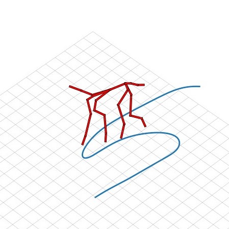 Figure 1
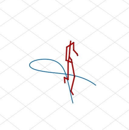 Figure 2
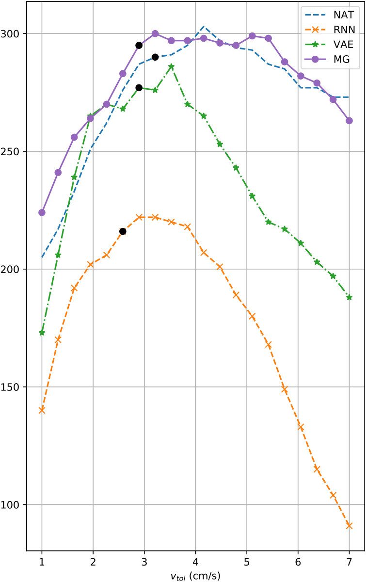 Figure 3
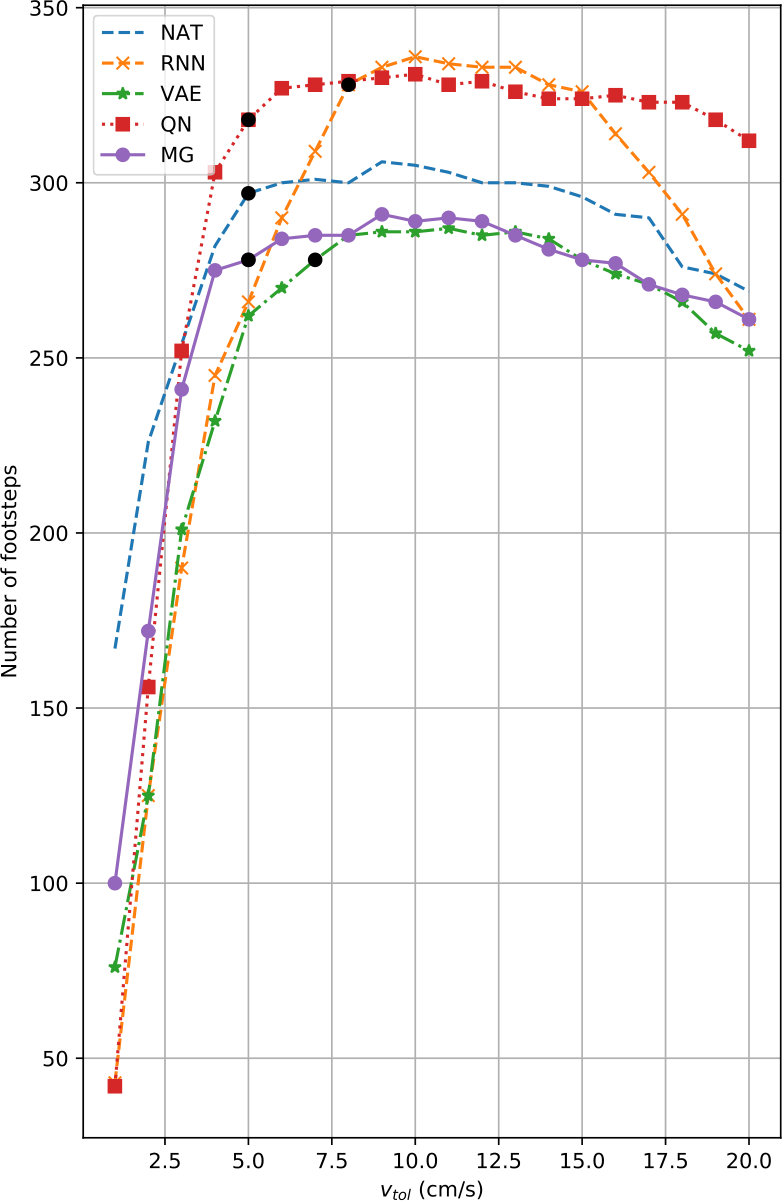 Figure 4
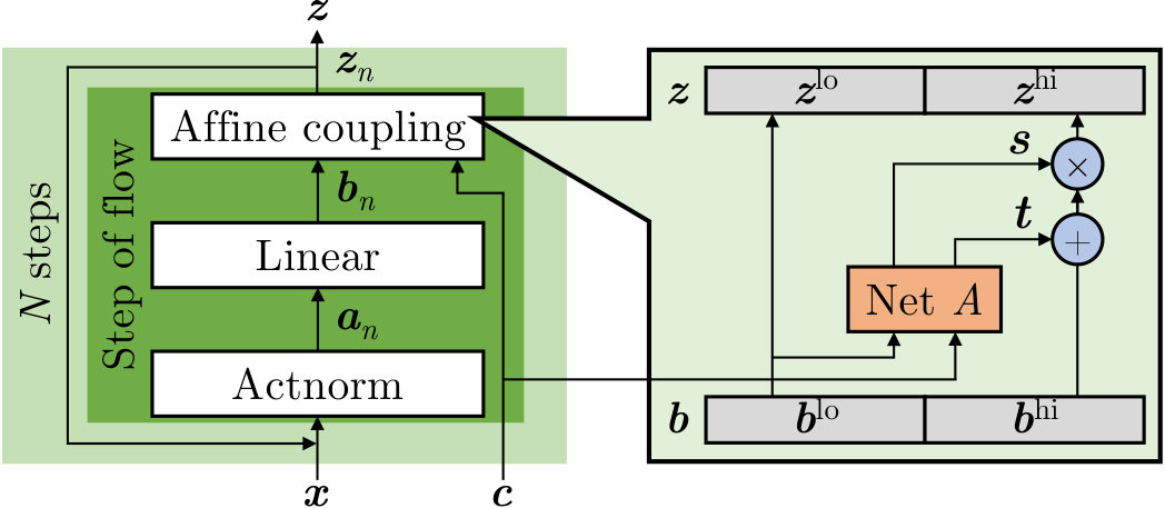 Figure 5
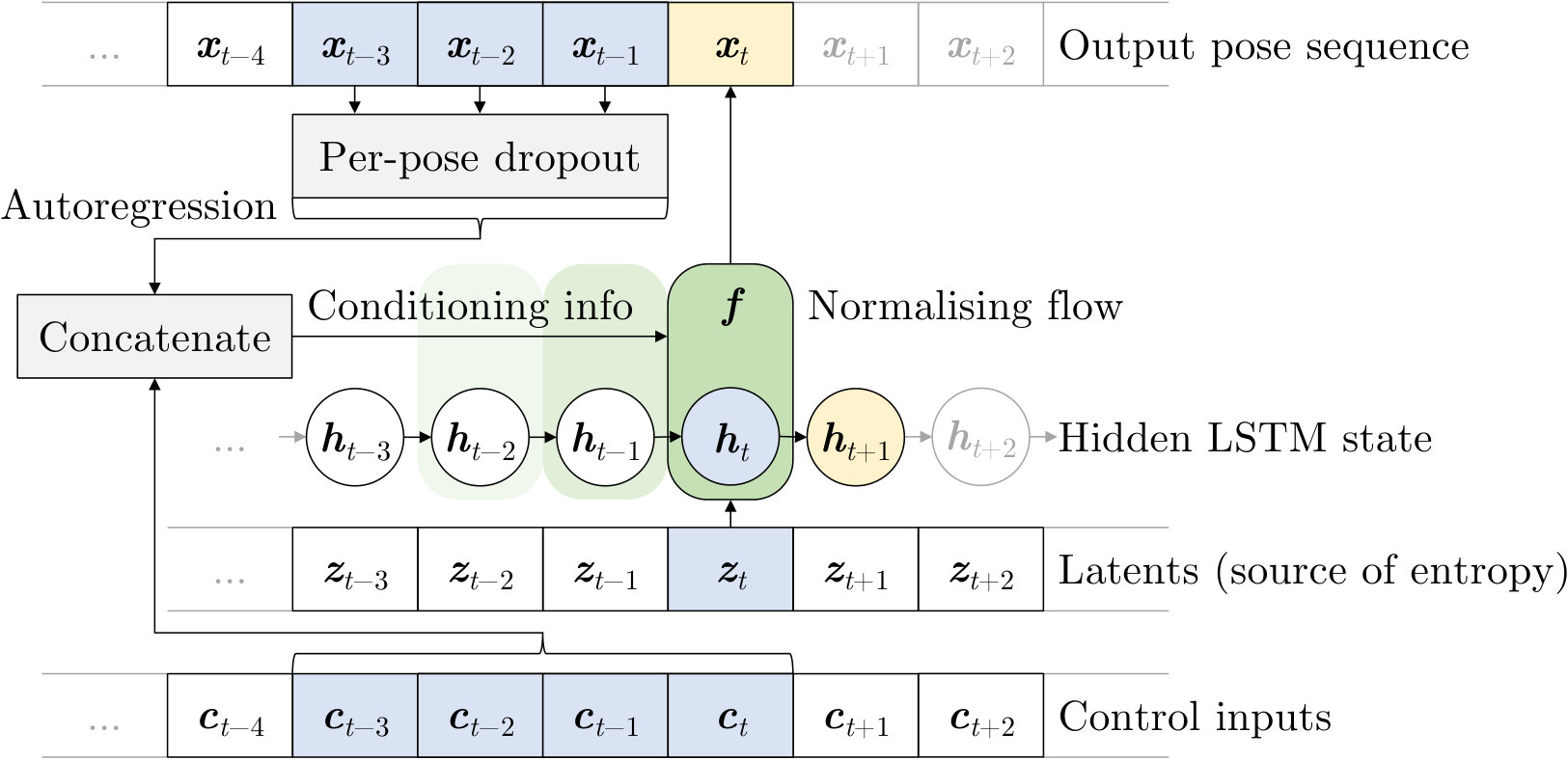 Figure 6
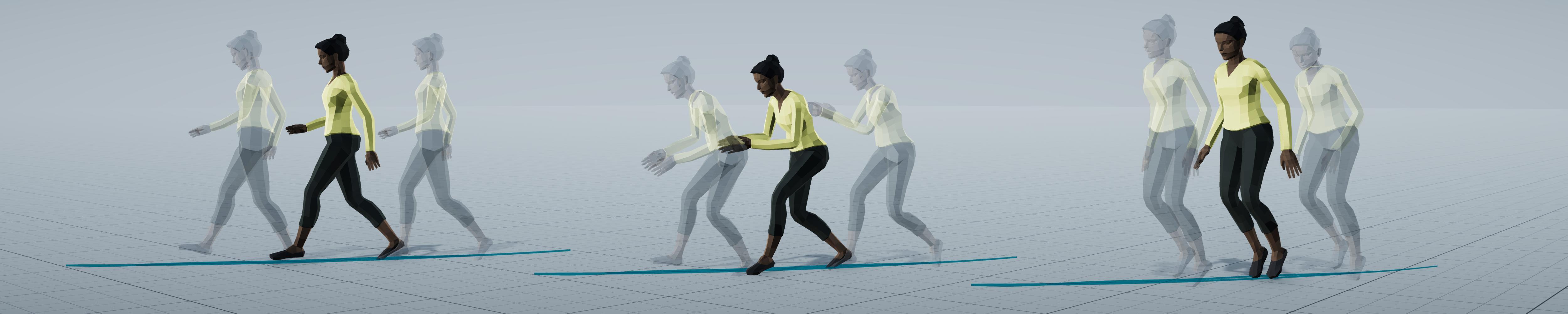 Figure 7
| Proba- | Task- | Algo. | Context | Hidden | Pose | Num. params. | Training… | |||||||
| Configuration | ID | bilistic? | agnostic? | latency | frames | state | dropout | Man | Dog | Loss func. | Epochs | Time | GPUs | |
| Baselines | Plain LSTM | RNN | ✗ | ✓ | None | - | LSTM | - | 01M | 01M | MSE | 40 | 0.7hh | 8 |
| Greenwood et al. (2017a) | VAE | Partially | ✓ | Full seq. | - | BLSTM | - | 04M | 04M | MSE+KLD | 40 | 6.1hh | 8 | |
| Pavllo et al. (2018) | QN | ✗ | ✗ | 1 sec. | - | GRU | - | 10M | - | Angl./pos.+reg. | 2k/4k | 10hh | 2 | |
| Zhang et al. (2018) | MA | ✗ | ✗ | 1 sec. | 12 | - | - | - | 05M | MSE | 150 | 30d h | 1 | |
| MoGlow | MG | ✓ | ✓ | None | 10 | LSTM | 95% | 74M | 80M | Log-likelihood | 291h | 26hh | 1 | |
| Ablats. | No pose dropout | MG-D | " | " | " | 10 | " | 0% | 74M | - | " | " | 26hh | " |
| No pose context | MG-A | " | " | " | 10 | " | 100% | 74M | - | " | " | 26hh | " | |
| Minimal history | MG-H | " | " | " | 1 | " | 95% | 54M | - | " | " | 23hh | " | |
| Human | Quadruped | |||
| ID | Held-out | Synthetic | Held-out | Synthetic |
| NAT | 4.270.11** | - | 4.25 0.06** | - |
| RNN | 3.100.15** | 1.90.2** | 2.81 0.10** | 1.14 0.04** |
| VAE | 3.950.13** | 3.10.3** | 3.55 0.08** | 2.14 0.20** |
| QN | 4.210.10** | - | - | - |
| MA | - | - | - | 3.78 0.10** |
| MG | 4.170.11** | 4.00.2** | 3.71 0.18** | 3.57 0.20** |
| MG-D | 3.660.16** | 2.10.2** | - | - |
| MG-A | 2.860.16** | 3.20.3** | - | - |
| MG-H | 3.870.13** | 3.90.3** | - | - |
| Human | Quadruped | |||||||||
|---|---|---|---|---|---|---|---|---|---|---|
| ID | RMSE | RMSE | ||||||||
| NAT | 297 | 5.0 | 0.31 | 0.26 | - | 290 | 3.2 | 0.61 | 0.71 | - |
| RNN | 328 | 8.0 | 0.39 | 0.39 | 1.70 | 216 | 2.6 | 0.72 | 1.05 | 2.30 |
| VAE | 278 | 7.0 | 0.35 | 0.30 | 1.70 | 277 | 2.9 | 0.61 | 0.90 | 2.00 |
| QN | 318 | 5.0 | 0.23 | 0.19 | 0.07 | - | - | - | - | - |
| MG | 278 | 5.0 | 0.32 | 0.23 | 0.50 | 295 | 2.9 | 0.57 | 0.75 | 0.51 |
Peer Reviews
No public reviews on file for this paper yet. If you reviewed it on a platform where reviews are public (OpenReview, ICLR, NeurIPS, ICML), you can paste yours below so the community can read it here.
Code & Models
Videos
No videos yet. Explain this paper in a talk, walkthrough, or lecture? Add one.
MoGlow: Probabilistic and Controllable Motion Synthesis Using Normalising Flows
Gustav Eje Henter
,
Simon Alexanderson
and
Jonas Beskow
Division of Speech, Music and Hearing, KTH Royal Institute of TechnologyStockholmSweden
Abstract.
Data-driven modelling and synthesis of motion is an active research area with applications that include animation, games, and social robotics. This paper introduces a new class of probabilistic, generative, and controllable motion-data models based on normalising flows. Models of this kind can describe highly complex distributions, yet can be trained efficiently using exact maximum likelihood, unlike GANs or VAEs. Our proposed model is autoregressive and uses LSTMs to enable arbitrarily long time-dependencies. Importantly, is is also causal, meaning that each pose in the output sequence is generated without access to poses or control inputs from future time steps; this absence of algorithmic latency is important for interactive applications with real-time motion control. The approach can in principle be applied to any type of motion since it does not make restrictive, task-specific assumptions regarding the motion or the character morphology. We evaluate the models on motion-capture datasets of human and quadruped locomotion. Objective and subjective results show that randomly-sampled motion from the proposed method outperforms task-agnostic baselines and attains a motion quality close to recorded motion capture.
Generative models, machine learning, normalising flows, Glow, footstep analysis, data dropout
††submissionid: 317††journal: TOG††journalvolume: 39††journalnumber: 4††article: 236††journalyear: 2020††publicationmonth: 11††copyright: rightsretained††doi: 10.1145/3414685.3417836††ccs: Computing methodologies Animation††ccs: Computing methodologies Neural networks††ccs: Computing methodologies Motion capture
1. Introduction
A recurring problem in fields such as computer animation, video games, and artificial agents is how to generate convincing motion conditioned on high-level, “weak” control parameters. Video-game characters, for example, should be able to display a wide range of motions controlled by game-pad inputs, and embodied agents should generate complex non-verbal behaviours based on, e.g., semantic and prosodic cues. The advent of deep learning and the growing availability of large motion-capture databases have increased the interest in data-driven, statistical models for generating motion. Given that the control signal is weak, a fundamental challenge for such models is to handle the large variation of possible outputs – the limbs of a real person walking the same path twice will always follow different trajectories. Deterministic models of motion, which return a single predicted motion, suffer from regression to the mean pose and produce artefacts like foot sliding in the case of gait. They also lack motion diversity, leading to repetitive and non-engaging characters in applications. Taken together, we are led to conclude that for motion generated from the model to be perceived as realistic, it cannot be completely deterministic, but the model should instead generate different motions upon each subsequent invocation, given the same control signal. In other words, a stochastic model is required. Furthermore, real-time interactive systems such as video games require models with the lowest possible latency.
This paper introduces MoGlow, a novel autoregressive architecture for generating motion-data sequences based on normalising flows (Deco and Brauer, 1994; Dinh et al., 2015, 2017; Huang et al., 2018; Kingma and Dhariwal, 2018). This new modelling paradigm has the following principal advantages:
- (1)
It is probabilistic, meaning that it endeavours to describe not just one motion, but all possible motions, and how likely each possibility is. Plausible motion samples can then be generated also in the absence of conclusive control-signal input (Fig. 1). 2. (2)
It uses an implicit model structure (Mohamed and Lakshminarayanan, 2016) to parameterise distributions. This makes it fast to sample from without assuming that observed values follow restrictive, low-degree-of-freedom parametric families such as Gaussians or their mixtures, as done in, e.g., Fragkiadaki et al. (2015); Uria et al. (2015). 3. (3)
It allows exact and tractable probability computation, unlike variational autoencoders (VAEs) (Kingma and Welling, 2014; Rezende et al., 2014), and can be trained to maximise likelihood directly, unlike generative adversarial networks (GANs) (Goodfellow et al., 2014; Goodfellow, 2016). 4. (4)
It is task-agnostic – that is, it does not rely on restrictive, situational assumptions such as characters being bipedal or motion being quasi-periodic (unlike, e.g., Holden et al. (2017)). 5. (5)
It generates output sequentially and permits control schemes for the output motion with no algorithmic latency. 6. (6)
It is capable of generating high-quality motion both in objective terms and as judged by human observers.
To the best of our knowledge, our proposal is the first motion model based on normalising flows. We evaluate our method on locomotion synthesis for two radically different morphologies – humans and dogs – since locomotion makes it easy to quantify artefacts and spot poor adherence to the control. A video presentation of our work is available on YouTube, with more information on our project page.
2. Background and prior work
Mathematically, motion generation requires creating a sequence of poses from control input. We here review (Sec. 2.1) probabilistic machine-learning models of sequences, and then describe (Secs. 2.2 and 2.3) prior work on machine learning for motion synthesis.
2.1. Probabilistic generative sequence models
Probabilistic sequence models for continuous-valued data have a long history, with linear autoregressive models being an early example (Yule, 1927). Model flexibility improved with the introduction of hidden-state models like HMMs (Rabiner, 1989) and Kalman filters (Welch and Bishop, 1995), both of which still allow efficient probability computation (inference). Deep learning extended autoregressive models of continuous-valued data further by enabling highly nonlinear dependencies on previous observations, for example Graves (2013); Zen and Senior (2014); Fragkiadaki et al. (2015); Uria et al. (2015), as well as nonlinear (continuous-valued) hidden-state evolution through recurrent neural networks, e.g., Hochreiter and Schmidhuber (1997). All of these model classes have been extensively applied to sequence-modelling tasks, but have consistently failed to produce high-quality random samples for complicated data such as motion and speech. We attribute this shortcoming to the explicit distributional assumptions (e.g., Gaussianity) common to all these models – real data, e.g., motion capture, is seldom Gaussian.
Three methods for relaxing the above distributional constraints have gained recent interest. The first is to quantise the data and then fit a discrete model to it. Deep autoregressive models on quantised data, such as van den Oord et al. (2016); Salimans et al. (2017); Kalchbrenner et al. (2018); Wang et al. (2018); van den Oord et al. (2017), are the state of the art in many low-dimensional (3 or less) sequence-modelling problems. However, it is not clear if these approaches scale up to motion data, with 50 or more dimensions. Quantisation may also introduce perceptual artefacts. A second approach is variational autoencoders (Kingma and Welling, 2014; Rezende et al., 2014), which optimise a variational lower bound on model likelihood while simultaneously learning to perform approximate inference. The gap between the true maximum likelihood and that achieved by VAEs has been found to be significant (Cremer et al., 2018).
The third approach is GANs (Goodfellow et al., 2014; Goodfellow, 2016), that generate samples from complicated distributions implicitly, by passing simple random noise through a nonlinear neural network. As GAN architectures do not allow inference, they are instead trained via a game against an adversary. GANs have produced some very impressive results in image generation (Brock et al., 2019), illustrating the power of implicit sample generation, but their optimisation is fraught with difficulty (Mescheder et al., 2018; Lucic et al., 2018). GAN output quality usually improves by artificially reducing the generator entropy during sampling, compared to sampling from the distribution actually learned from the data, cf. Brock et al. (2019). This is often referred to as “reducing the temperature”.
While VAEs in principle have a partially-implicit generator structure, an issue dubbed “posterior collapse” means that VAEs with strong decoders, that can represent highly flexible distributions given the latent variable, tend to learn models where latent variables have little impact on the output distribution (Chen et al., 2017; Huszár, 2017; Rubenstein, 2019). This largely nullifies the benefits of the implicit parts of the generator, leading to blurry and noisy output.
This article considers a less explored methodology called normalising flows (Deco and Brauer, 1994; Dinh et al., 2015, 2017; Huang et al., 2018) (no relation to optical flow), especially a variant called Glow (Kingma and Dhariwal, 2018), which, like GANs and quantisation, gained attention for highly realistic-looking image samples. We believe normalising flows offer the best of both worlds, combining a basis in likelihood maximisation and efficient inference like VAEs with purely implicit generator structures like GANs. Consequently, our paper presents one of the first Glow-based sequence models, and the first to our knowledge to combine autoregression and control, as well as to integrate long memory via a hidden state. The most closely-related methods are WaveGlow (Prenger et al., 2019) and FloWaveNet (Kim et al., 2019) for audio waveforms and VideoFlow (Kumar et al., 2020) for video. We extend these in several novel directions: Unlike Prenger et al. (2019); Kim et al. (2019), our architecture is autoregressive (“closed-loop”), avoiding costly dilated convolutions and continuity issues (e.g., blocking artefacts) common in open-loop systems, cf. Juvela et al. (2019). Unlike Kumar et al. (2020), our architecture permits output control. In contrast to all three models, we add a recurrent hidden state to enable long memory, which significantly improves the model. We also consider data dropout to increase adherence to the control signal.
2.2. Deterministic data-driven motion synthesis
While traditional motion synthesis uses concatenative approaches such as motion graphs (Arikan and Forsyth, 2002; Kovar et al., 2002; Kovar and Gleicher, 2004), there has been a strong trend towards statistical approaches. These can roughly be categorised into deterministic and probabilistic methods. Deterministic methods yield a single prediction for a given scenario, whereas probabilistic methods attempt to describe a range of possible motions. Deterministically predicted pose sequences usually quickly regress towards the mean pose, cf. Fragkiadaki et al. (2015); Ferstl et al. (2019), since that is the a-priori (i.e., no-information) minimiser of the MSE. Such methods thus require additional information to disambiguate pose predictions. Sometimes adding an external control signal suffices – lip motion is for example highly predictable from speech and has been successfully modelled with deterministic methods (Taylor et al., 2017; Suwajanakorn et al., 2017; Karras et al., 2017). Locomotion generation represents a more challenging task, where path-based motion control does not suffice to unambiguously define the overall motion, and simple MSE minimisation results in characters that “float” along the control path. Proposals to overcome this issue in deterministic models include learning and predicting foot contacts (Holden et al., 2016), or the phase (Holden et al., 2017) or pace (Pavllo et al., 2018) of the gait cycle. Starke et al. (2020) generalised the idea of motion phase to complex motion by letting each bone in a character follow a separate motion phase. Autoregressively feeding in previously-generated poses might help combat regression to the mean, and has been used in motion generation without control inputs (Fragkiadaki et al., 2015; Bütepage et al., 2017; Zhou et al., 2018). Zhang et al. (2018) use a similar approach to generate controllable quadruped motion, letting autoregressive and control information modify network weights, and demonstrate successful generation of both cyclic motion (gait) and simple non-cyclic motion such as jumping.
For many types of motion, no information is readily available that successfully disambiguates motion predictions. One example is co-speech gestures like head and hand motion, where the motion is unstructured and aperiodic and the dependence on the control signal (speech acoustics or transcriptions) is weak and nonlinear. The absence of strongly predictive input information means that deterministic motion-generation methods such as Ding et al. (2015); Hasegawa et al. (2018); Kucherenko et al. (2019); Yoon et al. (2019) largely fail to produce distinct and lifelike motion.
2.3. Probabilistic data-driven motion synthesis
Probabilistic models represent another path to avoid collapsing on a mean pose: By building models of all plausible pose sequences given the available information (prior poses and/or control inputs), any randomly-sampled output sequence should represent convincing motion. As discussed in Sec. 2.1, many older models assume a Gaussian or Gaussian mixture distribution for poses given the state of the process, for example the (hidden) LSTM state. Conditional restricted Boltzmann machines (cRBMs) (Taylor and Hinton, 2009; Taylor et al., 2011) are one example of this. The hidden state can also be made probabilistic. Examples include the SHMMs used for motion generation in Brand and Hertzmann (2000), locally linear models like switching linear dynamic systems (SLDSs) (Bregler, 1997; Murphy, 1998), Gaussian processes latent-variable models (GP-LVMs) (Lawrence, 2005), and VAEs (Kingma and Welling, 2014; Rezende et al., 2014). Locally linear models were used for for motion synthesis in Pavlović et al. (2000); Chai and Hodgins (2005), but have primarily been applied in recognition tasks. GP-LVMs and the closely related Gaussian process dynamical models (GPDMs) have been extensively studied in motion generation (Grochow et al., 2004; Wang et al., 2008; Levine et al., 2012) but they – along with other kernel-based motion-generation methods such as the radial basis functions (RBFs) in Rose et al. (1998); Kovar and Gleicher (2004); Mukai and Kuriyama (2005) – are unattractive in the big-data era since their memory and computation demands scale quadratically (or worse) in the number of training examples. VAEs circumvent computational issues by using a variational and amortised (see Cremer et al. (2018)) approximation of the likelihood for training. They have been applied to model controllable human locomotion (Habibie et al., 2017; Ling et al., 2020) and to generate head motion from speech (Greenwood et al., 2017a, b). Ling et al. (2020) describes an autogregressive unconditional motion model based on VAEs, using a deterministic decoder based on the mixture-of-experts architecture from Zhang et al. (2018). -VAEs (Higgins et al., 2016) are used to mitigate posterior collapse, while scheduled sampling (Bengio et al., 2015) is necessary to stabilise long-term motion generation. Reinforcement learning is used to enable character control, although response time is somewhat sluggish. Notably, many VAE methods either generate noisy motion samples (e.g., Taylor et al. (2011)) or choose to not sample from the (Gaussian) observation distribution given the latent state of the process, instead generating the mean of the conditional Gaussian only (Greenwood et al., 2017a, b; Ling et al., 2020). This risks re-introducing mean collapse and artificially reduces output entropy. We take this as evidence that these methods failed to learn an accurate and convincing motion distribution.
Variations of GANs (Sadoughi and Busso, 2018) and adversarial training (Wang et al., 2019; Ferstl et al., 2019; Starke et al., 2020) have also been applied for motion generation and the related task of generating speech-driven video of talking faces (Vougioukas et al., 2018; Pumarola et al., 2018; Pham et al., 2018; Vougioukas et al., 2020). In contrast to GANs and VAEs, Starke et al. (2020) add latent-space noise to motion only at synthesis time (not during training), to obtain more varied motion, albeit at the expense of deviating from the desired input control. This approach also means that the distribution of the motion is not learned, and need not match that of natural motion.
Unlike previously-cited probabilistic motion-generation methods, GANs do not assume that observations are Gaussian given the state of the data-generating process. This avoids both regression towards the mean and Gaussian noise in output samples. The same goes for the discretisation-based approach in Sadoughi and Busso (2019), which learns a probabilistic model that triggers motion sequences from a fixed motion library. We consider another method for avoiding Gaussian assumptions, by introducing the first probabilistic motion model based on normalising flows. In contrast to MVAEs (Ling et al., 2020), our method can model conditional motion distributions, and so has controllability built in.
3. Method
This section introduces our new probabilistic motion model. The basic idea is to treat motion as a series of poses, and model these poses using an autoregressive model. In other words, we describe the conditional probability distribution of the next pose in the sequence as a function of previous poses and relevant control inputs. Like in a conditional GAN, the next pose of the motion is generated by drawing a random sample from a simple distribution such as a Gaussian, and then nonlinearly transforming that sample by passing it through a neural network. This has the effect of reshaping the simple starting distribution into a more complex distribution that fits the distribution of the next pose in data. However, unlike a GAN, the neural network we use is invertible, which allows us to directly compute and maximise the likelihood of the data under the model. This makes the model stable to train. We now introduce basic notation and (in Sec. 3.1) describe how to construct normalising flows. Secs. 3.2 and 3.3 then detail, step by step, how to build a controllable autoregressive sequence model out of such flows.
For notation, we write vectors, and sequences thereof, in bold font. Upper case is used for random variables and matrices, and lower case for deterministic quantities or specific outcomes of the random variables. In particular, typically represents randomly-distributed motion with being an outcome of the same, while represents the matching control-signal inputs, which in our experiments are relative and rotational velocities that describe motion along path on the ground plane. Non-bold capital letters generally denote indexing ranges, with matching lower-case letters representing the indices themselves, e.g., . Indices into sequences extract specific time frames, for example individual poses , or sub-sequences . Each pose parameterises the positions and orientations of objects such as a whole body, parts of a body, or keypoints on a body or face. In this paper, the pose vector is created by concatenating vectors that represent either joint positions or joint rotations on a 3D skeleton.
3.1. Normalising flows and Glow
Normalising flows are flexible generative models that allow both efficient sampling and efficient inference. The idea is to subject samples from a simple, fixed base (or latent) distribution on D to an invertible and differentiable nonlinear transformation , in order to produce samples from a new, more complex distribution . If this transformation has many degrees of freedom, a wide variety of different distributions can be described.
Flows construct expressive transformations by chaining together numerous simpler nonlinear transformations , each of them parameterised by a such that . We define the observable random variable , the latent random variable , and intermediate distributions as follows:
[TABLE]
The sequence of (inverse) transformations in (3) is known as a normalising flow, since it transforms the distribution into an isotropic standard normal random variable .
Similar to the generators in GANs, normalising flows are implicit probabilistic models according to the definition in Mohamed and Lakshminarayanan (2016). While explicit models draw samples from probability density functions defined in the space of the observations, GANs and normalising flows instead generate output by drawing samples from a latent base distribution that acts as a source of entropy, and then subjecting these samples to a deterministic, nonlinear transformation to obtain samples from . Unlike GANs, however, normalising flows permit fast and easy probability computation (inference), since the transformation is invertible: Using the change-of-variables formula, we can write the log-likelihood of a sample , as used in likelihood maximisation, as
[TABLE]
where is the Jacobian matrix of at , which depends on , and is the probability density function of the -dimensional standard normal distribution. The general determinant in (4) has computational complexity close to , so many improvements to normalising flows involve the development of -transformations with tractable Jacobian determinants, that nonetheless yield highly flexible transformations under iterated composition. An in-depth review of normalising flows and different flow architectures can be found in Papamakarios et al. (2019). In this work, we consider the Glow architecture (Kingma and Dhariwal, 2018), first developed for images, and extend it to model controllable motion sequences.
Each component transformation in Glow contains three sub-steps: activation normalisation, also known as actnorm; a linear transformation; and a so-called affine coupling layer, together shown as a step of flow in in Fig. 2. The first two are affine or linear transformations while the latter amounts to a more powerful nonlinear transformation that is nonetheless invertible.
We will let and denote intermediate results of Glow computations for observation in flow step , as shown in Fig. 2. Actnorm, the first sub-step, is an affine transformation (with denoting elementwise multiplication) intended as a substitute for batchnorm (Ioffe and Szegedy, 2015). The parameters and are initialised such that the output has zero mean and unit variance and then treated as trainable parameters. After actnorm follows a linear transformation where . By representing by an LU-decomposition with one matrix diagonal set to one (say ), the Jacobian determinant of the sub-step is just the product of the diagonal elements , which is computable in linear time. The non-fixed elements of and are the trainable parameters of the sub-step.
The affine coupling layer is more complex. The idea is to affinely transform half of the input elements based on the values of the other half. By passing those remaining elements through unchanged, it is easy to use their values to undo the transformation when reversing the computation. Mathematically, we define and as concatenations and . The coupling can then be written
[TABLE]
The scaling and bias terms in the affine transformation of the are computed via a neural network, , that only takes as input. (We use ‘’ for “affine”.) We can therefore unambiguously invert Eq. (5) based on by feeding into to compute and . The coupling computations during inference are visualised in Fig. 2. The weights that define are also elements of the parameter set , while the constraint is enforced by using a sigmoid nonlinearity (Nalisnick et al., 2019, App. D). Random weights are used for initialisation except in the output layer, which is initialised to zero (Kingma and Dhariwal, 2018); this has the effect that the coupling initially is close to an identity transformation, reminiscent of Fixup initialisation (Zhang et al., 2019).
Interleaved linear transformations and couplings are both necessary for an expressive flow. Without couplings, a stack of flows collapses to compute a single, fixed affine transformation of , meaning that will be restricted to a Gaussian distribution; a stack of couplings alone will only perform a nonlinear transformation of half of , doing nothing to the other half. The linear layers can be seen as generalised permutation operations between couplings, ensuring that all variables (not just one half) can be nonlinearly transformed with respect to each other by the full flow.
3.2. MoGlow
Let be a sequence-valued random variable. Like all autoregressive models of time sequences, we develop our model from the decomposition
[TABLE]
We assume the distribution only depends on the previous values (i.e., is a Markov chain of order ), except for a latent state that represents the effect of recurrence in a recurrent neural network (RNN) and evolves according to a relation at each timestep. To achieve control over the output we further condition the -distribution on another sequence variable , acting as the control signal. We assume that, for each training-data frame , the matching control-signal values are known. Moreover, the experiments in this paper focus on causal control schemes, where only current and former control inputs may influence the conditional distributions from (6) at . (Letting the model also depend on future -values might improve motion quality, but inevitably introduces algorithmic latency.) Putting the Markov assumption, the hidden state, and the control together gives our temporal model
[TABLE]
where we have decided to condition on the control signal at most steps back only, just like for the previous poses. The subscript indicates that the distributions depend on model parameters . The initial hidden state can be learned, but in our experiments we initialise as .111For this article, we will ignore how to model the initial distribution from (7). Experimentally, we found that initialisation with natural motion snippets or with a static mean pose both give competitive results. For the deterministic hidden-state evolution a straightforward choice to implement Eq. (8) is to use a recurrent neural network, here an LSTM (Hochreiter and Schmidhuber, 1997). The vector is then the concatenation of the LSTM cell state vectors and the LSTM-unit output vectors at time .
Finally, we also assume stationarity, meaning that and the distributions in (7) are independent of . This is an exceedingly common assumption in practical sequence models, since it means that all timesteps in the training data can be treated as samples from a single, time-independent distribution . The central innovation in this paper is to learn that controllable next-step distribution using normalising flows.
To adapt Glow to parameterise the next-step distribution in the autoregressive hidden-state model in Eqs. (7) and (8), we made a number of changes to the original image-oriented Glow architecture in Kingma and Dhariwal (2018). There, dependencies between -values at different image locations were introduced by making a convolutional neural network. We instead use unidirectional (causal) LSTMs inside to enable dependence between timesteps, which is simpler than the dilated convolutions used in recent audio models based on Glow (Prenger et al., 2019; Kim et al., 2019) while giving better models than making a simple feedforward network.
We added a small epsilon to the sigmoids in that define the scale-factor outputs , in order to bound the dynamic range of the scaling and stabilise training. This modification restricts the possible scale-factor values to the interval . Unlike Dinh et al. (2017); Kim et al. (2019) we did not use any multiresolution architecture in our flow, as that did not provide any noticeable improvements in preliminary experiments, nor do we include squeeze operations, as that would add algorithmic latency.
To provide motion control and enable explicit dependence on recent pose history in Glow distributions, we take inspiration from recent sequence-to-sequence audio models Prenger et al. (2019); Kim et al. (2019), which feed the conditioning information (here and ) as additional inputs to the affine couplings , these being the only neural networks in Glow. The scaling and bias terms, together with the next state of net , are then computed as
[TABLE]
We call our proposed model structure MoGlow for motion Glow.
If we let denote the observation mapped back onto the latent space by the (conditional) flow transformation , the full log-likelihood training objective of MoGlow applied to a sequence given the control input can be written
[TABLE]
where we have made explicit which terms depend on and . A schematic illustration of MoGlow sample generation is presented in Fig. 3. At generation time, latent -vectors are sampled independently from (acting as a source of randomness for the next-step distribution) and then transformed into new poses by the flow conditioned on , , and .
Because is supported on all of D, so is . This is a natural fit for pose representations that take values on D, e.g., joint positions in Cartesian coordinates. Pose representations supported on a non-zero volume subset , for example the exponential map (Grassia, 1998), can also be used. In practise, we recommend parameterisations that minimise angular discontinuities, e.g., by expressing angles relative to a T-pose and wrapping at 180 degrees, since the method works best for continuous density functions.
3.3. Data dropout
Early MoGlow models had a problem with poor adherence to the control input, where generated character motion often would walk or run even when the control input (in this case, the path followed by the root node) specified that no movement through space was taking place. This indicates an over-reliance on autoregressive pose information, compared to the control input. Such behaviour is a frequent issue with long-term prediction in powerful autoregressive models (cf. Chen et al. (2017); Liu et al. (2019)), for example in generative models of speech as in Uria et al. (2015); Wang et al. (2018); Tachibana et al. (2018). Established methods to counter this failure mode include applying dropout to entire frames of autoregressive history inputs – conventionally called data dropout – as in Bowman et al. (2016); Wang et al. (2018), or downsampling the data sequences as in Tachibana et al. (2018). Dropout and bottlenecks in the autoregressive path can also be combined with a lowered frame rate, e.g., Wang et al. (2017); Shen et al. (2018). All of these approaches have the net effect of reducing the informational value of the most-recent autoregressive feedback, thus making the information in the current control input relatively more valuable. We found that applying data dropout during training substantially improved the consistency between the generated motion and the control signal in MoGlow models. In particular, the issue of MoGlow running in place vanished with frame dropout rates of 50% and above.
4. Experimental setup
The goal of MoGlow is to introduce a probabilistic and controllable motion model capable of delivering high-quality output without task-specific assumptions. This section presents data and systems used for comparative experiments that evaluate the quality of MoGlow output across different tasks. Associated evaluations and results are reported in Sec. 5, along with skinned-character experiments designed to validate the probabilistic aspects of the model.
Objectively evaluating motion plausibility is difficult in the general case, as there is no single natural realisation of the motion given typical, weak control signals. Comparing low-level properties such as frame-wise joint positions between recorded and synthesised motion is therefore not particularly informative. To enable meaningful objective evaluation, we chose to evaluate MoGlow on locomotion synthesis, for which some perceptually-salient aspects of the motion can be studied objectively. Specifically, foot-ground contacts are easy to identify as they should have zero velocity, and foot-sliding artefacts (often attributable to mean collapse) are both pervasive in synthetic locomotion and known to greatly affect the perceived naturalness of the resulting animation. We stress that unlike Holden et al. (2016, 2017); Pavllo et al. (2018); Starke et al. (2020), we do not use foot-contact information as part of our model, but only use it to objectively evaluate the generated output motion.
4.1. Data for objective and subjective evaluations
We considered two sources of motion-capture data in our evaluations, namely human (bipedal) and animal (quadrupedal) locomotion on flat surfaces. Bipedal and quadrupedal locomotion represent significantly different modelling problems, and to our knowledge no method has been demonstrated to perform well on both tasks, with the exception of Starke et al. (2020), which appeared while this paper was in review. For the human data, we used the data and preprocessing code provided by Holden et al. (2015, 2016).222Please see http://theorangeduck.com/page/deep-learning-framework-character-motion-synthesis-and-editing. We pooled this dataset with the locomotion trials from the CMU (CMU Graphics Lab, 2003) and HDM05 (Müller et al., 2007) databases. We held out a subset of the data with a roughly equal amount of motions in different categories (such as walking, running, and sidestepping) for evaluation, and used the rest for training. For the animal motion, we used the 30 minutes of dog motion capture from Zhang et al. (2018), excluding clips on uneven terrain. Quadrupedal locomotion allows more gaits than bipedal locomotion (see Zhang et al. (2018)), but the data also contains motions like sitting, standing, idling, lying, and jumping. We held out two sequences comprising 72 s of data.
Both datasets were downsampled to 20 frames per second and sliced into fixed-length 4-second windows with 50% overlap for training. The lowered frame rate both reduces computational demands and decreases over-reliance on autoregressive feedback, as discussed in Sec. 3.3. The training data was subsequently augmented by lateral mirroring. To increase the amount of backwards and side-stepping motion, we further augmented the data by reversing it in time. This way we obtained 13,710 training sequences from the human data and 3,800 from the animal material. Preliminary comparisons indicated that the reverse-time augmentation substantially improved the naturalness of synthesised motion.
We used the same pose representation and control scheme as in Habibie et al. (2017). Each pose frame in the data thus comprised 3D joint positions of a skeleton expressed in a floor-level (root) coordinate system following the character’s position and direction. The root motion was calculated by Gaussian-filtering the horizontal, floor-projected hip motion from the original data, which yielded a trajectory on the ground together with the up () axis rotation. The filtering is essential for generalising the synthesis to smooth control signals as provided by an artist or from game-pad input.
The human data had 21 joints ( degrees of freedom), while the dog data had 27 joints ( degrees of freedom). This was supplemented with the frame-wise delta translation and delta rotation (around the up-axis) of the root, which together constitute the control signal for each frame. The trajectory of the root over time is computed from the control signal using integration, and is therefore completely determined by the sequence of control inputs . The end result is that the root is constrained to exactly follow a specific path on the ground and path-following is essentially perfect; the task of the motion-synthesis model is to generate a sequence of body poses that are consistent with motion along this trajectory. Each dimension in the data and control signal was standardised to zero mean and unit variance over the training data prior to training.
4.2. Proposed model and ablations
We trained the same PyTorch implementation333Please see our project page https://simonalexanderson.github.io/MoGlow for links to code, data, and hyperparameters from the evaluation, as well as updated hyperparameter settings that we think further improve output quality. of MoGlow on both the human and the animal data. We used a -frame time window (0.5 seconds) with steps of flow. The neural network in each coupling layer comprised two LSTM layers (512 nodes each), followed by a linear (for ) and sigmoid (for ) output layer. Model parameters were estimated by maximising the log-likelihood of the training-data sequences using Adam (Kingma and Ba, 2015) for 160k steps (human) or 80k (quadruped) with batch size 100. Both models used a learning rate of , but for the quadruped we used the Noam learning rate scheduler (Vaswani et al., 2017) with 1k steps of warm-up and peak learning rate . The autoregressive frame dropout rate was set to 0.95 during training (no dropout was used during synthesis). We denote this system “MG” for MoGlow. While many GANs and normalising-flow applications heuristically reduce the temperature (standard deviation) of the latent distribution at generation time, we found this to be unnecessary, and in fact detrimental to the visual quality of motion sampled from the system.
To assess the impact of important design decisions, we trained three additional versions of the MoGlow architecture on the human data. In these, specific components had been disabled from the full MG system: The first ablated configuration, “MG-D” (for “minus dropout”) turned off data dropout by setting the dropout rate to zero. As discussed in Sec. 3.3, we expect this system to exhibit poor adherence to the control signal and establish the utility of introducing data dropout. The second, “MG-A” (for “minus autoregression”), instead increased the dropout rate to 100%, thereby completely disabling autoregressive feedback from recent poses . We expect the contrasts between MG and MG-A to show the utility of the autoregressive feedback in the model. The final ablation, “MG-H” (for “minus history”) changed from ten frames (0.5 s of history information) down to a single frame. This is the minimum history length at which the model remains autoregressive; any pose or control information older than must now be propagated by the LSTMs in instead. (Unlike MG-D and MG-A, MG-H also affects the control information, in addition to the autoregressive feedback.) We expect this ablation to demonstrate the utility of providing the flows with an explicit memory buffer of the most recent pose and control inputs, in addition to the long-range information about past inputs propagated through the recurrent hidden state. Table 1 summarises the properties and training of the proposed system and its ablations.
4.3. Baseline systems
To put the performance of MoGlow in perspective, we compared against a number of other motion generation approaches. The first of these is held-out motion capture recordings, which we label “NAT” for natural. (We prefer not to use the term “ground truth”, since there is no one true way to perform a given motion.) These motion examples function as a top line.
We also compared against two task-agnostic motion-synthesis approaches, labelled “RNN” and “VAE”. The first of these, RNN, is a deterministic system that maps control signals to poses using a standard unidirectional LSTM network (one hidden layer of 512 nodes followed by a linear output layer) and was trained to minimise the mean squared error (MSE). Because our path-based control signal does not suffice to disambiguate the motion, we expect this generic method to exhibit considerable regression to the mean, for instance visible through foot-sliding. This is emblematic of task-agnostic deterministic methods. The other task-agnostic baseline, VAE, is a reimplementation of the conditional variational autoencoder architecture used for speech-driven head-motion generation in Greenwood et al. (2017a, b), but in our case predicting motion from . We used encoders and decoders with two bidirectional LSTM layers (256 nodes each way) and a linear output layer. The encoder used mean-pooling to map to a latent space with two dimensions per sequence. Due to the bidirectional LSTMs in the conditional decoder, interactive control is not possible with this approach. Unlike the RNN baseline, VAE represents a partially probabilistic model, which should enable it to cope with motion that is random and ambiguous also when conditioned on the control signal. The model does not incorporate any assumptions specific to head-motion data, and can be considered representative of the state of the art in probabilistic, task-agnostic motion generation. We say that this system is “partially probabilistic” since the decoder is trained to minimise the MSE and treated as deterministic rather than stochastic at synthesis time. As a consequence, output samples from the system have artificially reduced randomness compared to sampling from the full probabilistic model described by the fitted VAE, whose decoder is a Gaussian distribution. Such reduced-entropy generation procedures are common in practice since they tend to improve subjective output quality (see Sec. 2.3), but also indicate that the underlying model has failed to convincingly model the natural variation in the data.
Finally, we also compared our proposed method with a leading task-specific system in each of the two domains. Human locomotion generation, to begin with, is a mature field where many approaches may be considered state-of-the-art. One example is the recently proposed QuaterNet (Pavllo et al., 2018), which we included in our evaluation as system “QN”. In order not to compromise QN motion quality, we used the code, hyperparameters, and control scheme made available by the original QuaterNet authors.444Please see https://github.com/facebookresearch/QuaterNet. This introduced a number of minor differences compared to other systems. Specifically, the QuaterNet reference implementation contains a number of preprocessing steps that change the motion: First the input path is approximated by a spline, and facing information and local motion speed are replaced. This control scheme causes the character to always face the direction of motion, preventing sidestepping or walking backwards. Short spline segments are then lengthened, preventing the model from standing still. One goal with MoGlow is to deliver high-quality motion without such custom, task-specific processing steps. Finally, we resampled the output from the trained QN system to 20 fps to match the other systems in the evaluation.
For the quadruped locomotion task, we compared with the mode-adaptive neural networks from Zhang et al. (2018). Since they trained on the same dataset as us, we used their pretrained model555Available at https://github.com/sebastianstarke/AI4Animation. as our system “MA” for best results. To our knowledge, no data was held out from their training. In the absence of held-out control signals, MA was therefore only evaluated on synthetic control input. For the experiments we set the MA style input to “move” and the correction parameter to 1, to make the model follow the input patch exactly, like the other systems in the evaluation. MA output was also resampled to 20 fps.
In summary, RNN and VAE are task-agnostic systems – one deterministic, one probabilistic – while QN and MA instead represent the task-specific state of the art in their respective task. We note that, unlike RNN and the MG systems, VAE, QN, and MA are noncausal, in the sense that their output depends on future control-input information. We expect this ability to “see the future” to benefit the quality of the motion generated for these systems, but it comes at the cost of introducing algorithmic latency, preventing the type of responsive control that MG allows. All our models were trained on a system with 8 Nvidia 2080Ti GPUs. An overview of the different systems, including information such as training time, model size, and the number of GPUs used, is provided in Table 1.
5. Results and discussion
This section details our subjective (Secs. 5.1 through 5.2) and objective (Sec. 5.3) evaluations of the different motion-generation methods from Sec. 4, and how we interpret the results. We then describe (Sec. 5.4) experiments that explore the probabilistic aspects of the model, and consider its use beyond locomotion. We then conclude with a discussion of drawbacks and limitations (Sec. 5.5).
5.1. Subjective evaluation setup
Since our goal is to create lifelike synthetic motion that appears convincing to human observers, subjective evaluation is the gold standard. To this end we conducted several user studies to measure motion quality on the two tasks. The stimuli used in both studies were short animation clips where motion was visualised using a stick figure seen from a fixed camera angle; see Fig. 4. A curve on the ground marked the path taken by the figure in the clip. Clips were generated for all systems in Table 1 and from held-out motion-capture recordings (“NAT”). For MG, one second of preceding motion was pre-generated before the four seconds that were displayed and scored, to remove the effects of motion initialisation. Since the QuaterNet preprocessing changes the motion duration, the segmentation points for the evaluation clips (and also the camera azimuth) differ between QN and the other systems.
In addition to motion generated from held-out natural control signals (20 human, 8 dog), the evaluation also included synthetic control signals (7 human, 10 dog) with a range of motion speeds and directions, for which no natural counterpart was available. Generalising well to synthetic control is important for computer animation, video games, and similar applications.
Evaluation participants were recruited using the Figure Eight crowdworker platform at the highest-quality contributor setting (allowing only the most experienced, highest-accuracy contributors). For each clip, participants were asked to grade the perceived naturalness of the animation on a scale of integers from 1 to 5, with 1 being completely unnatural (motion could not possibly be produced by a real person/dog) and 5 being completely natural (looks like the motion of a real person/dog). Every system in Table 1 had one stimulus generated for every control signal considered, with a few exceptions: QN was not applied to synthetic control signals, since these contained a large fraction of control inputs involving walking sideways, backwards, and standing still, motion that the QN reference implementation from Pavllo et al. (2018) cannot perform (instead rendering these as forwards motion). MA was not applied to our natural test inputs, since these were not held out from MA training. The ablated systems were only evaluated on the human locomotion task. This yielded a total of 202 human animations being evaluated (160 with held-out control and 42 with synthetic control) and 72 dog animations (32 held-out, 40 synthetic control). The order of the animation clips was randomised, and no information was given to the raters about which system had generated a given video, nor about the number of systems being evaluated in the test.
Interspersed among the regular stimuli were a handful of clips with deliberately bad animation taken from early iterations in the training process (labelled “BAD”). These were added as “attention checks” to be able to filter out unreliable raters: Any rater that had given any one of the BAD animations a rating of 4 or above, or had given any of the NAT clips a rating below 2, was removed from the analysis. Ratings that were too fast (the rater replied before the video had finished playing) were also discarded. Prior to the start of the rating phase, participants were trained by viewing example motion videos from the different conditions evaluated, as well as some of the bad examples mentioned above. Motion examples can be seen in our presentation video and in the supplementary material, which contains all video clips from the subjective evaluation.
5.2. Analysis and discussion of subjective evaluation
A total of 645 raters (296 human data/349 dog data) participated in the evaluation, of which 89 (49/40) were removed as unreliable (see above). In total, 10,355 ratings were collected (5,083/5,272). 1,533/983 of these were discarded due to unreliable rater (1,344/813) or too fast response time (189/170), resulting in a total of 3,550/4,289 ratings across 227/80 clips being evaluated (both regular and BAD), amounting to between 8 and 60 ratings per stimulus. The mean scores for each system configuration and control-signal class are tabulated in Table 2.
For the human motion, a one-way ANOVA revealed a main effect of the naturalness rating (, ). A post-hoc Tukey multiple-comparisons test was applied in order to identify significant differences between conditions (). For the held-out control conditions, MG was rated significantly higher than RNN and all ablations. For the synthetic control conditions, MG was rated significantly higher than all other systems except the ablation system MG-H. The same analysis for the quadruped motion again revealed a main effect of the naturalness rating (, for held-out , , for synthetic). The post-hoc Tukey multiple-comparisons test revealed significant differences between MG and all other systems, except between MG and VAE on the held-out control and between MG and MA on the synthetic control.
95%-confidence intervals for the mean scores based on these analyses are included in Table 2, which also indicates significant differences between MG and other systems.
Among the task-agnostic methods in the experiment, MG substantially outperforms both RNN and VAE. Despite these MG systems being trained to predict joint positions rather than joint rotations, they are seen to respect constraints due to bone lengths, ground contacts, etc. Furthermore, the rated motion quality of MG on each task is comparable to the respective task-specific state of the art (the difference between MG and either QN or MA is not statistically significant), and comes within 0.1 points of natural motion for the biped. This is despite the task-specific systems having a full second of algorithmic latency, while MG is task-agnostic and has none. We note that stimuli where the root is completely still are generally rated lowest for MG and MA, and not possible to generate with QN.
Among other results, the performance of the ablations MG-D and MG-A versus the full MG system indicate that both autoregression and data dropout are of great importance for synthesising natural motion. A longer memory length of frames for MG, compared to for MG-H, also benefited the model. It can be observed that RNN, VAE, and MG-D quality degrades substantially on synthetic control signals, creating a highly significant difference with respect to MG. We hypothesise that this, for MG-D, is due to artefacts of poor control without data dropout (such as running in place; see Sec. 3.3), and, for RNN and VAE, due to the systems being dependent on footfall cues (e.g., residual periodicity in the root-node motion) not present in the synthetic motion control. The full MoGlow model, in contrast, generalises robustly to synthetic control signals.
5.3. Objective evaluation
Given the salience and importance of foot-sliding artefacts in locomotion synthesis, we base our objective evaluation on footstep analysis, with footsteps estimated as time intervals where the horizontal speed of the heel joints (bipeds) or toe joints (quadrupeds) are below a specified tolerance value . At low values of , many ground contacts exhibit too much motion (due to foot sliding or motion-capture uncertainty), and are not classified as steps. As the tolerance is increased, the number of footsteps identified, , first rises but then quickly plateaus at a static maximum value representing the total number of footsteps in the sequence. A model that produces foot-sliding artefacts will require higher tolerance before reaching its maximum. If the tolerance is increased further, the estimated number of footsteps eventually begins to decrease as separate footsteps start to be merged.
Plots of as a function of on held-out data are provided in Fig. 5; the human and dog motion clips used as the basis for these plots and for the associated analysis are available in the supplement. (MA is not included since no data was held out from its training.) The plots show that MG is able to stay close to NAT in both scenarios. QN, which only is available for the human data, generates slightly too many steps, but is otherwise close to the natural footstep profile. The quadruped data appears to be more challenging than the human data, with the peaked behaviour of the estimated number of footsteps for RNN and VAE indicating less distinctive synthetic locomotion that is likely to exhibit substantial foot sliding. MG, in contrast, again shows an -profile very similar to that of natural motion.
For each model, we incremented in small steps (1.0 cm/s for human, 0.3 cm/s for quadruped) and extracted the first tolerance value that reached 95% of the maximum number of footsteps identified for that model in our evaluation. These points are shown as black dots on the curves in Fig. 5. The tolerance threshold essentially measures the 95th percentile of foot sliding in the motion. The lower this is, the crisper the motion is likely to be.
Table 3 shows the total estimated number of footsteps, the speed threshold, and the mean and standard deviation of the duration of the steps for different systems when resynthesising the held-out data from the two datasets. We note that MG almost always is the model that most closely adheres to the ground truth behaviour. Especially interesting is that MoGlow matches not only the mean but also the standard deviation of the natural step durations. Such behaviour might be expected from an accurate probabilistic model, whereas deterministic models, not having any randomness and thus no entropy, are fundamentally limited not to match the statistics of the natural distribution in all respects.
Since the task-agnostic models in the objective evaluation were trained on joint positions, bone lengths need not be conserved in model output. This can lead to bone-stretching artefacts, and joints may even fly apart; cf. Ling et al. (2020). Fortunately, bone-length deviation is easy to quantify objectively. Table 3 reports the RMSE of bone length in cm, simultaneously averaged across all joints and time-frames in the test data. We see that the error is small, meaning that bone lengths in MG output are stable and consistent.
5.4. Probabilistic aspects and further experiments
Having evaluated motion quality in-depth across tasks, we now present evidence to validate the wide applicability and the probabilistic aspects of the model. To increase the relevance for computer-graphics applications, we here change the pose representation to joint angles and apply the synthesised motion to a skinned character. We note that another option for obtaining skinned characters would be to train on joint positions in a skeleton with virtual joints like in Smith et al. (2019), and then apply inverse kinematics to recover joint angles, although this would add another computational step.
We created a new MoGlow model designed to investigate the ability of the method to learn from diverse motion data and reproduce its distribution. For this model, we constructed a new dataset by pooling the LaFAN1 dataset from Harvey et al. (2020), along with the Kinematica dataset.666The data is available at https://github.com/ubisoft/Ubisoft-LaForge-Animation-Dataset and at https://github.com/Unity-Technologies/Kinematica_Demo, respectively. We excluded trials involving wall and obstacle interaction as well as dancing, falling, stumbling, fighting, and sitting or lying on the ground. Nonetheless, this new data contains more varied motion than the data from Sec. 4.1, including crouching, hopping, walking while aiming, etc. This yielded a total of 1 h of data at 20 Hz (augmented to 4 h as before). All motion was retargeted to a uniform skeleton and the joint angles were converted to exponential maps (Grassia, 1998). The hips were expressed local to the floor-projected root, similar to before. For the new model, data dropout was reduced to 60%, which proved to generate smooth motion without losing adherence to the control. During synthesis, the raw model output was applied directly to the character, without any post-processing such as foot stabilisation.
As shown in our presentation video and in Fig. 1, we find that MoGlow not only is able to learn to produce high-quality motion from the new data, but that model output also successfully reflects the diversity of the material, and random samples of motion along the same path may take very different forms. MoGlow can thus produce a wide gamut of different motions for fixed control input, as expected for a strong probabilistic model under weak control signals. This is beneficial for increasing variation and naturalness, for example automatically generating sniffing behaviour when the dog is moving slowly. By training a similar model on all the human motion capture material, with no trials except climbing and running on walls excluded, even more varied output was produced, as shown at the very end of our presentation video.
In situations where greater control over motion diversity is desired, this may be obtained by reducing the sampling temperature or by using other, stronger control signals. For example, crouching or crawling motion might be consistently recovered without manual annotation of training data by training models where pelvic distance above ground is a control input instead of a model output.
Nothing about MoGlow is specific to locomotion. The generality of the approach is demonstrated by follow-up work (Alexanderson et al., 2020), performed after the locomotion studies described in this article but published before this article appeared, that shows that MoGlow successfully generalises to synthesising speech-driven gesture motion from speech acoustic features. Since gestures require time to prepare in order to be in synchrony with speech, it was necessary to provide that model with 1 second of future speech. That article also investigates style control of the output motion, which provides another option for constraining motion diversity.
5.5. Drawbacks and limitations
While being a powerful machine-learning method, MoGlow comes with some disadvantages of note in computer-graphics scenarios. Aside from the fact that machine learning affords less direct control over motion than hand animation does (and thus is more suited to high-level style control as mentioned in Sec. 5.4), the most relevant limitations relate to resource use at training and synthesis time.
Training a model like MoGlow demands substantial amounts of data and computation. In many graphics applications, waiting several hours to obtain an updated model is undesirable. Iteration time during model development may be sped up by training on multiple GPUs and by using model-surgery techniques (OpenAI et al., 2019) to avoid re-training new architectures from scratch. As for data, the various training and validation curves reported in Alexanderson and Henter (2020) suggest that the MG systems in this article are “data-limited”, and that more training data should improve held-out data likelihood. Aside from recording additional material or pre-training on other motion databases, one might use high-quality data-augmentation techniques like those in Lee et al. (2018) to increase training-set size. This can be seen as a way to inject domain knowledge into the model-creation process.
MoGlow requires that frames are generated in sequence. Since the method describes an entire distribution of plausible poses, models furthermore tend to be deep and large. These properties may complicate interactive applications such as games. In general, it is easier to make good models fast than it is to make fast models good, and we expect it to be entirely possible to speed up MoGlow generation, e.g., using density distillation techniques like Huang et al. (2020) to create shallower models with similar accuracy as deeper ones. To compress the model footprint, neural-network pruning techniques like those surveyed in Blalock et al. (2020) are a compelling choice.
While MoGlow has performed well on the various motion tasks we have tried it on, we note that it does not contain any explicit physics model. We have seen rare instances of physically inappropriate motion, such as leaning stances where a real character would fall over. Reverse-time augmentation, when used, can give similar issues such as leaning forwards when running backwards at speed. We expect that these issues can be mitigated by more training data (reducing the need for augmentation), and by providing contact information as an input signal, but it might be more efficient to consider methods for introducing physics directly into the model. MoGlow also does not contain any model of human behaviour and intent, so in the absence of external information to guide the choice of behaviour, model output may switch between diverse locomotion modes and styles in an unstructured manner.
6. Conclusion and future work
We have described the first model of motion-data sequences based on normalising flows. This paradigm is attractive because flows 1) are probabilistic (unlike many established motion models), 2) utilise powerful, implicitly defined distributions (like GANs, but unlike classical autoregressive models), yet 3) are trained to directly maximise the exact data likelihood (unlike GANs and VAEs). Our model uses both autoregression and a hidden state (recurrence) to generate output sequentially, and incorporates a control scheme without algorithmic latency. (Non-causal control is a straightforward extension.) To our knowledge, no other Glow-based sequence models combine these desirable traits, and no other such model has incorporated hidden states, nor data dropout for more consistent control. Moreover, our approach is probabilistic from the ground up and generates convincing samples without entropy-reduction schemes like those in Greenwood et al. (2017a, b); Brock et al. (2019); Henter and Kleijn (2016). Experimental evaluations show that the model produces high-quality synthetic locomotion for both bipedal and quadrupedal motion-capture data, despite their disparate morphologies. Subjective and objective results show that our proposal significantly outperforms task-agnostic LSTM and VAE-based approaches, coming close to natural motion recordings and performing on par with task-specific state-of-the-art locomotion models.
In light of the quality of the synthesised motion and the generally-applicable nature of the approach, we believe that models based on normalising flows can prove valuable for a wide variety of tasks incorporating motion data. Future work includes applying the method to additional tasks and domains, and making models lighter and faster for applied scenarios. Since models based on normalising flows allow exact and tractable inference, another interesting application would be to use the probabilities inferred by these models to also enable classification.
Acknowledgements.
This research was partially supported by Swedish Research Council proj. 2018-05409 (StyleBot), Swedish Foundation for Strategic Research contract no. RIT15-0107 (EACare), and by the Wallenberg AI, Autonomous Systems and Software Program (WASP) funded by the Knut and Alice Wallenberg Foundation.
The reference list from the paper itself. Each links out to its DOI / PubMed record.
- 1(1)
- 2Alexanderson and Henter (2020) Simon Alexanderson and Gustav Eje Henter. 2020. Robust model training and generalisation with Studentising flows. In Proceedings of the Workshop on Invertible Neural Networks, Normalizing Flows, and Explicit Likelihood Models (INNF+’20, Vol. 2) . Article 15, 9 pages. https://arxiv.org/abs/2006.06599
- 3Alexanderson et al . (2020) Simon Alexanderson, Gustav Eje Henter, Taras Kucherenko, and Jonas Beskow. 2020. Style-controllable speech-driven gesture synthesis using normalising flows. Comput. Graph. Forum 39, 2 (2020), 487–496. https://doi.org/10.1111/cgf.13946 · doi ↗
- 4Arikan and Forsyth (2002) Okan Arikan and David A. Forsyth. 2002. Interactive motion generation from examples. ACM Trans. Graph. 21, 3 (2002), 483–490. https://doi.org/10.1145/566570.566606 · doi ↗
- 5Bengio et al . (2015) Samy Bengio, Oriol Vinyals, Navdeep Jaitly, and Noam Shazeer. 2015. Scheduled sampling for sequence prediction with recurrent neural networks. In Advances in Neural Information Processing Systems (NIPS’15) . Curran Associates, Inc., Red Hook, NY, USA, 1171–1179. http://papers.nips.cc/paper/5956-scheduled-sampling-for-sequence-prediction-with-recurrent-neural-networks
- 6Blalock et al . (2020) Davis Blalock, Jose Javier Gonzalez Ortiz, Jonathan Frankle, and John Guttag. 2020. What is the state of neural network pruning?. In Proceedings of the Conference on Machine Learning and Systems (ML Sys’20) . 129–146. https://proceedings.mlsys.org/paper/2020/hash/d 2ddea 18f 00665 ce 8623 e 36bd 4e 3c 7c 5-Abstract.html
- 7Bowman et al . (2016) Samuel R. Bowman, Luke Vilnis, Oriol Vinyals, Andrew M. Dai, Rafal Jozefowicz, and Samy Bengio. 2016. Generating sentences from a continuous space. In Proceedings of the SIGNLL Conference on Computational Natural Language Learning (Co NLL’16) . ACL, Berlin, Germany, 10–21. https://doi.org/10.18653/v 1/K 16-1002 · doi ↗
- 8Brand and Hertzmann (2000) Matthew Brand and Aaron Hertzmann. 2000. Style machines. In Proceedings of the 27th Annual Conference on Computer Graphics and Interactive Techniques (SIGGRAPH’00) . ACM Press/Addison-Wesley Publishing Co., USA, 183–192. https://doi.org/10.1145/344779.344865 · doi ↗
