ADMM-based multi-parameter wavefield reconstruction inversion in VTI acoustic media with TV regularization
Hossein S. Aghamiry, Ali Gholami, St\'ephane Operto

TL;DR
This paper extends wavefield reconstruction inversion (WRI) with ADMM to multi-parameter VTI acoustic media, incorporating TV regularization to improve subsurface parameter estimation and mitigate cycle skipping in full waveform inversion.
Contribution
It introduces a novel ADMM-based IR-WRI framework for multi-parameter VTI acoustic media, including new bilinear wave equations and regularization strategies.
Findings
IR-WRI effectively reconstructs vertical wavespeed in VTI media.
TV regularization reduces parameter cross-talk and artifacts.
Method performs well on realistic North Sea case study.
Abstract
Full waveform inversion (FWI) is a nonlinear waveform matching procedure, which suffers from cycle skipping when the initial model is not kinematically-accurate enough. To mitigate cycle skipping, wavefield reconstruction inversion (WRI) extends the inversion search space by computing wavefields with a relaxation of the wave equation in order to fit the data from the first iteration. Then, the subsurface parameters are updated by minimizing the source residuals the relaxation generated. Capitalizing on the wave-equation bilinearity, performing wavefield reconstruction and parameter estimation in alternating mode decomposes WRI into two linear subproblems, which can solved efficiently with the alternating-direction method of multiplier (ADMM), leading to the so-called IR-WRI. Moreover, ADMM provides a suitable framework to implement bound constraints and different types of…
Click any figure to enlarge with its caption.
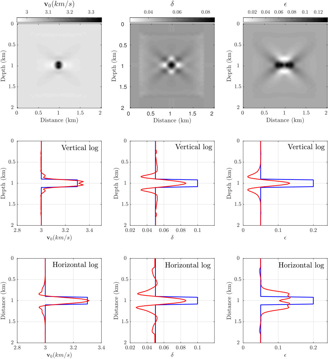 Figure 1
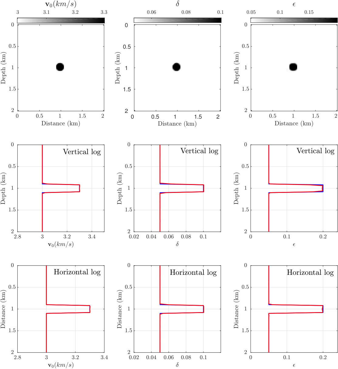 Figure 2
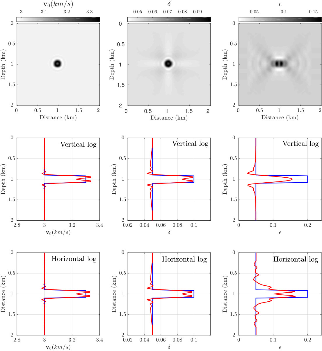 Figure 3
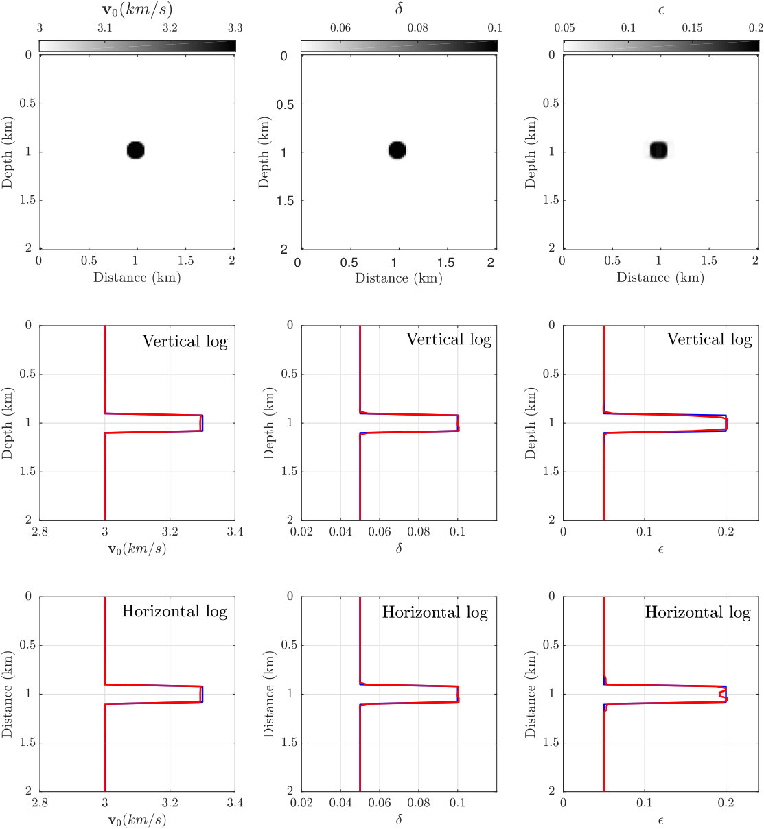 Figure 4
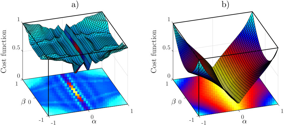 Figure 5
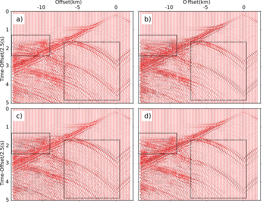 Figure 6
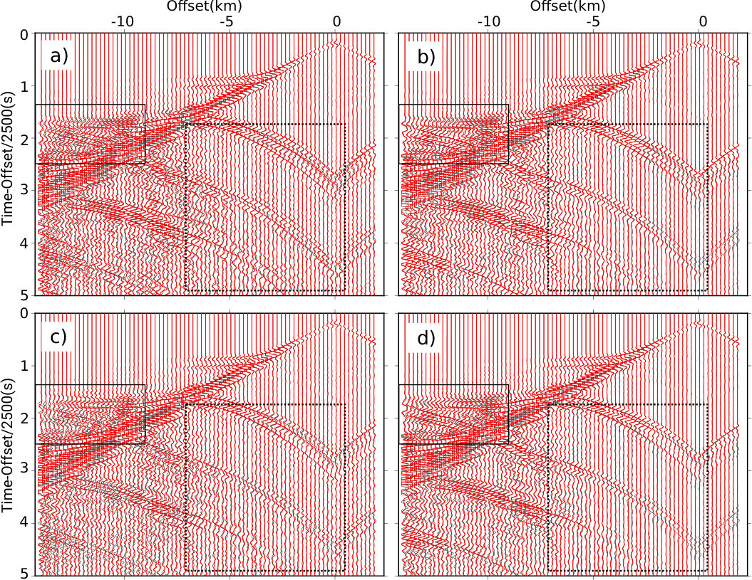 Figure 7
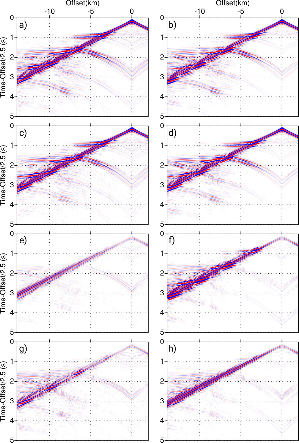 Figure 8
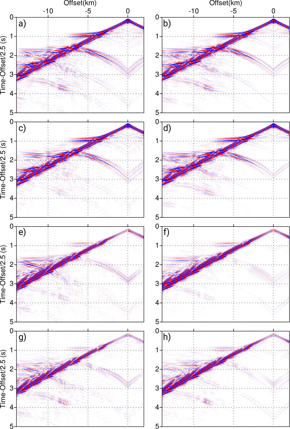 Figure 9
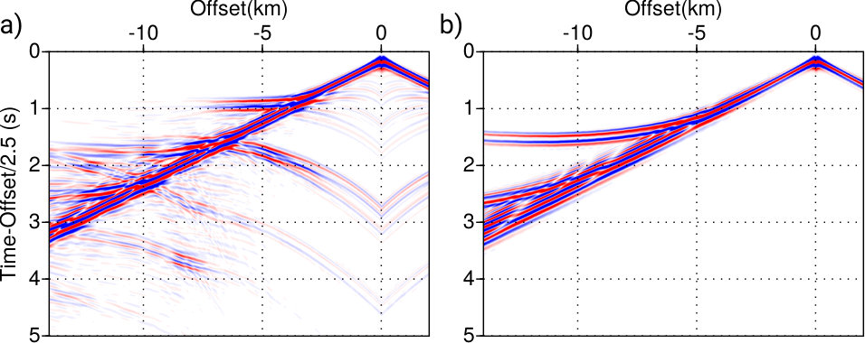 Figure 10
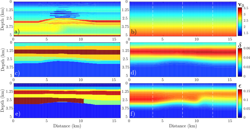 Figure 11
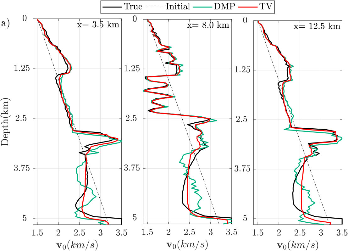 Figure 12
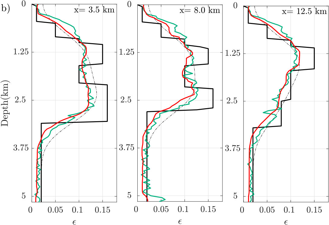 Figure 13
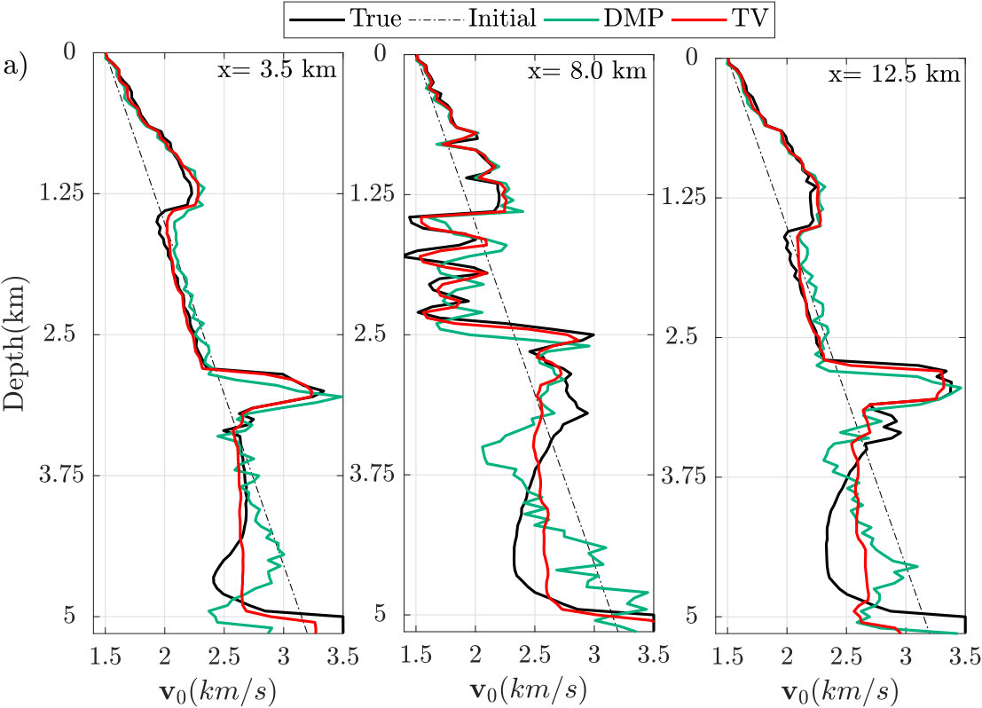 Figure 14
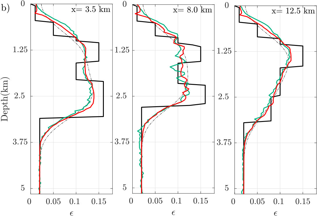 Figure 15
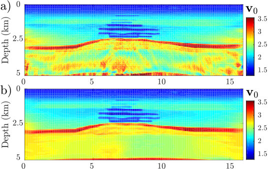 Figure 16
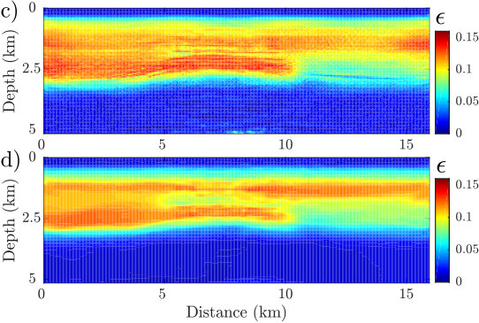 Figure 17
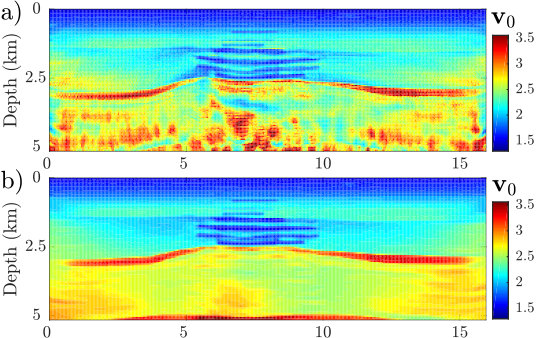 Figure 18
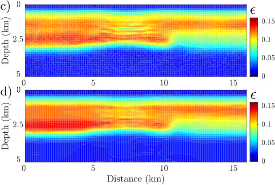 Figure 19
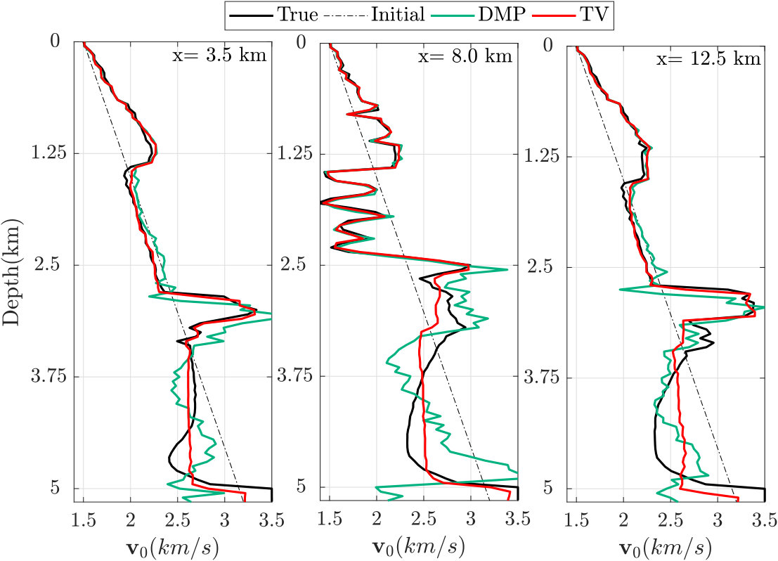 Figure 20
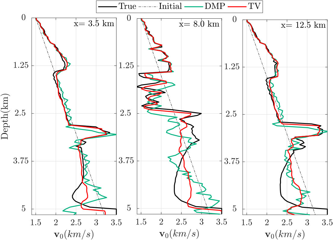 Figure 21
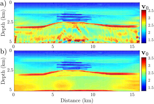 Figure 22
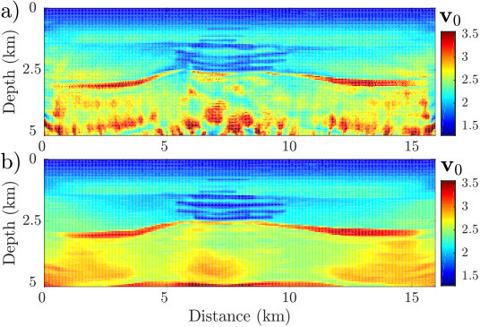 Figure 23
| The corresponding linear system for updating the model | |||
|---|---|---|---|
| a. | p. | p. | |
| p. | a. | p. | |
| p. | p. | a. | |
| p. | a. | a. | |
| a. | a. | p. | |
| a. | p. | a. |
Peer Reviews
No public reviews on file for this paper yet. If you reviewed it on a platform where reviews are public (OpenReview, ICLR, NeurIPS, ICML), you can paste yours below so the community can read it here.
Videos
No videos yet. Explain this paper in a talk, walkthrough, or lecture? Add one.
\lefthead
A PREPRINT - Aghamiry et al. \righthead A PREPRINT - IR-WRI for VTI acoustic medium
ADMM-based multi-parameter wavefield reconstruction inversion in VTI acoustic media with TV regularization
Hossein S. Aghamiry 11footnotemark: 122footnotemark: 2
Ali Gholami 11footnotemark: 1 and Stéphane Operto 22footnotemark: 2
Abstract
Full waveform inversion (FWI) is a nonlinear waveform matching procedure, which suffers from cycle skipping when the initial model is not kinematically-accurate enough. To mitigate cycle skipping, wavefield reconstruction inversion (WRI) extends the inversion search space by computing wavefields with a relaxation of the wave equation in order to fit the data from the first iteration. Then, the subsurface parameters are updated by minimizing the source residuals the relaxation generated. Capitalizing on the wave-equation bilinearity, performing wavefield reconstruction and parameter estimation in alternating mode decomposes WRI into two linear subproblems, which can solved efficiently with the alternating-direction method of multiplier (ADMM), leading to the so-called IR-WRI. Moreover, ADMM provides a suitable framework to implement bound constraints and different types of regularizations and their mixture in IR-WRI. Here, IR-WRI is extended to multiparameter reconstruction for VTI acoustic media. To achieve this goal, we first propose different forms of bilinear VTI acoustic wave equation. We develop more specifically IR-WRI for the one that relies on a parametrisation involving vertical wavespeed and Thomsen’s parameters and . With a toy numerical example, we first show that the radiation patterns of the virtual sources generate similar wavenumber filtering and parameter cross-talks in classical FWI and IR-WRI. Bound constraints and TV regularization in IR-WRI fully remove these undesired effects for an idealized piecewise constant target. We show with a more realistic long-offset case study representative of the North Sea that anisotropic IR-WRI successfully reconstruct the vertical wavespeed starting from a laterally homogeneous model and update the long-wavelengths of the starting model, while a smooth model is used as a passive background model. VTI acoustic IR-WRI can be alternatively performed with subsurface parametrisations involving stiffness or compliance coefficients or normal moveout velocities and parameter (or horizontal velocity).
1 Introduction
Full waveform inversion (FWI) is a waveform matching procedure which provides subsurface model with a wavelength resolution. However, it suffers from cycle skipping when the initial model is not accurate enough according to the lowest available frequency. To mitigate cycle skipping, the search space of frequency-domain FWI can be extended by wavefield reconstruction inversion (WRI) (van Leeuwen and Herrmann,, 2013, 2016). In WRI, the search space is extended with a penalty method to relax the wave-equation constraint at the benefit of the observation equation (i.e., the data fit) during wavefield reconstruction. Then, the subsurface parameters are estimated from the reconstructed wavefields by minimizing the source residuals the relaxation generated. If these two subproblems (wavefield reconstruction and parameter estimation) are solved in alternating mode (van Leeuwen and Herrmann,, 2013) rather than by variable projection (van Leeuwen and Herrmann,, 2016), WRI can be recast as a sequence of two linear subproblems capitalizing on the bilinearity of the scalar Helmholtz equation with respect to the wavefield and the squared slownesses (the Helmholtz equation is linear with respect to the wavefield for a given squared slowness model and is linear with respect to the squared slownesses for a given wavefield).
Aghamiry et al., 2019c improved WRI by replacing the penalty method with the augmented Lagrangian method (Nocedal and Wright,, 2006) and solve it using the alternating-direction method of multipliers (ADMM) (Boyd et al.,, 2010), leading to iteratively-refined WRI (IR-WRI). Although ADMM was originally developed for separable convex problems, the bilinearity of the wave equation makes IR-WRI biconvex, which allows for the use of ADMM as is (Boyd et al.,, 2010, Section 3.1.1). Moreover, a scaled form of ADMM draws clear connection between WRI and IR-WRI in the sense that it shows that IR-WRI reduces to a penalty method in which the right-hand sides (RHSs) in the quadratic objective functions associated with the observation equation and the wave equation are iteratively updated with the running sum of the data and source residuals in iteration (namely, the scaled Lagrange multipliers). This RHS updating, the lacking feature in WRI, efficiently refines the solution of the two linear subproblems when a fixed penalty parameter is used (Aghamiry et al., 2019c, ). Later, Aghamiry et al., 2018b ; Aghamiry et al., 2019b interfaced bound constraints and edge-preserving regularizations with ADMM to manage large-contrast media. Also, to preserve the smooth components of the subsurface when edge preserving regularizations are used, Aghamiry et al., 2018a ; Aghamiry et al., 2019a combine blocky and smooth promoting regularization in the framework of IR-WRI by using infimal convolution of Tikhonov and Total Variation (TV) regularization functions.
IR-WRI was mainly assessed for wavespeed estimation from the scalar Helmholtz equation. The objective of this study is to develop and assess the extension of IR-WRI to multi-parameter reconstruction in VTI acoustic media. To achieve this goal, we first need to review different formulations of the VTI acoustic wave equation and different subsurface parametrisations for which bilinearity of the wave equation is fulfilled, in order to keep the parameter estimation subproblem linear. Since the wavefield reconstruction requires to solve a large and sparse system of linear equations, second-order or fourth-order wave equation for pressure will be favored at the expense of first-order velocity-stress formulations to mitigate the number of unknowns during wavefield reconstruction. However, we stress that different forms of the wave equation can be used to perform wavefield reconstruction and parameter estimation, provided they provide consistent solutions (Gholami et al., 2013b, , Their Appendix A and B).
Also, we will favor subsurface parametrisation involving the vertical wavespeed and the Thomsen’s parameter and at the expense of that involving stiffness coefficients according to the trade-off analysis of Gholami et al., 2013b (, Their Appendix A and B).
When bilinearity of the wave equation is fulfilled, IR-WRI can be extended to multi-parameter estimation following the procedure promoted by Aghamiry et al., 2019b , where TV regularization and bound constraints are efficiently implemented in the parameter-estimation subproblem using variable splitting schemes (Glowinski et al.,, 2017). The splitting procedure allows us to break down the non-differentiable TV regularization problem into two easy-to-solve subproblems: a least-squares quadratic subproblem and a proximity subproblem (Goldstein and Osher,, 2009).
In this study, we perform a first assessment of multi-parameter IR-WRI for and using a toy inclusion example and the more realistic synthetic North Sea case study tackled by Gholami et al., 2013b and Gholami et al., 2013a . With the toy example, we first show that the radiation patterns and the parameter cross-talks have the same effects as in classical FWI when TV regularization is not applied. Then, we show how TV regularization fully removes bandpass filtering and cross-talk effects generated by these radiation patterns for this idealized piecewise constant target. With the North Sea example, we first show the resilience of IR-WRI against cycle skipping when using a crude initial model. The reconstruction of the model is accurate except in the deep smooth part of the subsurface which suffers from a deficit of wide-angle illumination, while the reconstruction of is more challenging and requires additional regularization to keep its update smooth and close to the starting model. However, we manage to update significantly the long-to-intermediate wavelengths of by IR-WRI, unlike Gholami et al., 2013a . Also, comparison between mono-parameter IR-WRI for and multi-parameter IR-WRI for and allows us to gain qualitative insights on the sensitivity of the IR-WRI to in terms of subsurface model quality and data fit.
This paper is organized as follow. We first discuss the bilinearity of the acoustic VTI wave equation as well as its implication on the gradient and the Gauss-Newton Hessian of the parameter-estimation subproblem. From the selected bilinear formulation of the wave equation, we develop bound-constrained TV-regularized IR-WRI for VTI acoustic media parametrized by , and . Third, we assess IR-WRI for VTI acoustic media against the inclusion and North Sea case studies. Finally, we discuss the perspectives of this work.
2 Theory
In this section, we first show that the VTI acoustic wave equations is bilinear with respect to the wavefield and model parameters. Then, we rely on this bilinearity to formulate multi-parameter IR-WRI in VTI acoustic media with bounding constraints and TV regularization.
2.1 Bilinearity of the wave equation: preliminaries
If we write the wave equation in a generic matrix form as
[TABLE]
where is the wave-equation operator, is the wavefield vector, is the source vector, is the subsurface parameter vector, is the number of degrees of freedom in the spatial computational mesh, is the number of wavefield components, is the number of parameter classes, then the wave equation is bilinear if there exists a linear operator such that
[TABLE]
where . Bilinearity is verified when the left-hand side of the wave equation can be decomposed as:
[TABLE]
where is a block matrix, whose blocks of dimension are either 0 or of the form , and matrices , and don’t depend on . The operator denotes a diagonal matrix of coefficients and is the subsurface parameter vector of class . By noting that , the block diagonal structure of allows one to rewrite the term as , where is a block matrix, whose blocks of dimension are either 0 or diagonal with coefficients depending on .
It follows from equation 3 and the above permutation between and that the wave equation can be re-written as
[TABLE]
Moreover, in the framework of multi-parameter analysis, it is worth noting that
[TABLE]
where the left-hand side is the so-called virtual source associated with (Pratt et al.,, 1998) and denotes a column vector whose th component is one while all the others are zeros.
Accordingly, the normal operator , i.e., the Gauss-Newton Hessian of the parameter estimation subproblem in IR-WRI, is formed by the zero-lag correlation of the virtual sources and, hence is extremely sparse. We also point that and its associated normal operator are block diagonals if is diagonal. This means that, if the model parameters are first sorted according to their position in the mesh (fast index) and second according to the parameter class they belong to (slow index), then the diagonal coefficients of the off-diagonal blocks describe the inter-parameter coupling. In the following section, we show the bilinearity of the acoustic VTI wave equation based upon the above matrix manipulations.
2.2 Bilinearity of the acoustic VTI wave equation
2.3 First-order velocity-stress wave equation
We first consider the frequency-domain first-order velocity-stress wave equation in 2D VTI acoustic media (Duveneck et al.,, 2008; Duveneck and Bakker,, 2011; Operto et al.,, 2014)
[TABLE]
where , is the angular frequency, and are the horizontal and vertical particle velocity wavefields, denote the pressure sources, and and are the so-called horizontal and vertical pressure wavefields (Plessix and Cao,, 2011). The subscript is the source index, where denotes the number of sources. The subsurface properties are parametrized by the buoyancy (inverse of density) and the stiffness coefficients . Operators and are finite difference approximation of first order derivative operators with absorbing perfectly matched layer (PML) coefficients (Bérenger,, 1994).
Gathering equation 2.3 for all sources leads to the following matrix equation:
[TABLE]
where is the identity matrix,
[TABLE]
[TABLE]
with
[TABLE]
and analogously for , , , and
[TABLE]
Furthermore,
[TABLE]
Note that, according to the decomposition introduced in the previous section, , , and . Equation 7 is linear in and when the model parameters embedded in and are known. When and are known, this system can be also recast as a new linear system in which the unknowns are the model parameters, thus highlighting the bilinearity of the wave equation. For the th source, the new equations become
[TABLE]
where
[TABLE]
Equations 7 and 9 are equivalent forms of the original equation 2.3. The former expresses the discretized wavefields as the unknowns of a linear system, whose coefficients depend on the known subsurface parameters, while the latter expresses the model parameters as the unknowns of an another linear system, whose coefficients depend on the known wavefields. In the framework of WRI, this bilinearity allows one to recast the waveform inversion problem as two linear subproblems for wavefield reconstruction and parameter estimation, which can be solved efficiently in alternating mode with ADMM (Aghamiry et al., 2019c, ; Aghamiry et al., 2019b, ). In the next section, we show the bilinearity of the second-order frequency-domain wave equation, which may be more convenient to solve with linear algebra methods than the first-order counterpart, since it involves fewer unknowns for a computational domain of given size.
2.4 Second-order wave equation
Following a parsimonious approach (e.g., Operto et al.,, 2007), we eliminate and from equation 2.3 to derive a system of two second-order partial differential equations as
[TABLE]
Equation 10 defines a tri-linear equation with respect to buoyancy, stiffness parameters and pressure wavefields. A tri-linear function is a function of three variables which is linear in one variable when the other two variables are fixed. In this study, we will assume that density is constant and equal to 1 to focus on the estimation of the anisotropic parameters. If heterogeneous density needs to be considered, the second-order wave equation can be recast as a bilinear system if the first-order wave equation is parametrized with compliance coefficients instead of stiffness coefficients (see Appendix A and Vigh et al.,, 2014; Yang et al.,, 2016). Alternatively, the parameter estimation can be performed with the bilinear first-order wave equation, equation 9, while wavefield reconstruction is performed with the second-order wave equation, equation 10, or the fourth-order wave equation reviewed in Appendix C for sake of computational efficiency.
We continue by assuming that the density is constant and equal to 1 and parametrize the VTI equation in terms of vertical wavespeed and Thomsen’s parameters and (Thomsen,, 1986). Accordingly, we rewrite equation 10 as
[TABLE]
where and . We write this linear system in a more compact form as
[TABLE]
where , is defined as in equation 8, and the matrix is given by
[TABLE]
where the model parameters are
[TABLE]
Equation 12 is linear in wavefields when the model parameters are known. When is known, this system can be recast as a linear system in which the unknowns are the model parameters.
[TABLE]
where is given by
[TABLE]
and
[TABLE]
Note that each block of is diagonal. In the next section, we develop multi-parameter acoustic VTI IR-WRI with bound constraints and TV regularization. We give the most general formulation in which all the tree parameter classes , , are optimization parameters (updated by the inversion). However, one may process some of them as passive parameters or update the parameter classes in sequence rather than jointly. In this case, the linear system associated with the parameter estimation subproblem, equation 13, will change. Table 1 presents this system for the different possible configurations.
2.5 ADMM-based acoustic VTI wavefield reconstruction inversion
We consider the following bound-constrained TV-regularized multivariate optimization problem associated with the wave equation described by equation 12:
[TABLE]
where and are, respectively, first-order finite-difference operators in the horizontal and vertical directions with appropriate boundary conditions, is the set of all feasible models bounded by a priori lower bound and upper bound ,
[TABLE]
with denoting the recorded data for the th source, each including samples (the number of receivers), is a linear observation operator which samples the wavefields at the receiver positions. Here, we assume that the sampling operator is identical across all sources (stationary-recording acquisitions). However, one may used a specific operator for each source.
We solve this constrained optimization problem with ADMM (Boyd et al.,, 2010; Aghamiry et al., 2019b, ), an augmented Lagrangian method with operator splitting, leading to the following saddle point problem
[TABLE]
where denotes the Frobenius norm of , are penalty parameters and and are the Lagrange multipliers (dual variables).
The last two lines of Equation 15 shows that the augmented Lagrangian function combines a Lagrangian function (left terms) and a penalty function (right terms). Also, scaling the Lagrange multipliers by the penalty parameters, and , allows us to recast the augmented Lagrangian function in a more convenient form (Boyd et al.,, 2010, Section 3.1.1)
[TABLE]
where the scaled dual variables have been injected in the penalty functions.
In the WRI framework, the augmented Lagrangian method provides an efficient and easy-to-tune optimization scheme that extends the parameter search space by introducing a significant relaxation of the wave equation at the benefit of the observation equation during the early iterations, while satisfying the two equations at the convergence point. We solve the saddle point problem, equation 16, with the method of multiplier, in which the primal variables, and , and the dual variables, and , are updated in alternating mode. The dual problem is iteratively solved with basic gradient ascent steps. Accordingly, we immediately deduce from equation 16 that the scaled dual variables and are formed by the running sum of the constraint violations (the data and source residuals) in iterations. They update the RHSs (the data and the sources) of the quadratic penalty functions in equation 16 to refine the primal variables and at a given iteration from the residual source and data errors (this RHS updating is a well known procedure to iteratively refine solutions of ill-posed linear inverse problems). The bi-variate primal problem, equation 14, is biconvex due to the bilinearity of the wave equation highlighted in the previous section. Therefore, it can be broken down into two linear subproblems for and , which can be solved efficiently in alternating mode with ADMM after noting that the TV regularizer is convex (Aghamiry et al., 2019b, ).
As pointed out by Aghamiry et al., 2019c , a key advantage of augmented Lagrangian methods compared to penalty methods is that fixed penalty parameters and can be used in iterations, because the Lagrange multipliers progressively correct for the constraint violations generated by the penalty terms through the above mentioned RHS updating.
Starting from an initial model and zero-valued dual variables, the th ADMM iteration embeds the following steps (see Appendix B for the complete development):
2.5.1 Step 1: The primal wavefield reconstructions.
Build regularized wavefields by solving the following multi-RHS system of linear equations with direct or iterative methods suitable for sparse matrices:
[TABLE]
By choosing a small value of , the reconstructed wavefields closely fit the observations during the early iterations, while only weakly satisfying the wave equation. Problem 17 can be also interpreted as an extrapolation problem to reconstruct , when the observation equation (i.e. ) is augmented with the wave equation.
To mitigate the computational burden of the wavefield reconstruction, we solve equation 17 with a fourth-order wave equation operator following the parsimonious approach of Operto et al., (2014), while the subsequent model estimation subproblem relies on the bilinear wave equation provided in equation 11. The elimination procedure allowing to transform the system of two second-order wave equations for and , equation 11, into a fourth-order wave equation for coupled with the closed-form expression of as a function of is reviewed in Appendix C.
2.5.2 Step 2: The primal model estimation.
The reconstructed wavefields, equation 17, are injected in the linearized equation 13 to update the subsurface parameters by solving the following system of linear equations:
[TABLE]
where
[TABLE]
In equation 18, and are auxiliary primal variables, which have been introduced to solve the bound-constrained TV-regularized parameter estimation subproblem with the split Bregman method (Appendix B). The vectors and are the corresponding dual variables. These auxiliary primal and dual variables are initialized to during the first ADMM iteration.
The operator is a diagonal weighting matrix defined as
[TABLE]
where control the relative weights assigned to the bound constraints applied on the three parameter classes. Note that the bound constraints introduce also a damping (DMP) or zero-order Tikhonov regularization in the Hessian of equation 18.
In the same way, is a diagonal matrix defined as
[TABLE]
where
[TABLE]
and control the soft thresholding that is performed by the TV regularizer, equation 23. We remind that augmented Lagrangian methods seek to strictly satisfy the constraints at the convergence point only, not at each iteration. Therefore, the relative values of these penalty parameters have a significant impact upon the path followed by the inversion to converge toward this convergence point.
2.5.3 Step 3: The TV primal update.
Update the TV primal variable via a TV proximity operator. Set
[TABLE]
then
[TABLE]
where
[TABLE]
and denotes the Hadamard (component-wise) product of and . Also, the power of 2 indicates the Hadamard product of with itself, i.e. .
2.5.4 Step 4: The bounding constraint primal update.
Update the primal variable via a projection operator, which has the following component-wise form
[TABLE]
where the projection operator is given by
[TABLE]
2.5.5 Step 5: Dual updates.
Update the scaled dual variables with gradient ascent steps
[TABLE]
2.5.6 Step 6: Check the stopping condition.
Exit if the preset stopping conditions are satisfied else go to step 1. We will describe the stopping criteria of iterations in the following ”Numerical example” section for each numerical example
2.6 Hyperparameter tuning
We tune the different penalty parameters by extending the procedure reviewed by Aghamiry et al., 2019b ; Aghamiry et al., 2019a to multiparameter reconstruction.
We start from the last subproblem of the splitting procedure and set the penalty parameters contained in . These hyperparameters control the soft thresholding performed by the TV regularization, equation 22. We set , where the subscript denotes the parameter class (, , ). This tuning can be refined by using a different thresholding percentage for each parameter class adaptively during iterations or according to prior knowledge of the geological structure, coming from well logs for example. Also, we use the same weight for the damping regularization associated with the bound constraints and the TV regularization: .
Then, we select as a percentage of the mean absolute value of the diagonal coefficients of during the parameter estimation subproblem, equation 18. This percentage is set according to the weight that we want to assign to the TV regularization and the bound constraints relative to the wave equation constraint during the parameter estimation. Parameter may be increased during iterations to reduce the weight of TV regularization and bound constraints near the convergence point. We found this adaptation useful when we start from very crude initial models. Finally, we set such that is a small fraction of the highest eigenvalue of the normal operator during the wavefield reconstruction subproblem, equation 17, according to the criterion proposed by van Leeuwen and Herrmann, (2016). In all the numerical tests, we use and for noiseless and noisy data, respectively. This tuning of is indeed important because it controls the extension of the search space. A too high value of reduces the weight of during the wavefield reconstruction and makes IR-WRI behave like a reduced approach. Conversely, using a small value for fosters data fitting and expends the search space accordingly. However, a too small value can lead to a prohibitively high number of iterations of the augmented Lagrangian method before the wave equation constraint is fulfilled with sufficient accuracy. Moreover, when data are contaminated by noise, a too small value for will make the wavefield reconstruction over-fit the data and drive the algorithm to be a poor minimizer. We always use as a fixed percentage of in iterations.
3 Numerical examples
3.1 Inclusion test
We first assess multi-parameter IR-WRI with a simple inclusion example for noiseless data. The experimental setup in terms of model, acquisition geometry and frequency selection is identical to that used by Gholami et al., 2013b . The vertical velocity and the Thomsen’s parameters and are 3 km/s, 0.05 and 0.05, respectively, in the homogeneous background model and 3.3 km/s, 0.1 and 0.2, respectively, in the inclusion of radius 100 m. Nine frequencies between 4.8 Hz and 19.5 Hz are processed simultaneously during IR-WRI and a maximum of 25 iterations is used as stopping criterion for iterations. An ideal fixed-spread acquisition is used, where 64 sources and 320 receivers surround the inclusion, hence providing a complete angular illumination of the target.
Although we use as optimization parameters during our inversions, we show the reconstructed models under the form of , and for comparison with the results of Gholami et al., 2013b . Note that the radiation patterns of the parametrisation are scaled versions of those of the parametrisation: namely, they exhibit the same amplitude variation with scattering angle, with however different amplitudes. This means that, for an equivalent regularization and parameter scaling, we expect similar resolution and trade-off effects with these two parametrisations. Note that is provided in km/s in our inversion such that the order of magnitude of is of the order of and .
We start with bound-constrained IR-WRI with damping (DMP) regularization only ( in equation 18) and perform three independent mono-parameter reconstructions for , and , respectively. For each mono-parameter inversion, the true model associated with the optimization parameter contains the inclusion, while the true models associated with the two passive parameters are homogeneous (Fig. 1). For all three inversions, the starting models are the true homogeneous background models. In other words, the data residuals contain only the footprint of the mono-parameter inclusion to be reconstructed. This test is used to assess the intrinsic resolution of IR-WRI for each parameter reconstruction, independently from the cross-talk issue (Gholami et al., 2013b, ). It is reminded that this intrinsic resolution is controlled by the frequency bandwidth, the angular illumination provided by the acquisition geometry and the radiation pattern of the optimization parameter in the chosen subsurface parametrisation. As this test fits the linear regime of classical FWI, we obtain results (Fig. 1) very similar to those obtained by Gholami et al., 2013b (, Their Fig. 9), where the shape of the reconstructed inclusions is controlled by the radiation pattern of the associated parameter. The reader is referred to Gholami et al., 2013b for a detailed analysis of these radiation patterns.
Then, we perform the joint reconstruction of , and , when the true model contains an inclusion for each parameter class (Fig. 2). With our parameter scaling and subsurface parametrisation, , and are reconstructed with well balanced amplitudes compared to the results of Gholami et al., 2013b (, Their Fig. 10), where has a dominant imprint in the inversion. Comparing the models reconstructed by the mono-parameter and multi-parameter inversions highlights however the wavenumber leakage generated by parameter cross-talks (Figs. 1 and 2).
Then, we complement DMP regularization with TV regularization during bound-constrained IR-WRI for the above mono-parameter and multi-parameter experiments (Figs. 3 and 4). The results show how TV regularization contributes to remove the wavenumber filtering performed by radiation patterns (compare for example Figs. 1 and 3) as well as the cross-talk artifacts during the multi-parameter inversion (compare Figs. 2 and 4). Although this toy example has been designed with a piecewise constant model which is well suited for TV regularization, yet it highlights the potential role of TV regularization to mitigate the ill-posedness of FWI resulting from incomplete wavenumber coverage and parameter trade-off.
3.2 Synthetic North Sea case study
3.2.1 Experimental setup
We consider now a more realistic shallow-water model representative of the North Sea (Munns,, 1985). The reader is also referred to Gholami et al., 2013a for an application of acoustic VTI FWI on this model. The true model and the initial (starting) models for , and are shown in Fig. 5. The subsurface model is formed by soft sediments in the upper part, a pile of low-velocity gas layers above a chalk reservoir, the top of which is indicated by a sharp positive velocity contrast at around 2.5 km depth, and a flat reflector at 5 km depth (Fig. 5a). The initial model is laterally homogeneous with velocity linearly increasing with depth between 1.5 to 3.2 km/s (Fig. 5b), while the and initial models are Gaussian filtered version of the true models. Note that our initial/background , and models are cruder than those used by Gholami et al., 2013a .
The fixed-spread surface acquisition consists of 80 (reciprocal) explosive sources spaced 200 m apart at 75 m depth on the sea bottom and 320 (reciprocal) hydrophone receivers spaced 50 m apart at 25 m depth. Accordingly, the pressure wavefield is considered for the acoustic VTI inversion. A free-surface boundary condition is used on top of the grid and the source signature is a Ricker wavelet with a 10 Hz dominant frequency. We compute the recorded data in the true models (Figs. 5a,c,e) with the forward modelling engine described in Appendix C. During IR-WRI, we use the same forward engine to compute the modelled data according to an inverse crime procedure. Common-shot gathers computed in the true model and in the initial model for a shot located at 14 km are shown in Fig. 7. The seismograms computed in the true model are dominated by the direct wave, the diving waves from the sedimentary overburden, complex packages of pre- and post-critical reflections from the gas layers, the top of the reservoir and the deep reflector. The refracted wave from the deep reflector is recorded at a secondary arrival between -14km and -10km offset in Fig. 7a. Also, energetic reverberating P-wave reflections are generated by the wave guide formed by the shallow water layer and the weathering layer. They take the form of leaking modes with phase velocities higher than the water wave speed (Operto and Miniussi,, 2018). The seismograms computed in the starting model mainly show the direct wave and the diving waves, these latter being highly cycle skipped relative to those computed in the true model.
We perform both mono-parameter IR-WRI for and multi-parameter IR-WRI for and . In both cases, we compare the results that are obtained when bound-constrained IR-WRI is performed with DMP regularization only () and with DMP + TV regularization. When is involved as an optimization parameter, we had to introduce an additional regularization term in the parameter-estimation subproblem, equation 40a, in order to force the updates of to be smooth and close to . The background models used for the passive anisotropic parameters (either and or alone) are the smooth models (Fig. 5d,f), which means that the IR-WRI results will be impacted upon by the smoothness of the passive parameters.
We perform IR-WRI with small batches of two frequencies with one frequency overlap between two consecutive batches, moving from the low frequencies to the higher ones according to a classical frequency continuation strategy. The starting and final frequencies are 3 Hz and 15 Hz and the sampling interval in one batch is 0.5 Hz. The stopping criterion for iterations and for each batch is given by or
[TABLE]
where denotes the maximum iteration count, =1e-3, and =1e-5 for noiseless data and =1e-3 , = noise level of batch for noisy data.
We perform three paths through the frequency batches to improve the IR-WRI results, using the final model of one path as the initial model of the next one (these cycles can be viewed as outer iterations of IR-WRI). The starting and finishing frequencies of the paths are [3, 6], [4, 8.5], [6, 15] Hz respectively, where the first element of each pair shows the starting frequency and the second one is the finishing frequency.
3.2.2 Convexity and sensitivity analysis
Before discussing the IR-WRI results, we illustrate how WRI extends the search space of FWI for the North Sea case study. For this purpose, we compare the shape of the FWI misfit function with that of the parameter-estimation WRI subproblem for the 3 Hz frequency and for a series of and models that are generated according to
[TABLE]
where and denote the true and the initial models, respectively (Fig. 5a,b) and . Similarly, and are the true and the initial models, respectively (Fig. 5e,f) and . Finally, we use the true model (Fig. 5c) to generate the recorded data and the smoothed version (Fig. 5d) as a passive parameter to evaluate the misfit function. The misfit functions of the classical reduced-approach FWI as well as that of WRI are shown in Fig. 6. The WRI misfit function is convex, while that of FWI exhibits spurious local minima along both the and dimensions. Also, the sensitivity of the misfit function to is much higher than that of for the considered range of models as already pointed out by Gholami et al., 2013b , Gholami et al., 2013a and Cheng et al., (2016, Their Fig. 2). The weaker sensitivity of the misfit function to makes the joint update of and challenging.
3.2.3 Mono-parameter IR-WRI
We start with mono-parameter bound-constrained IR-WRI when is the optimization parameter and and are passive parameters. We first consider noiseless data.
The final models inferred from bound-constrained IR-WRI with DMP regularization only and DMP+TV regularizations are shown in Fig. 8. Also, direct comparisons between the logs extracted from the true model, the initial model, and the IR-WRI models at , and are shown in Fig. 9. Although the crude initial model and the smooth and passive models, the shallow sedimentary part and the gas layers are fairly well reconstructed with the two regularization settings. The main differences are shown at the reservoir level and below. Without TV regularization, the reconstruction at the reservoir level is quite noisy and the inversion fails to reconstruct the smoothly-decreasing velocity below the reservoir due to the lack of diving wave illumination at these depths. This in turn prevents the focusing of the deep reflector at 5 km depth by migration of the associated short-spread reflections. When TV regularization is used, IR-WRI provides a more accurate and cleaner image of the reservoir and better reconstructs the sharp contrast on top of it. It also reconstructs the deep reflector at the correct depth in the central part of the model, while the TV regularization has replaced the smoothly-decreasing velocities below the reservoir by a piecewise constant layer with a mean velocity (Fig. 9).
To generate more realistic test, we add random noise with Gaussian distribution to the data with SNR=10 db and re-run the mono-parameter bound-constrained IR-WRI with DMP and TV regularizations (Fig. 10). The direct comparison between the true model, the initial model and the IR-WRI models of Fig. 10 at distances , and are shown in Fig. 11. The noise degrades the reconstruction of the gas layers both in terms of velocity amplitudes and positioning in depth when only DMP regularization is used. Also, the sharp reflector on top of the reservoir is now unfocused and mis-positioned in depth accordingly (Fig. 11). The TV regularization significantly reduces these amplitude and mis-positioning errors (Figs. 10b and 11) and hence produces models which are much more consistent with those obtained for noiseless data (Figs. 8b and 9).
To assess how the differences between the velocity models shown in Fig. 8 impact waveform match, we compute time-domain seismograms in these models as well as the differences with those computed in the true model (Figs. 12 and 13). The time-domain seismograms and the residuals shown in Fig. 12 give an overall vision of the achieved data fit, while the direct comparison between the recorded and modelled seismograms shown in Fig. 13 allow for a more detailed assessment of the waveform match for a specific arrival.
A first conclusion is that, for all of the models shown in Fig. 8, the main arrivals, namely those which have a leading role in the reconstruction of the subsurface model (diving waves, pre- and post-critical reflections), are not cycle skipped relative to those computed in the true model. We note however more significant residuals for the reverberating guided waves when TV regularization is used. These mismatches were generated by small wavespeed errors generated in the shallow part of the model by the TV regularization. These artifacts can be probably corrected by deactivating or decreasing the weight of the TV regularization locally. For noiseless data, the direct comparison between the seismograms computed in the true model and in the reconstructed ones show how the DMP+TV regularization improves the waveform match both at pre- and post-critical incidences relative to the DMP regularization alone (Fig. 13a,b). For noisy data, the data fit is slightly degraded by noise when DMP regularization is used, while the TV regularization produces a data fit which is more consistent with that obtained with noiseless data (Compare Figs. 13a and 13c for DMP regularization, and Figs. 13b and 13d for DMP+TV regularization). It is striking to see the strong impact of noise on the quality of the reconstruction when DMP regularization is used (compare Figs. 8a and 10a, and Figs. 9 and 11, green curves), compared to its more moderate impact on the data fit (Compare Figs. 13a and 13c). This highlights the ill-posedness of the FWI, which is nicely mitigated by the prior injected by the TV regularization as illustrated by the consistency of the models inferred from noiseless and noisy data (Compare Figs. 13b and 13b).
3.2.4 Multi-parameter IR-WRI
We continue with multi-parameter bound-constrained IR-WRI when and are optimization parameters and is a passive parameter. As for the mono-parameter inversion, we start with noiseless data. The final and models inferred from bound-constrained IR-WRI with DMP and DMP+TV regularizations are shown in Fig. 14. The direct comparisons between the logs extracted from the true model, the initial model, the bound constrained IR-WRI models with DMP and DMP+TV regularization at , and are shown in Fig. 15a, and the same comparisons for are depicted in Fig. 15b. Compared to the mono-parameter inversion results, involving as an optimization parameter clearly improves the reconstruction at the reservoir level down to around 3 km depth (compare Figs. 8 and 14a,b). The long to intermediate wavelengths of the model are primarily updated according to the radiation pattern of this parameter in the () parametrisation. The main effect of TV regularization relative to DMP regularization is to remove high-frequency noise from the model (Fig. 15b).
The time-domain seismograms computed in the multi-parameter models inferred from bound-constrained IR-WRI when DMP and DMP+TV regularizations are used are shown in Fig. 18. The direct comparison between the recorded and modelled seismograms is shown in Fig. 19a,b. Clearly, using both and as optimization parameters allows us to better conciliate the fit of the pre- and post-critical reflections (Compare Figs. 13a and 19a for DMP regularization, and Figs. 13b and 19b for DMP+TV regularization). With noiseless data, DMP regularization is enough to achieve a high-fidelity data fit, which looks better than that obtained with DMP+TV regularization (Compare Figs. 19a and 19b).
We repeat now the joint inversion when data are contaminated by Gaussian random noise with a SNR=10 db. The final and models inferred from bound-constrained IR-WRI with DMP and DMP+TV regularization are shown in Fig. 16. Direct comparisons along logs extracted from the true models, the initial models, and the models inferred from the bound constrained multi-parameter IR-WRI with DMP and DMP+TV regularization at , and are shown in Fig. 17. For the reconstruction, a trend similar to that shown for the mono-parameter inversion is shown, with a more significant impact of the noise on the velocity model reconstructed with DMP regularization compared to the one reconstructed with DMP+TV regularization (Compare Figs. 14 and 16). As expected, the impact of noise is more significant on the second-order model, even when TV regularization is used, in the sense that the estimated perturbations of the initial model have smaller amplitudes compared to the noiseless case (Fig. 17b).
The time-domain seismograms are shown in Figs. 18 and 19c,d. The data fit obtained with DMP regularization has been significantly degraded compared to that obtained with noiseless data (compare Figs. 19a and 19c), while the data fit obtained with DMP+TV regularization is more consistent with noiseless and noisy data (compare Figs. 19b and 19d). This is consistent with the previous conclusions drawn from the mono-parameter inversion.
4 Discussion
We have extended the ADMM-based wavefield reconstruction inversion method (IR-WRI), originally developed for mono-parameter wavespeed reconstruction (Aghamiry et al., 2019c, ; Aghamiry et al., 2019b, ), to multi-parameter inversion in VTI acoustic media. We have first discussed which formulations of the VTI acoustic wave equation are bilinear in wavefield and subsurface parameters. First-order velocity stress form is often more convenient than the second-order counterpart to fullfil bilinearity, in particular if density (or buoyancy) is an optimization parameter. However, it may be not the most convenient one for frequency-domain wavefield reconstruction as the size of the linear system to be solved scales to the number of wavefield components. To bypass this issue, wavefield reconstruction and parameter estimation can be performed with different wave equations, provided they give consistent solutions (Gholami et al., 2013a and this study).
Bilinearity allows us to recast the parameter estimation subproblem as a linear subproblem and hence the waveform inversion as a biconvex problem. Although ADMM has been originally developed to solve distributed convex problems, it can be used as is to solve biconvex problem (Boyd et al.,, 2010). From the mathematical viewpoint, biconvex problems should have superior convergence properties compared to fully nonconvex problem (this discussion is out of the scope of this study but we refer the interested reader to Benning et al.,, 2015). Alternatively, ADMM-like optimization can be used to perform IR-WRI heuristically without bilinear wave equation, hence keeping the parameter estimation subproblem, equation 40a, nonlinear. Accordingly, equation 40a would be solved with a Newton algorithm rather than with a Gauss-Newton one. This nonlinear updating of the parameters may however require several inner Newton iterations per IR-WRI cycle, while Aghamiry et al., 2019c showed that one inner Gauss-Newton iteration without any line search was providing the most efficient convergence of IR-WRI when bilinearity is fulfilled.
Indeed, the bilinearity specification limits the choice of subsurface parametrisation for parameter estimation. In the general case of triclinic elastodynamic equations, a subsurface parametrisation involving buoyancy and stiffness or compliance coefficients will be the most natural ones, as they correspond to the coefficients of the equation of motion and the Hooke’s law. In the particular case of the VTI acoustic wave equation, we have developed a bilinear wave equation whose coefficients depend on the vertival wavespeed and the Thomsen’s parameters and . Although and are coupled at wide scattering angles, the parametrisation was promoted by Gholami et al., 2013b and Gholami et al., 2013a because the dominant parameter has a radiation pattern which doesn’t depend on the scatteting angle, and hence can be reconstructed with a high resolution from wide-azimuth long-offset data. The counterpart is that updating the long wavelengths of the secondary parameter is challenging and requires so far a crude initial guess of its long wavelengths (Fig. 5e,f), which can be used as prior to regularize the update. Comparing the results of IR-WRI when is used as a passive parameter and as an optimization parameter shows that the sensitivity of the inversion to remains small provided that a reasonable guess of its long wavelengths are provided in the starting model (for the models, compare Figs. 8-10 and Figs. 14-16; for the data fit, compare Fig. 13 and Fig. 19). This limited sensitivity of FWI to the short-to-intermediate wavelengths of in the prompted for example Debens et al., (2015) to estimate a crude background model with a coarse parametrisation by global optimization.
Among the alternative parametrisations proposed for VTI acoustic FWI, Plessix and Cao, (2011) proposed the or the parametrisations for long-offset acquisition, while Alkhalifah and Plessix, (2014) promoted the parametrisation, where is the so-called NMO velocity, is the horizontal velocity and represents the anellipticity of the anisotropy. For the parametrisation promoted by Plessix and Cao, (2011), the VTI equation developed by Zhou H., (2006) given by
[TABLE]
is bilinear in wavefields and parameters , where and . Note that if is assumed to be smooth, the above equation can be approximated as
[TABLE]
which is bilinear in wavefields and parameters . This implies that can be involved as an optimization parameter if necessary. Note that, if this smoothness approximation is used to update the parameters during the primal problem, the modelled data and the source residuals can be solved with the exact equation to update the dual variables with more accuracy. For the parametrisations (Alkhalifah and Plessix,, 2014), according to Zhou H., (2006) the VTI equations with smooth can be written as
[TABLE]
which is bilinear in wavefields and parameters
5 Conclusion
We have shown that ADMM-based IR-WRI can be extended to multi-parameter reconstruction for VTI acoustic media. The gradient of the misfit function for the parameter estimation subproblem involves the so-called virtual sources, which carry out the effect of the parameter-dependent radiation patterns. This suggests that, although IR-WRI extends the search-space of FWI to mitigate cycle skipping, it is impacted by ill-posedness associated with parameter cross-talk and incomplete angular illumination as classical FWI. We have verified this statement with a toy numerical example for which we have reproduced the same pathologies in terms of resolution and parameter cross-talks as those produced by classical FWI during a former study. We have illustrated how equipping IR-WRI with bound constraints and TV regularization fully remove the ill-posedness effects for this idealized numerical example. We have provided some guidelines to design bilinear wave equation of different order for different subsurface parametrisations. Although bilinearity puts some limitations on the choice of the subsurface parametrisation, it recasts the parameter estimation subproblem as a quadratic optimization problem, which can be solved efficiently with Gauss-Newton algorithm. Application on the long-offset synthetic case study representative of the North Sea has shown how IR-WRI can be started from a crude laterally-homogeneous vertical velocity model without impacting the inversion with cycle skipping, when a smooth parameter is used as a passive background model. However, a smooth initial model, albeit quite crude, is necessary to guarantee the convergence of the method to a good solution, either when is used as a passive or as an optimization parameter. For this case study where the low velocity gas layers and the smooth medium below the reservoir suffer from a deficit illumination of diving waves, the TV regularization plays a key role to mitigate the ill-posedness.
6 Acknowledgments
This study was partially funded by the SEISCOPE consortium (http://seiscope2.osug.fr), sponsored by AKERBP, CGG, CHEVRON, EQUINOR, EXXON-MOBIL, JGI, PETROBRAS, SCHLUMBERGER, SHELL, SINOPEC and TOTAL. This study was granted access to the HPC resources of SIGAMM infrastructure (http://crimson.oca.eu), hosted by Observatoire de la Côte d’Azur and which is supported by the Provence-Alpes Côte d’Azur region, and the HPC resources of CINES/IDRIS/TGCC under the allocation 0596 made by GENCI.
\append
First and second-order wave equation with compliance notation We consider the frequency-domain first-order velocity-stress equation in 2D VTI acoustic media with compliance notation as
[TABLE]
where are the compliance coefficients, and the other notations are defined after equation 2.3. Gathering equation 6 for all sources results in the following matrix equation:
[TABLE]
where
[TABLE]
and the other notations are defined in equation 7. Equation 32 is linear in and when the model parameters embedded in and are known. When and are known, this system can be recast as a new linear system in which the unknowns are the model parameters, and hence the bilinearity of the wave equation. For the th source, the new equation becomes
[TABLE]
where
[TABLE]
To develop the second-order wave equation, we eliminate and from equation 6. We obtain the following equation
[TABLE]
which is bilinear with respect to buoyancy, compliance parameters and pressure wavefields. With known buoyancy and compliance parameters, we get the following linear system to estimate wavefields for all sources
[TABLE]
where is given by
[TABLE]
and
[TABLE]
and is defined in equation 8. When is known, this system can also be recast as a new linear system in which the unknowns are the model parameters as
[TABLE]
where is given by
[TABLE]
and
[TABLE]
\append
Solving the optimization problem, equation 16, with ADMM Starting from an initial model , and setting the dual variables and equal to zero, the th ADMM iteration for solving equation 16 reads as (see Aghamiry et al., 2019c, ; Aghamiry et al., 2019b, ; Aghamiry et al., 2019d, , for more details)
[TABLE]
where
[TABLE]
and
[TABLE]
The regularized wavefields are the minimizers of the quadratic cost function , equation 38, where , and are kept fixed. Zeroing the derivative of gives the wavefields as the solution of a linear system of equations defined by equation 17 (step 1 of the algorithm). The regularized wavefields are then introduced as passive quantities in the cost function , equation 39, which is minimized to estimate over the desired set . We solve this minimization subproblem with the splitting techniques. Accordingly, we introduce the auxiliary primal variables and to decouple the and terms and split the parameter estimation subproblem into three sub-steps for , and (Goldstein and Osher,, 2009; Aghamiry et al., 2019b, ):
[TABLE]
where is defined in equation 19,
[TABLE]
, and are diagonal matrices defined in equation 20 and 21, respectively.
From the linearized equation 13, the subproblem for , equation 40a, can be written as
[TABLE]
where the diagonal weighting matrix is defined as
[TABLE]
Equation 42 is now quadratic and admits a closed form solution as given in equation 18 (step 2 of the algorithm).
The only remaining tasks consist in determining the auxiliary primal variables , equations 40b,c, and the auxiliary dual variables . They are initialized to 0 and are updated as follows: The primal variables is updated through a TV proximity operator, which admits a closed form solution given by equation 22 (see Combettes and Pesquet,, 2011) (step 3 of the algorithm). The primal variable is updated by a projection operator, which also admits a closed form solution given by equation 24 (step 4 of the algorithm). Finally, the duals are updated according to gradient ascend steps (step 5 of the algorithm)
[TABLE]
\append
Using fourth-order equation for wavefield reconstruction (Step 1 of the algorithm) The wavefield reconstruction subproblem, equation 17, can be written as the following over-determined system
[TABLE]
where is the sampling operator of each component of the wavefield at receiver positions and (the coefficient results because the (isotropic) pressure wavefield recorded in the water is given by ). We can eliminate from the equation 6 to develop a fourth-order partial-differential equation for and then update from its explicit expression as a function of without any computational burden.
By multiplying the second row of equation 6 by and taking the difference with the first row, we find
[TABLE]
where . The second equation of 6 provides us the closed-form expression of as a function of
[TABLE]
where
[TABLE]
Injecting equation 47 into the first equation of 6 leads to the over-determined system satisfied by
[TABLE]
So, instead of solving the linear system 6 to update , is updated by solving the linear system 6 and then is updated using 47 without significant computational overhead. The wave equation operator in equation 47 has been broken down into an elliptic wave equation operator and anelliptic correction term (the term of related to , equation 47). The former can be accurately discretized with the 9-point finite-difference method of Chen et al., (2013), while the anelliptic term can be discretized with a basic second-order accurate 5-point stencil without generating significant inaccuracies in the modelling (Operto et al.,, 2014).
The reference list from the paper itself. Each links out to its DOI / PubMed record.
- 1(1) Aghamiry, H., A. Gholami, and S. Operto, 2018 a, Hybrid tikhonov + total-variation regularization for imaging large-contrast media by full-waveform inversion: Expanded Abstracts, 88 th Annual SEG Meeting (Anaheim), 1253–1257.
- 2(2) ——–, 2018 b, Imaging contrasted media with total variation constrained full waveform inversion and split Bregman iterations: Presented at the Expanded Abstracts, 80 th Annual EAGE Meeting (Copenhagen).
- 3(3) ——–, 2019 a, Compound Regularization of Full-Waveform Inversion for Imaging Piecewise Media: ar Xiv:1903.04405.
- 4(4) ——–, 2019 b, Implementing bound constraints and total-variation regularization in extended full waveform inversion with the alternating direction method of multiplier: application to large contrast media: Geophysical Journal International, 218 , 855–872.
- 5(5) ——–, 2019 c, Improving full-waveform inversion by wavefield reconstruction with alternating direction method of multipliers: Geophysics, 84(1) , R 139–R 162.
- 6(6) ——–, 2019 d, Multi-parameter ADMM-based wavefield reconstruction inversion in VTI acoustic media: Presented at the 81 th Annual EAGE Meeting (London).
- 7Alkhalifah and Plessix, (2014) Alkhalifah, T. and R. Plessix, 2014, A recipe for practical full-waveform inversion in anisotropic media: An analytical parameter resolution study: Geophysics, 79 , R 91–R 101.
- 8Benning et al., (2015) Benning, M., F. Knoll, C.-B. Schönlieb, and T. Valkonen, 2015, Preconditioned admm with nonlinear operator constraint: IFIP Conference on System Modeling and Optimization, 117–126.