A Solvable Two-dimensional Optimal Stopping Problem in the Presence of Ambiguity
S\"oren Christensen, Luis H. R. Alvarez E

TL;DR
This paper explores how ambiguity influences optimal stopping times in a multidimensional setting, revealing that ambiguity affects both growth and discount rates, which is a novel insight not present in one-dimensional models.
Contribution
It introduces a multidimensional model showing that ambiguity impacts both growth and discount rates, providing a new perspective on optimal timing under uncertainty.
Findings
Ambiguity affects the rate of growth of underlying processes.
Ambiguity influences the discount rate in the model.
Multidimensional setting reveals effects not seen in one-dimensional models.
Abstract
According to conventional wisdom, ambiguity accelerates optimal timing by decreasing the value of waiting in comparison with the unambiguous benchmark case. We study this mechanism in a multidimensional setting and show that in a multifactor model ambiguity does not only influence the rate at which the underlying processes are expected to grow, it also affects the rate at which the problem is discounted. This mechanism where nature also selects the rate at which the problem is discounted cannot appear in a one-dimensional setting and as such we identify an indirect way of how ambiguity affects optimal timing.
Click any figure to enlarge with its caption.
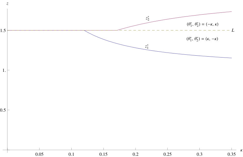 Figure 1
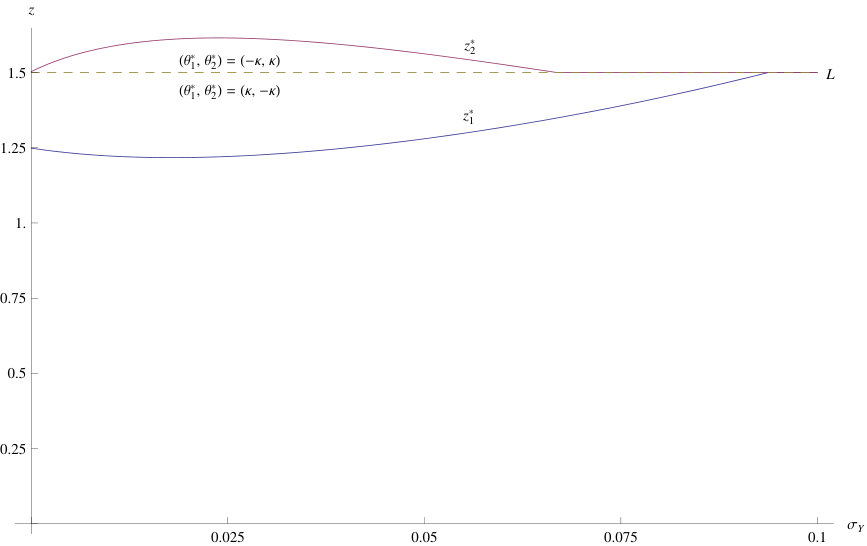 Figure 2
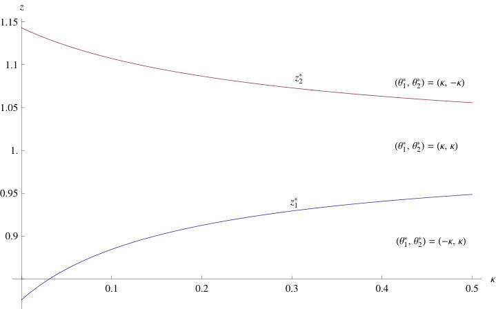 Figure 3
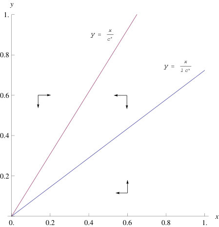 Figure 4
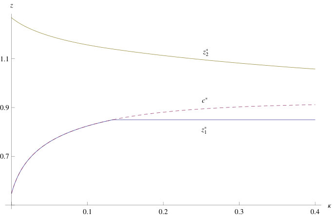 Figure 5
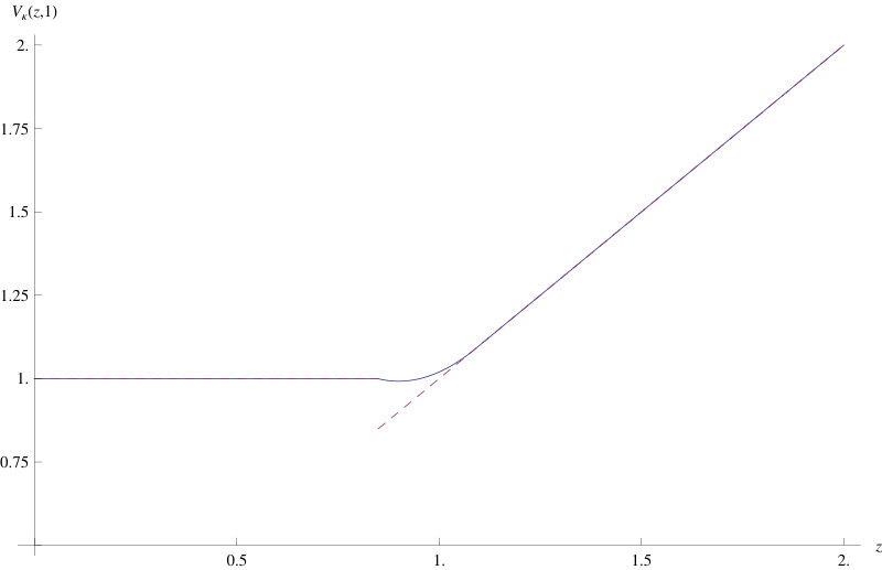 Figure 6
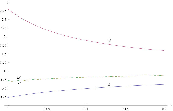 Figure 7
Peer Reviews
No public reviews on file for this paper yet. If you reviewed it on a platform where reviews are public (OpenReview, ICLR, NeurIPS, ICML), you can paste yours below so the community can read it here.
Videos
No videos yet. Explain this paper in a talk, walkthrough, or lecture? Add one.
Taxonomy
TopicsCapital Investment and Risk Analysis · Climate Change Policy and Economics · Economic theories and models
A Solvable Two-dimensional Optimal Stopping Problem in the Presence of Ambiguity
Luis H. R. Alvarez E. Sören Christensen Department of Accounting and Finance, Turku School of Economics, FIN-20014 University of Turku, Finland, E-mail: [email protected] Seminar, Christian-Albrechts-Universität zu Kiel, Ludewig-Meyn-Str. 4, D-24098 Kiel, Germany, E-mail: [email protected]
Abstract
According to conventional wisdom, ambiguity accelerates optimal timing by decreasing the value of waiting in comparison with the unambiguous benchmark case. We study this mechanism in a multidimensional setting and show that in a multifactor model ambiguity does not only influence the rate at which the underlying processes are expected to grow, it also affects the rate at which the problem is discounted. This mechanism where nature also selects the rate at which the problem is discounted cannot appear in a one-dimensional setting and as such we identify an indirect way of how ambiguity affects optimal timing.
AMS Subject Classification: 60J60, 60G40, 62L15, 91G80
Keywords: -ambiguity, geometric Brownian motion, optimal stopping, worst case prior.
1 Introduction
Ambiguity is known to accelerate the rational exercise of timing decisions in comparison with the unambiguous benchmark model. The main reason for this finding is that higher ambiguity decreases the value associated with the worst case scenario while leaving the exercise payoff unchanged. Since waiting is, however, optimal as long as the value of waiting dominates the exercise payoff, ambiguity tends to shrink the continuation set where waiting is optimal and, consequently, speeds up optimal timing. Since ambiguity interplays with the volatility of the underlying stochastic factor dynamics it is clear that its impact on the timing decision is more involved and not necessarily symmetric in a multidimensional setting. Our objective is to investigate this question in a class of solvable two-dimensional stopping problems.
The literature investigating ambiguity and its impact on decision making is extensive. Within an atemporal multiple priors setting the theory originates from the path breaking study Gilboa and Schmeidler, (1989) (see also Bewley, (2002), Klibanoff et al., (2005), Maccheroni et al., (2006) and Nishimura and Ozaki, (2006)). The axiomatization based on atemproal analysis was subsequently extended into an intertemporal recursive multiple priors setting by, among others, Epstein and Wang, (1994), Chen and Epstein, (2002), Epstein and Miao, (2003), and Epstein and Schneider, (2003). The impact of ambiguity on optimal timing decisions was first investigated by Nishimura and Ozaki, (2004) in a job search model. The analysis of ambiguity on optimal timing decisions have subsequently been extended to various directions. Nishimura and Ozaki, (2007) considered the impact of Knightian uncertainty on the optimal investment timing decisions in a continuous time model based on geometric Brownian motion. Alvarez E., (2007) investigated the impact of Knightian uncertainty on monotone one-sided stopping problems and expressed the value as well as the optimality conditions for the stopping boundaries in terms of the monotone fundamental solutions characterizing the Green-function of the underlying diffusion process. Riedel, (2009) developed within a discrete time setting a general minmax martingale approach to optimal stopping problems in the presence of ambiguity aversion. Cheng and Riedel, (2013), in turn, extended the analysis developed in Riedel, (2009) to a continuous time setting and identified the value as the smallest right continuous -martingale dominating the payoff process. Miao and Wang, (2011) considered the impact of ambiguity on timing in a model based on a general discrete time Feller-continuous Markov process. Christensen, (2013) investigates optimal stopping of linear diffusions in the presence of Knightian uncertainty and identifies explicitly the minimal excessive mappings generating the worst case measure and states a general characterization for the value and optimal timing policy in terms of these mappings.
We consider the impact of ambiguity on optimal timing in a multidimensional setting by solving an optimal stopping problem in the case where the exercise payoff is positively homogeneous and the underlying diffusions are geometric Brownian motions. Since a positively homogeneous function is not necessarily continuous, our results cast simultaneously light on the optimal policy and its value also in discontinuous multidimensional cases. By utilizing the fact that the ratio of two geometric Brownian motions constitutes a geometric Brownian motion, we first reduce the dimensionality of the considered problem and express it in terms of an associated one-dimensional problem which can be analyzed by relying on the approach based on minimal excessive functions developed in Christensen, (2013). Even though the transformed problem is one-dimensional, it differs in two significant ways from standard one dimensional timing problems in the presence of ambiguity. First of all, in the transformed problem ambiguity does not only affect the rate at which the value is expected to grow, it also affects the rate at which the exercise payoff is discounted. This mechanism where nature also selects the rate at which the problem is discounted cannot appear in an ordinary one-dimensional setting. Therefore, our results present a new indirect way of how ambiguity affects optimal timing. Second, since the optimal timing decision is affected by two random factors the density generators characterizing the worst case measure may separately switch from one extreme to another at different interconnected states. This is again a result which cannot arise in a single factor setting.
The contents of this study are as follows. In section 2 we describe the underlying stochastic dynamics and state the considered problem. Our main findings are then summarized in section 3. Our general findings are illustrated in various explicit examples in section 4. Section 5 then concludes our study.
2 Underlying Dynamics and Problem Setting
Let be an ordinary two-dimensional Brownian motion under the measure and assume that the underlying processes follow under the measure the stochastic dynamics characterized by the stochastic differential equations
[TABLE]
where and are known constants.
As usually in models subject to Knightian uncertainty, let the degree of ambiguity be given and denote by the set of all probability measures, that are equivalent to with density process of the form
[TABLE]
for a progressively measurable process with for all and . Under the measure defined by the likelihood ratio
[TABLE]
we naturally have that
[TABLE]
is an ordinary 2-dimensional -Brownian motion. Thus, we notice that under a measure the dynamics of the underlying processes read as
[TABLE]
where denotes a two-dimensional -Brownian motion.
Given the underlying processes and the class of equivalent measures generated by the density process , we now plan to investigate the following optimal stopping problem
[TABLE]
where is a known non-negative and measurable function which is assumed to be positively homogeneous of degree one in the following unless otherwise stated. For the sake of comparison, denote the value of the optimal timing policy in the absence of ambiguity by (cf. Alvarez E. and Virtanen, (2005) and Christensen and Irle, (2011))
[TABLE]
Before stating our main results on the optimal timing policy and its value we first establish the following result characterizing the impact of ambiguity on the optimal stopping strategy and its value in a general setting.
Lemma 2.1**.**
Ambiguity decreases the value of the optimal stopping policy and accelerates optimal timing by shrinking the continuation region where waiting is optimal. More precisely, for a general measurable and non-negative reward function it holds that for all and , where and .
Proof.
Inequality follows directly from the definition of the value of the optimal stopping policy in the presence of ambiguity. Denote the continuation regions associated to the considered stopping problems by and . It is clear that if then implying that as well and, consequently, that . ∎
Lemma 2.1 demonstrates that ambiguity accelerates optimal exercise by shrinking the continuation set at which waiting is optimal. As intuitively is clear higher ambiguity also decreases the value of the optimal policy. It is worth emphasizing that the negativity of the impact of ambiguity on the value and the incentives to wait is more generally valid than just within the considered class of problems, since the proof can be directly extended to a higher-dimensional setting where the underlying processes are more general than just geometric Brownian motions.
3 Optimal Timing Policy
Our objective is now to develop our main results on the considered class of optimal stopping problems. We can now make the following useful observation summarizing a set of conditions under which the worst case prior can be straightforwardly identified and, consequently, under which both the value as well as the optimal stopping policy can be determined from a standard stopping problem.
Lemma 3.1**.**
*For a general measurable and non-negative reward function the following holds true:
(A) Assume that is monotonically increasing as a function of and monotonically decreasing as a function of . Then the worst case measure is generated by the choice .
(B) Assume that is monotonically increasing as a function of and . Then the worst case measure is generated by the choice .
(C) Assume that is monotonically decreasing as a function of and monotonically increasing as a function of . Then the worst case measure is generated by the choice .
(D) Assume that is monotonically decreasing as a function of and . Then the worst case measure is generated by the choice .
In all cases stated above we have*
[TABLE]
Proof.
We only prove part (A), since proving the rest of the claims is completely analogous. It is now clear by definition of the value that
[TABLE]
In order to reverse this inequality, we notice that since
[TABLE]
the alleged claim follows directly from standard comparison results after invoking the a.s.-bounds
[TABLE]
the strong uniqueness of the solutions, and the assumed monotonicity of the exercise payoff. ∎
Lemma 3.1 characterizes the worst case measures in the case where the reward function is strictly monotonic as a function of the underlying state variables. This simplifies the analysis since it delineates circumstances under which the worst case measure can be determined solely based on the monotonicity properties of the reward without having to solve simultaneously the worst case density generators and the value of the optimal policy. Since the measure is in the cases treated in Lemma 3.1 independent of the prevailing state, we notice that under the conditions of Lemma 3.1 the value of the optimal policy preserves the homogeneity of the exercise payoff (cf. Olsen and Stensland, (1992) for a general treatment in the absence of ambiguity; see also McDonald and Siegel, (1986) and Hu and Øksendal, (1998)).
Having stated the cases associated with the monotone cases, we now plan to proceed into the analysis of the more general cases resulting into endogenous state dependent switching of the density generators determining the worst case measure. In order to characterize the worst case measure in the considered class of problems, let us first consider the determination of the optimal density generators by relying on standard dynamic programming arguments. To this end, we denote by
[TABLE]
the differential operator associated with the underlying processes under the measure and assume now that the function is twice continuously differentiable on . A standard application of the Itô-Döblin theorem then yields
[TABLE]
It is then clear from this expression that the density generators associated with the worst case scenario are of the form and Thus, if the function is chosen so that it satisfies the partial differential equation on some open subset with compact closure in , then we have
[TABLE]
for all admissible density generators , , and . Noticing that and for all admissible and then shows that
[TABLE]
with equality only when . Even though this observation is interesting as a characterization for the optimal policy and its value, it has at least two weaknesses from the perspective of the considered class of problems. First of all, it is not beforehand clear whether the value of the optimal policy is actually smooth enough for the utilization of the Itô-Döblin theorem. Fortunately, there are extensions which do not require as much smoothness (see, for example, pp. 315 – 318 in Øksendal, (2003) or Section IV.7 in Protter, (2005)) which could be utilized in the determination of the value and worst case measure. Second, the characterization of the value on the continuation region as a solution of a partial differential equation overlooks the homogeneity properties of the considered class of problems and, therefore, does not make use of the possibility to reduce the dimensionality of the considered problem by focusing on the ratio process instead of the two-dimensional process .
Given the observations above, let us now follow the approach originally developed in Christensen, (2013) and investigate if we can identify a set of minimal harmonic functions which can be utilized in the determination of the value of an optimal timing policy. We also refer to Beibel and Lerche, (1997) (see also Lerche and Urusov, (2007), Christensen and Irle, (2011), and Gapeev and Lerche, (2011)) for related considerations for usual optimal stopping problems.
Put formally, our objective is to identify a twice continuously differentiable function such that , where . In order to achieve this we plan to utilize the positive homogeneity of the exercise payoff and investigate if it is possible to find homogeneous solutions for the partial differential equation characterizing the value on the continuation region. In the present setting
[TABLE]
indicating that the density generators resulting into a worst case measure are now and . Consequently, if then we necessarily have
[TABLE]
for ,
[TABLE]
for , and
[TABLE]
for . Moreover, for , for , and for .
In order to determine the harmonic mappings needed for the determination of the value and its optimal policy, we first notice that if condition is satisfied then the quadratic equation
[TABLE]
has two roots
[TABLE]
In that case we can define the monotonically decreasing, twice continuously differentiable, and strictly convex function On the other hand, condition also guarantees that the quadratic equation
[TABLE]
has two roots
[TABLE]
In this case we can define the monotonically increasing and twice continuously differentiable function when and when . Notice that condition implies that guaranteeing that is strictly convex in that case. Finally, in order to capture the potential cases appearing in multiple boundary problems, we again assume that condition is satisfied and define the twice continuously differentiable function as
[TABLE]
when . If, however, then
[TABLE]
where
[TABLE]
Since
[TABLE]
we notice that is again twice continuously differentiable on , monotonically decreasing on , and monotonically increasing on . Moreover, condition guarantees that is strictly convex on as well, and satisfies the condition on . It is worth noticing that if , then the function admits the representation , where
[TABLE]
Note that since as the function reduces to when .
Having characterized the key harmonic functions needed in the characterization of the value of the optimal timing policy, we now investigate the behavior of the ratio
[TABLE]
for all and . A set of auxiliary results characterizing the key role of the harmonic functions in the determination of the worst case measure as well as the value of the optimal policy is now summarized in the following (see Lemma 1 in Christensen, (2013)).
Lemma 3.2**.**
Assume that and denote by the measure induced by the density generators , where . Then,
[TABLE]
and
[TABLE]
where is a 2-dimensional Brownian motion under the measure . Moreover, for any stopping time , admissible density generator , and we have
[TABLE]
Proof.
We first observe that under our assumptions is strictly convex and twice continuously differentiable on . Consequently, the standard Itô-Döblin theorem applies. Given this observation and utilizing the identity (3.2) in the homogeneous case yields
[TABLE]
where . Assume that is an open subset with compact closure in and let denote the first exit time of the process from . The smoothness of the function and behavior of the ratio process (it can be sandwiched between two geometric Brownian motions) then guarantees that all the functional forms are bounded on open subsets with compact closure on . Since and for all and admissible density generators we notice that
[TABLE]
demonstrating that the stopped process is a bounded positive -submartingale. For we have
[TABLE]
proving that the process is a bounded positive local -martingale. Analogous computations demonstrate that the process is actually a positive -martingale and, therefore, a supermartingale. Finally, it is clear that under the measure the underlying processes as well as their ratio evolve according to the random dynamics characterized by the stochastic differential equations (3.7), (3.8), and (3.9). ∎
Lemma 3.2 essentially shows how the function induces an appropriate class of worst case supermartingales for the considered class of processes. A first result of this type is given in the next proposition.
Proposition 3.3**.**
If
[TABLE]
then .
Proof.
Assume that the set and let It is then clear that (see part (i) of Theorem 3 in Christensen, (2013))
[TABLE]
for all , , and . Hence, we have found that . Since for all we notice that
[TABLE]
proving that as claimed.
∎
Interestingly, the ratio process (3.9) is an ordinary linear diffusion with known infinitesimal characteristics which helps us in the determination of the expected first exit times from bounded open intervals in . This is formally summarized in our next lemma.
Lemma 3.4**.**
Assume that so that . For all we have
[TABLE]
where
[TABLE]
,
[TABLE]
* , , , and .*
Proof.
constitutes the density of the scale function and the density of the speed measure of the diffusion characterized by (3.9). The result then follows from the analysis in, for example, Chapter 4 in Itô and McKean, (1974). ∎
Lemma 3.4 essentially guarantees that the first exit times of from bounded open intervals in is -a.s. finite. This observation as well as the properties of the function plays a central role in the characterization of the optimal timing policy and its value as summarized in our next theorem.
Theorem 3.5** (Two-sided case).**
Assume that there are two points , , for some such that . Then
- (A)
V_{\kappa}(x,y)=\Pi_{c^{\ast}}(z_{i}^{\ast})yh_{c^{\ast}}(x/y)\mbox{ for all (x,y)\in\mathbb{R}_{+}^{2}with }x/y\in(z_{1}^{\ast},z_{2}^{\ast})\mbox{ andi=1,2}.* *
- (B)
If for all , then
[TABLE]
- (C)
Let be such that -a.s. for all initial points with . Then, is an equilibrium in the sense that for all initial points with it holds that
[TABLE]
Proof.
First note that the process
[TABLE]
is a positive -martingale by Lemma 3.2. Using this, it holds that for all and all initial points with
[TABLE]
It furthermore holds that as given in (C) is -a.s. finite by Lemma 3.4 for all initial points with and hence . Moreover, by optional sampling,
[TABLE]
This yields that for both inequalities in the calculations above are indeed equations, i.e.
[TABLE]
Since we notice that
[TABLE]
implying that for all , i.e., the first inequality in (A). The calculations furthermore prove the second equilibrium condition in (C).
To prove the opposite inequality in (A) and the first equilibrium condition in (C) we obtain – using again that the admissible stopping policy is -a.s. finite and on the set as well as Lemma 3.2 –
[TABLE]
for all , proving (A). Now, (A) together with the last inequalities im Lemma 3.2, yields the first part of (C).
Finally, noticing that for all we have
[TABLE]
showing that , viz. (B). ∎
According to Proposition 3.3 the points belonging to the set are part of the stopping set where waiting is suboptimal independently of the reference point . This is an interesting finding since it provides a straightforward technique for identifying elements in the stopping region. Theorem 3.5 delineates a set of conditions under which the optimal stopping strategy constitutes a two boundary policy and the value can be expressed in terms of the function .
As in the case of a general reference point we again notice that the functions and can be utilized in the analysis of the optimal timing policy and the associated worst case measure for the one-sided boundary situation. This is summarized in the following two theorems.
Theorem 3.6** (lower-boundary case).**
Assume that condition is met and that there exists a point . Then
- (A)
* whenever . *
- (B)
If for all , then
[TABLE]
- (C)
Let be such that -a.s. for all initial points with . Then, is an equilibrium in the sense that for all initial points with it holds that
[TABLE]
Proof.
Noticing that condition yields that is -a.s. finite is met for all initial points with , the statement holds by a straightforward modification of the arguments in the proof of Theorem 3.5. ∎
Not surprisingly, we obtain analogously
Theorem 3.7** (upper-boundary case).**
Assume that condition is met and that there exists a point . Then
- (A)
* whenever . *
- (B)
If for all , then
[TABLE]
- (C)
Let be such that -a.s. for all initial points with . Then, is an equilibrium in the sense that for all initial points with it holds that
[TABLE]
Remark 3.8. Proposition 3.3 together with the previous three theorems leads to a procedure for solving general versions of our stopping problem (2.5) as follows:
Determine the maximum points of the real functions for all to find
[TABLE] 2. 2.
The complement of forms a partition of into subcones. For each such cone , , find a parameter such that Theorem 3.5, 3.6, or 3.7 is applicable. Then, is a worst case prior for the corresponding subcone, defines the value function on it, and the first entrance time into is a (global) optimal stopping time for (2.5). For last claim, note that the underlying processes do not have jumps and therefore, the different connected components of the complement of do not communicate with each other.
The question arises whether this procedure can always be applied. In other words: Is one of the Theorem 3.5, 3.6, or 3.7 always applicable in Step 2? – The answer is yes under some mild assumptions. To see that this is indeed the case, assume that condition holds and consider, for fixed , , the functions and as functions of . It is clear that
[TABLE]
Since, for example,
[TABLE]
we observe now by utilizing the fact that the pointwise infimum of an affine function is concave and, thus, continuous, that is continuous as a function of . Since the maximum of continuous functions is continuous, we notice that is continuous as a function of too. The same argument is naturally valid for as well. Consequently, the difference
[TABLE]
is continuous as a function of . Now, there are three possible cases:
. Then there exists such that Theorem 3.6 is applicable whenever is a maximum (which is the case under standard continuity- and growths-assumptions on the reward function ). 2. 2.
. Then, whenever is a maximum, there exists such that Theorem 3.7 is applicable. 3. 3.
By continuity, there exists such that . Assuming again that the suprema are maxima, there exist two points such that Theorem 3.5 is applicable.
It is at this point worth emphasizing that our findings indicate that the representation of the value as the smallest element of an appropriately chosen function space developed in Christensen, (2013) applies in some cases in the present setting as well. In that case we have
[TABLE]
for all .
It is clear from the description above that the minimal harmonic functions in the present case differ from the ones appearing in the one-dimensional setting. There are two main reasons for this. First, the presence of two driving random factor dynamics implies that the underlying density generators may separately switch from one extreme to another at different states as is clear from the form of the sets and . Second, the assumed homogeneity of the exercise payoff implies that both the growth rate as well as the density generator associated with the numeraire variable affect the rate at which the problem is discounted. This mechanism where nature also selects the rate at which the problem is discounted cannot naturally appear in a one-dimensional setting where discounting is not affected by the characteristics of the underlying factor dynamics.
4 Explicit Illustrations
4.1 Compound Option
In order to illustrate an option where the stopping region constitutes a closed interval on we now consider the compound option case
[TABLE]
where the strike prices satisfy the inequality . We also assume that guaranteeing that and . Since on we notice by solving the optimization problem
[TABLE]
that the lower optimal exercise boundary is
[TABLE]
Analogously, since on we notice by solving the optimization problem
[TABLE]
that the upper optimal exercise boundary is
[TABLE]
Utilizing Proposition 3.3 shows that is a subset of the optimal stopping set. Therefore, the value reads as , where
[TABLE]
Moreover, the optimal density generators now read as
[TABLE]
It is at this point worth emphasizing that the impact of ambiguity on the optimal timing policy is asymmetric despite its seemingly simple symmetric structure. To see that this is indeed the case, we first observe that under our assumptions and . Given these sensitivities, we now investigate when a corner solution may arise. To this end we first observe that whenever and whenever . Since , , , and , we notice that if a corner solution is attained in the unambiguous benchmark setting, that is, if and , then there exists two critical degrees so that for and for . We also notice that the optimal timing rules approach the Marshallian investment rule in the limit as . More precisely, and . The boundaries are illustrated as functions of the degree of ambiguity in Figure 1 under the parameter assumptions and (implying that and ).
The impact of increased volatility on the optimal exercise boundaries depends on the exact parametrization of the problem and, therefore, on the degree of ambiguity. To see that this is indeed the case, we first notice that
[TABLE]
Since
[TABLE]
whenever , we notice that the impact of higher volatility on the optimal exercise thresholds is ambiguous. This is explicitly illustrated in Figure 2 under the parameter assumptions and . As is clear from this figure, the impact of increased volatility on optimal timing is not necessarily decelerating in the presence of ambiguity.
4.2 Floor Option
In order to illustrate a case where the determination of the worst case measure involves the determination of the switching point at which the drift of the underlying is taken from one extreme to another let us consider the reward (cf. Guo and Shepp, (2001)). Assume that . In line with our general results we now analyze the ratio
[TABLE]
where is defined in (3.6). It is now a straightforward exercise in ordinary differentiation to show that a local maximum is attained on the set at
[TABLE]
Plugging this into the ratio yields
[TABLE]
On the other hand, since is monotonically decreasing on the ratio is increasing on . Consequently, the lower optimal boundary is attained at . Therefore, we have
[TABLE]
yielding
[TABLE]
and
[TABLE]
In this case, the value of the optimal policy reads
[TABLE]
From this expression we notice that the stopping region now reads as . Moreover, we clearly have , , and .
It is at this point worth emphasizing that the worst case measure is characterized by the density generators
[TABLE]
Interestingly, the worst case measure is such that it pushes on the underlying process upwards towards the set where the drift once again switches pushing the process back towards the set . Analogously, the worst case measure pushes on the underlying process towards the set where the drift once again switches and pushes back towards the set .
The optimal exercise boundaries are illustrated in Figure 3 as functions of the degree of ambiguity under the assumptions that and .
4.3 Straddle Option
In order to illustrate a nontrivial two-boundary case where the threshold where the density generators switch from one extreme to another does not coincide with one of the optimal boundaries, we now consider the straddle option under the assumption . It is clear that in this case the candidate boundaries have to be determined from the first order optimality conditions
[TABLE]
Utilizing now the strict convexity, smoothness, and limiting behavior of the function shows that for all optimality condition (4.1) has a unique root and that is increasing as a function of . Analogously, we also notice that for all optimality condition (4.1) has a unique root and that is increasing as a function of . It is also clear that
[TABLE]
Combining these observations with the limiting behavior of shows that , , , and . Consequently, there is at least one so that . Combining this observation with the monotonicity of and as a function of then prove that is unique and that constitute the optimal stopping boundaries satisfying the inequality . We notice that in the present example the value of the optimal policy reads
[TABLE]
From this expression we notice that the stopping region again reads as .
These quantities are illustrated as functions of the degree of ambiguity in Figure 4 under the assumptions that , and .
It is at this point worth noticing that in the present example the optimal density generators read as
[TABLE]
Thus, in contrast with the floor option case, the states at which the density generators switch form one extreme state to another do not coincide with the exercise thresholds. An illustration can be found in Figure 5.
4.4 Digital Option
In order to illustrate our findings in a discontinuous framework, we now focus on a digital option with an exercise payoff
[TABLE]
where is a known constant. Note that we rule out the case since that coincides with the floor option case treated earlier. Since , we notice that in this case we have to focus on the ratio
[TABLE]
Standard analysis yields that if condition holds, then
[TABLE]
and
[TABLE]
Noticing now that for all , , and
[TABLE]
demonstrates that equation has at least one root . The monotonicity of as a function of implies that is unique. Moreover, we notice that and
[TABLE]
In light of our results on the floor option, we notice immediately that and
[TABLE]
as long as inequality holds. If, however, , then and the optimal constitutes the unique root of equation
[TABLE]
on the set . Interestingly, despite the discontinuity of exercise payoff, we find that the value reads in this case as
[TABLE]
The stopping region has a similar structure with the one arising in the two previous examples.
The value is illustrated in Figure 6 under the assumptions , and (implying that and ).
The optimal boundaries are, in turn, illustrated in Figure 7 as functions of the degree of ambiguity under the assumptions , and .
5 Conclusions
We analyzed the impact of ambiguity on optimal stopping in the case where the exercise payoff is positively homogeneous and the underlying diffusions are two geometric Brownian motions. Utilizing the fact that the ratio of two geometric Brownian motions constitutes a geometric Brownian motion we reduced the dimensionality of the problem and extended the approach based on minimal excessive functions developed in Christensen, (2013) to the considered setting. Since a positively homogeneous function is not necessarily continuous, our results cast light on the optimal policy and its value also in nonsmooth cases.
There are several interesting directions towards which our analysis could naturally be extended. First, even though geometric Brownian motion constitutes the key benchmark process in financial and economic applications of optimal stopping, it would be of interest to study whether our principal conclusions would remain valid in a more general setting. The same argument is valid for the chosen payoff structure as well. Even though linearly homogeneous payoff structures play a prominent role in economic applications, analyzing the impact of more complex payoffs would be an interesting direction towards which our analysis could be extended. Both proposed extensions are mathematically extremely challenging and out of the scope of our current study.
The reference list from the paper itself. Each links out to its DOI / PubMed record.
- 1Alvarez E., (2007) Alvarez E., L. H. R. (2007). Knightian uncertainty, κ 𝜅 \kappa -ignorance, and optimal timing. Technical Report 25, Aboa Center of Economics, University of Turku.
- 2Alvarez E. and Virtanen, (2005) Alvarez E., L. H. R. and Virtanen, J. (2005). A certainty equivalent characterization of a class of perpetual american contingent claims. Discussion Paper Series 1/2005, Turku School of Economics and Business Administration.
- 3Beibel and Lerche, (1997) Beibel, M. and Lerche, H. R. (1997). A new look at optimal stopping problems related to mathematical finance. Statist. Sinica , 7(1):93–108. Empirical Bayes, sequential analysis and related topics in statistics and probability (New Brunswick, NJ, 1995).
- 4Bewley, (2002) Bewley, T. F. (2002). Knightian decision theory. I. Decis. Econ. Finance , 25(2):79–110.
- 5Chen and Epstein, (2002) Chen, Z. and Epstein, L. (2002). Ambiguity, risk, and asset returns in continuous time. Econometrica , 70(4):1403–1443.
- 6Cheng and Riedel, (2013) Cheng, X. and Riedel, F. (2013). Optimal stopping under ambiguity in continuous time. Math. Financ. Econ. , 7(1):29–68.
- 7Christensen, (2013) Christensen, S. (2013). Optimal decision under ambiguity for diffusion processes. Math. Methods Oper. Res. , 77(2):207–226.
- 8Christensen and Irle, (2011) Christensen, S. and Irle, A. (2011). A harmonic function technique for the optimal stopping of diffusions. Stochastics , 83(4-6):347–363.