TL;DR
This paper introduces new metrics, PAPE and AUPEC, for evaluating individualized treatment rules using experimental data, providing exact variance estimates without modeling assumptions, applicable to complex algorithms.
Contribution
It proposes novel evaluation metrics (PAPE and AUPEC) and their variance estimation methods for assessing ITRs, including when using the same data for estimation and evaluation.
Findings
PAPE and AUPEC effectively measure ITR performance.
Variance formulas enable precise evaluation without resampling.
Method applicable to complex machine learning-based ITRs.
Abstract
The increasing availability of individual-level data has led to numerous applications of individualized (or personalized) treatment rules (ITRs). Policy makers often wish to empirically evaluate ITRs and compare their relative performance before implementing them in a target population. We propose a new evaluation metric, the population average prescriptive effect (PAPE). The PAPE compares the performance of ITR with that of non-individualized treatment rule, which randomly treats the same proportion of units. Averaging the PAPE over a range of budget constraints yields our second evaluation metric, the area under the prescriptive effect curve (AUPEC). The AUPEC represents an overall performance measure for evaluation, like the area under the receiver and operating characteristic curve (AUROC) does for classification, and is a generalization of the QINI coefficient utilized in uplift…
Click any figure to enlarge with its caption.
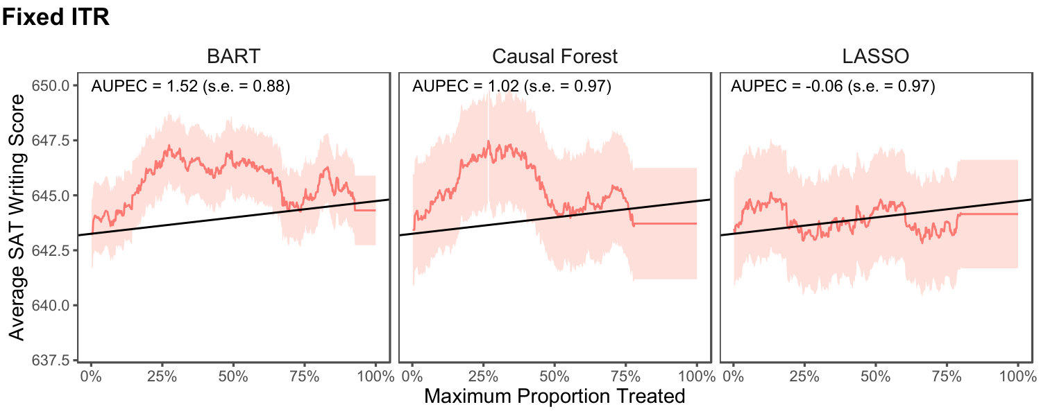 Figure 1
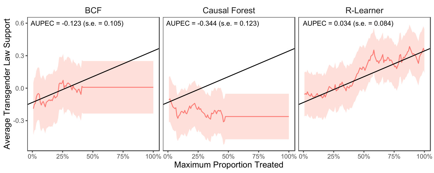 Figure 2
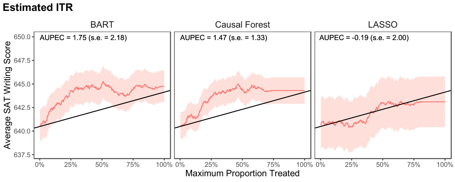 Figure 3
| Estimator | truth | coverage | bias | s.d. | coverage | bias | s.d. | coverage | bias | s.d. |
|---|---|---|---|---|---|---|---|---|---|---|
| Low treatment effect | ||||||||||
| High treatment effect | ||||||||||
| Estimator | truth | coverage | bias | s.d. | truth | coverage | bias | s.d. | truth | coverage | bias | s.d. |
|---|---|---|---|---|---|---|---|---|---|---|---|---|
| Low Effect | ||||||||||||
| High Effect | ||||||||||||
| BART | Causal Forest | LASSO | |||||||
| est. | s.e. | treated | est. | s.e. | treated | est. | s.e. | treated | |
| Fixed ITR | |||||||||
| No budget constraint | |||||||||
| Reading | 100% | 84.3% | 84.4% | ||||||
| Math | 86.7 | 80.3 | 78.7 | ||||||
| Writing | 92.7 | 78.0 | 80.0 | ||||||
| \hdashline Budget constraint | |||||||||
| Reading | 20 | 20 | 20 | ||||||
| Math | 20 | 20 | 20 | ||||||
| Writing | 20 | 20 | 20 | ||||||
| Estimated ITR | |||||||||
| No budget constraint | |||||||||
| Reading | 99.3% | 86.6% | 87.6% | ||||||
| Math | 84.7 | 79.1 | 75.2 | ||||||
| Writing | 88.0 | 67.4 | 74.8 | ||||||
| \hdashline Budget constraint | |||||||||
| Reading | 20 | 20 | 20 | ||||||
| Math | 20 | 20 | 20 | ||||||
| Writing | 20 | 20 | 20 | ||||||
| Causal Forest | BART | |||||
| vs. BART | vs. LASSO | vs. LASSO | ||||
| est. | CI | est. | CI | est. | CI | |
| Fixed ITR | ||||||
| Math | [0.35, 3.45] | [0.50, 4.16] | [2.39, 2.95] | |||
| Reading | [0.79, 4.51] | [1.49, 4.11] | [4.02, 2.92] | |||
| Writing | [1.66, 2.42] | [0.27, 5.65] | [0.53, 5.15] | |||
| Estimated ITR | ||||||
| Reading | [3.99, 1.69] | [1.05, 2.15] | [0.90, 4.30] | |||
| Math | [2.57, 3.43] | [1.32, 2.00] | [1.99, 3.53] | |||
| Writing | [1.63, 0.80] | [0.76, 3.98] | [1.32, 4.26] | |||
| Individual | |||||
|---|---|---|---|---|---|
| A | 1 | 1 | 2 | 0 | 2 |
| B | 1 | 0 | 3 | 1 | 3 |
| C | 0 | 0 | 1 | 1 | 1 |
| D | 0 | 1 | 1 | 1 | 0 |
| E | 1 | 0 | 3 | 0 | 3 |
| BCF | Causal Forest | R-Learner | |||||||
|---|---|---|---|---|---|---|---|---|---|
| est. | s.e. | treated | est. | s.e. | treated | est. | s.e. | treated | |
| No budget constraint | 48.4% | 47.5% | 100% | ||||||
| 20% Budget constraint | 20% | 20% | 20% | ||||||
Peer Reviews
No public reviews on file for this paper yet. If you reviewed it on a platform where reviews are public (OpenReview, ICLR, NeurIPS, ICML), you can paste yours below so the community can read it here.
Code & Models
Videos
No videos yet. Explain this paper in a talk, walkthrough, or lecture? Add one.
Experimental Evaluation of Individualized Treatment
Rules††thanks: We thank Naoki Egami, Colin Fogarty, Zhichao Jiang, Susan Murphy, Nicole Pashley, Stefan Wager, three anonymous reviewers, and especially the Associate Editor for many helpful comments. We thank Dr. Hsin-Hsiao Wang who inspired us to write this paper. Imai thanks the Alfred P. Sloan Foundation for partial support of this research. The proposed methodology is implemented through an open-source R package, evalITR, which is freely available for download at the Comprehensive R Archive Network (CRAN; https://CRAN.R-project.org/package=evalITR).
Kosuke Imai Michael Lingzhi Li Professor, Department of Government and Department of Statistics, Harvard University, Cambridge, MA 02138. Phone: 617–384–6778, Email: [email protected], URL: https://imai.fas.harvard.eduOperation Research Center, Massachusetts Institute of Technology, Cambridge, MA 02139. [email protected]
(First version: May 15, 2019
This version: )
Abstract
The increasing availability of individual-level data has led to numerous applications of individualized (or personalized) treatment rules (ITRs). Policy makers often wish to empirically evaluate ITRs and compare their relative performance before implementing them in a target population. We propose a new evaluation metric, the population average prescriptive effect (PAPE). The PAPE compares the performance of ITR with that of non-individualized treatment rule, which randomly treats the same proportion of units. Averaging the PAPE over a range of budget constraints yields our second evaluation metric, the area under the prescriptive effect curve (AUPEC). The AUPEC represents an overall performance measure for evaluation, like the area under the receiver and operating characteristic curve (AUROC) does for classification, and is a generalization of the QINI coefficient utilized in uplift modeling. We use Neyman’s repeated sampling framework to estimate the PAPE and AUPEC and derive their exact finite-sample variances based on random sampling of units and random assignment of treatment. We extend our methodology to a common setting, in which the same experimental data is used to both estimate and evaluate ITRs. In this case, our variance calculation incorporates the additional uncertainty due to random splits of data used for cross-validation. The proposed evaluation metrics can be estimated without requiring modeling assumptions, asymptotic approximation, or resampling methods. As a result, it is applicable to any ITR including those based on complex machine learning algorithms. The open-source software package is available for implementing the proposed methodology.
Key Words: causal inference, heterogenous treatment effects, machine learning, precision medicine, uplift modeling
1 Introduction
In today’s data-rich society, the individualized (or personalized) treatment rules (ITRs), which assign different treatments to individuals based on their observed characteristics, play an essential role. Examples include personalized medicine and micro-targeting in business and political campaigns (e.g., Hamburg and Collins, 2010; Imai and Strauss, 2011). In the causal inference literature, a number of researchers have developed methods to estimate optimal ITRs using a variety of machine learning algorithms (see e.g., Qian and Murphy, 2011; Zhang et al., 2012; Fu et al., 2016; Luedtke and van der Laan, 2016a, b; Zhou et al., 2017; Athey and Wager, 2018; Kitagawa and Tetenov, 2018). In addition, applied researchers often use machine learning algorithms to estimate heterogeneous treatment effects and then construct ITRs based on the resulting estimates.
In this paper, we consider a common setting, in which a policy-maker wishes to experimentally evaluate the empirical performance of an ITR before implementing it in a target population. Such evaluation is also essential for comparing the efficacy of alternative ITRs. Specifically, we show how to use a randomized experiment for evaluating ITRs. We propose two new evaluation metrics. The first is the population average prescriptive effect (PAPE), which compares an ITR with a non-individualized treatment rule that randomly assigns the same proportion of units to the treatment condition. The PAPE represents the difference between the average outcome under the ITR and that under the random treatment rule. The key idea is that a well-performing ITR should outperform the random treatment rule, which does not utilize any individual-level information.
Averaging the PAPE over a range of budget constraints yields our second evaluation metric, the area under the prescriptive effect curve (AUPEC). Like the area under the receiver and operating characteristic curve (AUROC) for classification, the AUPEC represents an overall summary measure of how well an ITR performs over the random treatment rule that treats the same proportion of units.
We estimate these evaluation metrics using Neyman (1923)’s repeated sampling framework (see Imbens and Rubin, 2015, Chapter 6). An advantage of this approach is that it does not require any modeling assumption or asymptotic approximation. As a result, we can evaluate a broad class of ITRs including those based on complex machine learning algorithms. We show how to estimate the PAPE and AUPEC with a minimal amount of finite sample bias and derive the exact variance solely based on random sampling of units and random assignment of treatment.
We further extend this methodology to a common evaluation setting, in which the same experimental data is used to both estimate and evaluate ITRs. In this case, our finite-sample variance calculation is exact and directly incorporates the additional uncertainty due to random splits of data used for cross-validation. We implement the proposed methodology through an open-source R package.
Our simulation study demonstrates the accurate coverage of the proposed confidence intervals in small samples (Section 5). We also apply our methods to the Project STAR (Student-Teacher Achievement Ratio) experiment and compare the empirical performance of ITRs based on several popular methods (Section 6). Our evaluation approach addresses theoretical and practical difficulties of conducting reliable statistical inference for ITRs.
Relevant Literature.
A large number of existing studies have focused on the derivation of optimal ITRs that maximize the population average value. For example, Qian and Murphy (2011) use penalized least squares whereas Zhao et al. (2012) show how a support vector machine can be used to derive an optimal ITR. Another popular approach is based on doubly-robust estimation (e.g., Dudík et al., 2011; Zhang et al., 2012; Chakraborty et al., 2014; Jiang and Li, 2016; Athey and Wager, 2018; Kallus, 2018).
We propose a general methodology for empirically evaluating and comparing the performance of various ITRs including the ones proposed by these and other authors. While many of these methods come with uncertainty measures, even those that produce standard errors rely on asymptotic approximation, modeling assumptions, or resampling methods. In contrast, our methodology utilizes Neyman’s repeated sampling framework and does not require any of these assumptions or approximations.
There also exists a related literature on policy evaluation. Starting with Manski (2004), many studies focus on the derivation of regret bounds given a class of ITRs. For example, Kitagawa and Tetenov (2018) show that an ITR, which maximizes the empirical average value, is minimax optimal without a strong restriction on the class of ITRs, whereas Athey and Wager (2018) establish a regret bound for an ITR based on doubly-robust estimation in observational studies (see also Zhou et al., 2018). In addition, Luedtke and van der Laan (2016a, b) propose consistent estimators of the optimal average value even when an optimal ITR is not unique (see also Rai, 2018).
Our goal is different from these studies. We focus on statistical inference using the Neyman’s repeated sampling framework for the experimental evaluation of arbitrary ITRs including optimal or non-optimal and simple or complex ones. Our evaluation metric is also different from the existing metrics. In particular, to the best of our knowledge, we are the first to formally study the AUPEC as an AUROC-like summary measure for evaluation.
In contrast, much of the policy evaluation literature focus on the optimal average value, which is required to compute the regret of an ITR. Athey and Wager (2018) briefly discusses a quantity related to the PAPE in their empirical application, but this quantity evaluates an ITR against the treatment rule that randomly treats exactly one half of units rather than the same proportion as the one treated under the ITR. Although empirical studies in the campaign and marketing literatures have used “uplift modeling,” which is based on the PAPE (e.g., Imai and Strauss, 2011; Rzepakowski and Jaroszewicz, 2012; Gutierrez and Gérardy, 2016; Ascarza, 2018; Fifield, 2018), none develops formal estimation and inferential methods. We show that the AUPEC is a generalization of the QINI coefficient, which is a widely utilized statistic in uplift modeling (Radcliffe, 2007; Diemert et al., 2018). Thus, our theoretical results for the AUPEC apply directly to the QINI coefficient as well.
Another related literature is concerned with the estimation of heterogeneous effects. Researchers have explored the use of tree-based methods (e.g., Imai and Strauss, 2011; Athey and Imbens, 2016; Wager and Athey, 2018; Hahn et al., 2020), regularized regressions (e.g., Imai and Ratkovic, 2013; Künzel et al., 2018), and ensamble methods (e.g., van der Laan and Rose, 2011; Grimmer et al., 2017). In practice, the estimated heterogeneous treatment effects based on these machine learning algorithms are used to construct ITRs.
However, as Chernozhukov et al. (2019) point out, most machine learning algorithms, which require data-driven tuning parameters, cannot be regarded as consistent estimators of the conditional average treatment effect (CATE) unless strong assumptions are imposed. They propose a methodology to estimate heterogeneous treatment effects without such assumptions. Similar to theirs, our methodology does not depend on any modeling assumption and accounts for the uncertainty due to splitting of data. The key difference is that we focus on the evaluation of ITRs. In addition, our variance calculation is based on randomization and does not rely on asymptotic approximation.
Finally, Andrews et al. (2020) develops a conditional inference procedure, based on normal approximation, for the average value of the best-performing policy based on experimental or observational data. In contrast, we develop an unconditional exact inference for the difference in the average value between any pair of policies under a budget constraint. We also consider the evaluation of estimated policies based on the same experimental data using cross-validation whereas Andrews et al. focus on the evaluation of fixed policies.
2 Evaluation Metrics
In this section, we introduce our evaluation metrics. We first propose the population average prescriptive effect (PAPE) that, unlike the population average value, adjusts for the proportion of units treated by an ITR. The idea is that an efficacious ITR should outperform a non-individualized treatment rule, which randomly assigns the same proportion of units to the treatment condition. We extend the PAPE to the settings with a binding budget constraint. Finally, we propose the area under the prescriptive effect curve (AUPEC) as a univariate summary performance measure of an ITR under a range of budget constraint.
2.1 The Setup
Following the literature, we define an ITR as a deterministic map from the covariate space to the binary treatment assignment (e.g., Qian and Murphy, 2011; Zhao et al., 2012),
[TABLE]
Let denote the treatment assignment indicator variable, which is equal to if unit is assigned to the treatment condition, i.e., . For each unit, we observe the outcome variable as well as the vector of pre-treatment covariates, , where is the support of the outcome variable. We assume no interference between units and denote the potential outcome for unit under the treatment condition as for . Then, the observed outcome is given by .
Assumption 1 (No Interference between Units)
The potential outcomes for unit do not depend on the treatment status of other units. That is, for all , we have,
Under this assumption, the existing literature almost exclusively focuses on the derivation of an optimal ITR that maximizes the following population average value (e.g., Qian and Murphy, 2011; Zhao et al., 2012; Zhou et al., 2017),
[TABLE]
Next, we show that may not be the best evaluation metric in some cases.
2.2 The Population Average Prescriptive Effect
We now introduce our main evaluation metric, the Population Average Prescriptive Effect (PAPE). The PAPE is based on two ideas. First, it is reasonable to expect a good ITR to outperform a non-individualized treatment rule, which does not use any information about individual units when deciding who should receive the treatment. Second, a budget constraint should be considered since the treatment is often costly. This means that a good ITR should identify units who benefit from the treatment most. These two considerations lead to the random treatment rule, which assigns, with equal probability, the same proportion of units to the treatment condition, as a natural baseline for comparison.
Figure 1 illustrates the importance of accounting for the proportion of units treated by an ITR. In this figure, the horizontal axis represents the proportion treated and the vertical axis represents the average outcome under an ITR. The example shows that an ITR (red), which treats 80% of units, has a greater average value than another ITR (blue), which treats 20% of units, i.e., . Despite this fact, is outperformed by the random treatment rule (black), which treats the same proportion of units, whereas does a better job than the random treatment rule. This is indicated by the fact that the black solid line is placed above and below .
To overcome this undesirable property of the average value, we propose an alternative evaluation metric that compares the performance of an ITR with that of the random treatment rule. The random treatment rule serves as a natural baseline because it treats the same proportion of units without any individual information. This is analogous to the predictive setting, in which a classification algorithm is often compared to random classification.
Formally, let denote the population proportion of units assigned to the treatment condition under ITR . Without loss of generality, we assume a positive average treatment effect so that the random treatment rule assigns the exactly proportion of the units to the treatment group. If the treatment is on average harmful (a testable condition using the experimental data), the best random treatment rule is to treat no one. In that case, the estimation of the average value is sufficient for the evaluation. We define the population average prescription effect (PAPE) of ITR as the following difference in the average value between the ITR and random treatment rule,
[TABLE]
One motivation for the PAPE is that administering a treatment is often expensive. Consider a costly treatment that does not harm anyone but only benefits a relatively small fraction of people. If we do not impose a budget constraint, treating everyone is the best ITR but such a policy does not use any individual-level information. Thus, to further evaluate the efficacy of an ITR, we extend the PAPE to the settings with a budget constraint.
2.3 Incorporating a Budget Constraint
With a budget constraint, we cannot simply treat all units who are predicted to benefit from the treatment. Instead, an ITR must be based on a scoring rule that sorts units according to their treatment priority: a unit with a greater score has a higher priority to receive the treatment. Let be such a scoring rule where . For simplicity, we assume that the scoring rule is bijective, i.e., for any with . This assumption is not restrictive as we can always redefine such that the assumption holds.
We define an ITR based on a scoring rule by assigning a unit to the treatment group if and only if its score is higher than a threshold, ,
[TABLE]
Under a binding budget constraint , we define the threshold that corresponds to the maximal proportion of treated units under the budget constraint, i.e.,
[TABLE]
Our framework allows for any arbitrary scoring rule. A popular scoring rule is the conditional average treatment effect (CATE),
[TABLE]
Researchers have studied the estimation of the CATE using various machine learning algorithms such as tree-based methods and regularized regressions.
We emphasize that the scoring rule need not be based on the CATE. In fact, policy makers rely on various indexes. Such examples include the MELD (Kamath et al., 2001) that determines liver transplant priority, and the IDA Resource Allocation Index that informs the World Bank about the provision of economic aid.
Given this setup, we generalize the PAPE to the setting with a budget constraint. As before, without loss of generality, we assume the treatment is on average beneficial, i.e., , so that the constraint is binding for the random treatment rule treating at most of units. The PAPE with a budget constraint is defined as,
[TABLE]
A budget constraint facilitates the comparison of multiple ITRs on the same footing. Suppose that we compare two ITRs, and , using the difference in their average values,
[TABLE]
While this quantity is useful, like the average value, it also fails to take into account the proportion of units assigned to the treatment condition under each ITR.
We can address this issue by comparing the efficacy of two ITRs under the same budget constraint. Formally, we define the Population Average Prescriptive Effect Difference (PAPD) under budget as,
[TABLE]
2.4 The Area under the Prescriptive Effect Curve
Since the PAPE (Eqn (3)) varies as a function of budget constraint , it would be useful to develop a summary performance metric of an ITR over a range of . We propose the area under the prescriptive effect curve (AUPEC) as a metric analogous to the area under the receiver operating characteristic curve (AUROC) for classification performance.
Figure 2 graphically illustrates the AUPEC. Similar to Figure 1, the vertical and horizontal axes represent the average outcome and the budget, respectively. The budget is operationalized as the maximal proportion treated. The red solid curve corresponds to the average value of an ITR as a function of budget constraint , i.e., , whereas the black solid line represents the average value of the random treatment rule. The AUPEC corresponds to the area under the red curve minus the area under the black line, which is shown as a red shaded area.
Thus, the AUPEC represents the average performance of an ITR relative to the random treatment rule over the entire range of budget constraint (one could also compute the AUPEC over a specific range of budgets). Unlike the previous work (e.g., Rzepakowski and Jaroszewicz, 2012), we do not require an ITR to assign the maximal proportion of units to the treatment condition though such a constraint can also be imposed if desired. For example, treating more than a certain proportion of units will reduce the average outcome if these additional units are harmed by the treatment. This is indicated by the flatness of the red line after in Figure 2.
Formally, for a given ITR , we define the AUPEC as,
[TABLE]
where is the pre-determined minimum score such that one would be treated in the absence of a budget constraint, and denotes the maximal proportion of units assigned to the treatment condition under the ITR with no budget constraint. The last term represents the area under the random treatment rule.
Different values of the threshold are possible. If the goal is to treat only those who on average benefit from the treatment, then we could use the CATE as a scoring rule and set . Another example is the use of the MELD score as the scoring rule and choose an appropriate value of so that a sufficiently healthy patient is never considered for a transplant. Finally, setting would represent the setting where the maximum possible units should be treated regardless of the scoring rule.
We further note that the AUPEC is a generalization of the QINI coefficient widely utilized in literature for uplift modeling (Radcliffe, 2007). Formally, the population-level QINI coefficient is commonly defined as,
[TABLE]
After some algebra, we can rewrite this quantity in the following form,
[TABLE]
Thus, the QINI coefficient is (up to a constant factor ) a special case of AUPEC when and . The choice of may be reasonable in the applications where the treatment can be assumed to be never harmful, i.e., . In such cases, under no budget constraint one would treat the entire population.
To enable a comparison of efficacy across different datasets, the AUPEC can be normalized to be scale-invariant by shifting by and dividing by ,
[TABLE]
This normalized AUPEC is invariant to the affine transformation of the outcome variables, , while the standard AUPEC is only invariant to a constant shift. The normalized AUPEC takes a value in , and has an intuitive interpretation as the average percentage outcome gain using the ITR compared to the random treatment rule, under the uniform prior distribution over the percentage treated.
3 Estimation and Inference
Having introduced the evaluation metrics, we show how to estimate them and compute standard errors under the repeated sampling framework of Neyman (1923). Here, we consider the setting, in which researchers are interested in evaluating the performance of fixed ITRs. In other words, throughout this section, ITR is assumed to be known and has no estimation uncertainty. For example, one may first construct an ITR based on an existing data set (experimental or observational), and then conduct a new experiment to evaluate its performance. In Section 4, we extend the methodology developed here to the setting, in which the same experimental data set is used to both construct and evaluate an ITR.
For the rest of this paper, we assume that we have a simple random sample of units from a super-population, . We conduct a completely randomized experiment, in which units are randomly assigned to the treatment condition with probability and the rest of the units are assigned to the control condition. While it is straightforward to allow for unequal treatment assignment probabilities across units, for the sake of simplicity, we assume complete randomization. We formalize these assumptions below.
Assumption 2 (Random Sampling of Units)
Each of units, represented by a three-tuple consisting of two potential outcomes and pre-treatment covariates, is assumed to be independently sampled from a super-population , i.e.,
[TABLE]
Assumption 3 (Complete Randomization)
For any , the treatment assignment probability is given by,
[TABLE]
where .
We now present the results under a binding budget constraint. The results for the average value and PAPE with no budget constraint appear in Appendix A.1.
3.1 The Population Average Prescription Effect (PAPE)
To estimate the PAPE with a binding budget constraint (Eqn (3)), we consider the following estimator,
[TABLE]
where represents the estimated threshold given the maximal proportion of treated units . Unlike the case of no budget constraint (see Appendix A.1.2), the bias is not zero because the threshold needs to be estimated without an assumption about the distribution of the score produced by the scoring rule. We derive an upper bound of bias and the exact variance.
Theorem 1
(Bias Bound and Exact Variance of the PAPE Estimator with a Budget Constraint)* Under Assumptions 1, 2, and 3, the bias of the proposed estimator of the PAPE with a budget constraint defined in Eqn (7) can be bounded as follows,*
[TABLE]
where any given constant , is the incomplete beta function (if and , we set for all where is the Heaviside step function), and
[TABLE]
The variance of the estimator is given by,
[TABLE]
where and with , and , for .
Proof is given in Appendix A.2. The last term in the variance accounts for the variance due to estimating . The variance can be consistently estimated by replacing each unknown parameter with its sample analogue, i.e., for ,
[TABLE]
where and . To estimate the term that appears in the denominator of as part of the upper bound of bias, we may assume that the CATE, , is continuous in . Continuity is often assumed when estimating the CATE (e.g., Künzel et al., 2018; Wager and Athey, 2018). We may also utilize an upper bound for CATE, if known, to estimate the bias conservatively.
Building on the above results, we also consider the comparison of two ITRs under the same budget constraint, using the following estimator of the PAPD (Eqn (5)),
[TABLE]
Theorem A3 in Appendix A.3 derives the bias bound and exact variance of this estimator. In one of their applications, Zhou et al. (2018) apply the -test to the cross-validated test statistic similar to the one introduced here under no budget constraint. However, no formal justification of this procedure is given under the cross-validation setting and it cannot be readily extended to the case with a budget constraint. In contrast, our methodology is applicable under these settings as well (see Section 4).
3.2 The Area under the Prescriptive Effect Curve
Next, we consider the estimation and inference about the AUPEC (Eqn (6)). Let represent the maximum number of units in the sample that the ITR would assign under no budget constraint, i.e., . We propose the following estimator of the AUPEC,
[TABLE]
The following theorem shows a bias bound and the exact variance of this estimator.
Theorem 2 (Bias and Variance of the AUPEC
Estimator)
Under Assumptions 1, 2, and 3, the bias of the AUPEC estimator defined in Eqn (9) can be bounded as follows,
[TABLE]
where any given constant , is the incomplete beta function (if and , we set for all where is the Heaviside step function), and
[TABLE]
The variance is given by,
[TABLE]
where is a Binomial random variable with size and success probability , and , , with and , for .
Proof is given in in Appendix A.4. When (i.e., the AUPEC equals the QINI coefficient), the estimator is unbiased, implying that the bias comes from estimating the proportion treated under no budget constraints and . As before, does not equal due to the need to estimate the terms for all , and the additional terms account for the variance of estimation. We can consistently estimate the upper bound of bias, for example, under by assuming that the CATE is continuous. We may also utilize an upper bound for CATE, if known, to estimate the bias conservatively.
To estimate the variance, we replace each unknown parameter with its sample analogue,
[TABLE]
for . In the extreme cases with for and for , each denominator in Eqn (LABEL:eq:kappa2est) is likely to be close to zero. In such cases, we instead use the estimator for all where is the smallest such that Eqn (LABEL:eq:kappa2est) for does not lead to division by zero. Similarly, for , we use for all where is the largest .
For the terms involving the binomial random variable , we first note that, when fully expanded out, they are the polynomials of . To estimate the polynomials, we can utilize their unbiased estimators as discussed in Stuard and Ord (1994), i.e., where is unbiased for for all . When the sample size is large, this estimation method is computationally inefficient and unstable due to the presence of high powers. Hence, we may use the Monte Carlo sampling of from a Binomial distribution with size and success probability . In our simulation study, we show that this Monte Carlo approach is effective even when the sample size is small (see Section 5).
Finally, a consistent estimator for the normalized AUPEC is given by,
[TABLE]
The variance of can be estimated using the Taylor expansion of quotients of random variables to an appropriate order as detailed in Stuard and Ord (1994).
4 Estimating and Evaluating ITRs Using the Same Experimental Data
We next consider a common situation, in which researchers use the same experimental data to both estimate and evaluate an ITR via cross-validation. This differs from the setting we have analyzed so far, in which a fixed ITR is given for evaluation. We first extend the evaluation metrics introduced in Section 2 to the current setting with estimated ITRs. We then develop inferential methods under the Neyman’s repeated sampling framework by accounting for both estimation and evaluation uncertainties. Below, we consider the scenario, in which researchers face a binding budget constraint. Appendix A.5 presents the results for the case with no budget constraint.
4.1 Evaluation Metrics
Suppose that we have the data from a completely randomized experiment as described in Section 3. We first estimate an ITR by applying a machine learning algorithm to training data . Then, under a budget constraint of the maximal proportion of treated units , we use test data to evaluate the resulting estimated ITR . As before, we assume that this constraint is binding, i.e., where represents the proportion of treated units under the ITR without a budget constraint.
Formally, an machine learning algorithm is a deterministic map from the space of training data to that of scoring rules ,
[TABLE]
Then, for a given training data set , the estimated ITR is given by,
[TABLE]
where is the estimated scoring rule and is the threshold based on the maximal proportion of treated units . The CATE is a natural choice for the scoring rule, i.e., . We need not assume that is consistent for the CATE.
To extend the PAPE (Eqn (3)), we first define the population proportion of units with who are assigned to the treatment condition under the estimated ITR as,
[TABLE]
While depends on the specific ITR generated from the training data , the population proportion of treated units averaged over the sampling of training data, , only depends on .
Lastly, the PAPE of the estimated ITR under budget constraint is defined as,
[TABLE]
This evaluation metric corresponds to neither that of a specific ITR estimated from the whole experimental data set nor its expectation. Rather, we are evaluating the efficacy of a learning algorithm that is used to estimate an ITR using the same experimental data.
We can also compare estimated ITRs by further generalizing the definition of the PAPD (Eqn (5)) to the current setting. Specifically, we define the PAPD between two machine learning algorithms, and , under budget constraint as,
[TABLE]
Finally, we consider the AUPEC of an estimated ITR. Specifically, the AUPEC of an machine learning algorithm is defined as,
[TABLE]
where is the maximal population proportion of units treated by the estimated ITR .
4.2 Estimation and Inference
Rather than simply splitting the data into training and test sets (in such a case, the inferential procedure for fixed ITRs is applicable), we maximize efficiency by using cross-validation to estimate the evaluation metrics introduced above. First, we randomly split the data into subsamples of equal size by assuming, for the sake of notational simplicity, that is a multiple of . Then, for each , we use the th subsample as a test set with the data from all remaining subsamples as the training set .
To simplify notation, we assume that the number of treated (control) units is identical across different folds and denote it as (). For each split , we estimate an ITR by applying a learning algorithm to the training data ,
[TABLE]
We then evaluate the performance of the learning algorithm by computing an evaluation metric of interest based on the test data . Repeating this times for each and averaging the results gives a cross-validation estimator of the evaluation metric. Algorithm 1 formally presents this estimation procedure. The variance formula for the estimated evaluation metric is omitted as it is generally a complex function (see Theorem 3 below).
We develop the inferential methodology for the evaluation based on the cross-validation procedure described above under the Neyman’s repeated sampling framework. We focus on the case with a binding budget constraint. The results with no budget constraint appear in Appendix A.5. We begin by introducing the cross-validation estimator of the PAPE with a binding budget constraint ,
[TABLE]
where is defined in Eqn (7).
Like the fixed ITR case, the bias of the proposed estimator is not exactly zero. However, we are able to show that the bias can be upper bounded by a small quantity while the exact randomization variance can still be derived.
Theorem 3
(Bias Bound and Exact Variance of the Cross-Validation PAPE Estimator with a Budget Constraint)* Under Assumptions 1, 2, and 3, the bias of the cross-validation PAPE estimator with a budget constraint defined in Eqn (15) can be bounded as follows,*
[TABLE]
where any given constant , is the incomplete beta function (if and , we set for all where is the Heaviside step function), and
[TABLE]
The variance of the estimator is given by,
[TABLE]
where , and , and , with , , and , for .
Proof is given in Appendix A.6. The estimation of the term is done similarly as before. For , we replace it with its sample analogue:
[TABLE]
To estimate the term that appears in the denominator of as part of the upper bound of bias, we assume that the CATE, i.e., , is continuous in , and replace the maximum with a point estimate. We may also utilize an upper bound for CATE, if known, to estimate the bias conservatively. Building on this result, Appendix A.7 shows how to compare two estimated ITRs by estimating the PAPD (Eqn (12)).
Finally, we consider the following cross-validation estimator of the AUPEC for an estimated ITR (Eqn (13)),
[TABLE]
where is defined in Eqn (9). This can be seen as an overall statistic that measures the prescriptive performance of the machine learning algorithm on the dataset under cross-validation. The following theorem derives a bias bound and the exact variance of this cross-validation estimator.
Theorem 4
(Bias Bound and Exact Variance of the Cross-validation AUPEC Estimator)* Under Assumptions 1, 2, and 3, the bias of the AUPEC estimator defined in Eqn (17) can be bounded as follows,*
[TABLE]
where any given constant , is the incomplete beta function (if and , we set for all where is the Heaviside step function), and
[TABLE]
The variance is given by,
[TABLE]
where is a Binomial random variable with size and success probability , , , and with , , and for .
Proof is similar to that of Theorem 2. The estimation of , , and is the same as before, and the term can be estimated using Eqn (16).
5 A Simulation Study
We conduct a simulation study to examine the finite sample performance of our methodology, for both fixed and estimated ITRs. We find that the empirical coverage probability of the confidence interval, based on the proposed variance, approximates its nominal rate even in a small sample. We also find that the bias is minimal even when the proposed estimator is not unbiased and that our variance bounds are tight.
5.1 Data Generation Process
Our data generating process (DGP) is based on the one used in the 2017 Atlantic Causal Inference Conference (ACIC) Data Analysis Challenge (Hahn et al., 2018). A total of 8 covariates are taken from the Infant Health and Development Program, which originally had 58 covariates and observations. In our simulation, the population distribution of covariates is assumed to equal the empirical distribution of this data set. Therefore, we obtain each simulation sample via boostrap. We vary the sample size: .
We use the same outcome model as the one used in the competition,
[TABLE]
where , , and with representing the standard Normal CDF and indicating a specific covariate in the data set. One important difference is that we assume a complete randomized experiment whereas the original DGP generated the treatment using a function of covariates to emulate an observational study. As in the competition, we focus on two scenarios regarding the treatment effect size by setting equal to (“high”) and (“low”). Although the original DGP included four different error distributions, we use the i.i.d. error, where and .
For fixed ITRs, we can directly compute the true values of our causal quantities of interest using the outcome model specified in Eqn (18) and evaluate each quantity based on the entire original data set. This computation is valid because we assume the population distribution of covariates is equal to the empirical distribution of the original data set. For the estimated ITR case, however, we do not have an analytical expression for the true value of a causal quantity of interest. Therefore, we obtain an approximate true value via Monte Carlo simulation. We generate 10,000 independent datasets based on the same DGP, and train the specified algorithm on each of the datasets using 5-fold cross-validation (i.e., ). Then, we use the sample mean of our estimated causal quantity across 10,000 data sets as our approximate truth.
We evaluate Bayesian Additive Regression Trees (BART) (Chipman et al., 2010; Hahn et al., 2020), which had the best overall performance in the original competition. We compare this model with two other popular methods: Causal Forest (Athey et al., 2019) as well as the LASSO, which includes all main effects and two-way interaction effects between the treatment and all covariates (Tibshirani, 1996). All three models are trained on the original data from the 2017 ACIC Data Challenge. The number of trees was tuned through the 5-fold cross validation for BART and Causal Forest. The regularization parameter was tuned similarly for LASSO. All models were cross-validated on the PAPE. For implementation, we use R 3.4.2 with bartMachine (version 1.4.2) for BART, grf (version 0.10.2) for Causal Forest, and glmnet (version 2.0.13) for LASSO. Once the models are trained, an ITR is derived based on the magnitude of the estimated CATE , i.e., .
5.2 Results
We first present the results for fixed ITRs followed by those for estimated ITRs. Table 1 presents the bias and standard deviation of each estimator for fixed ITRs as well as the coverage probability of its 95% confidence intervals based on 1,000 Monte Carlo trials. The results are shown separately for the high and low treatment effects scenarios. We estimate the PAPE for BART without a budget constraint as well as the PAPE with a budget constraint of 20% as the maximal proportion of treated units, . In addition, we estimate the AUPEC and compute the difference in the PAPE or PAPD between BART and Causal Forest (), and between BART and LASSO ().
Under both scenarios and across sample sizes, the bias of our estimator is small. Moreover, the coverage rate of 95% confidence intervals is close to their nominal rate even when the sample size is small. Although we can only bound the variance when estimating the PAPD between two ITRs (i.e., and ), the coverage stay close to 95%, implying that the bound for covariance has little effect on the variance estimation.
For estimated ITRs, Table 2 presents the results of LASSO under cross-validation. For BART and Causal Forest, obtaining an accurate Monte Carlo estimate of the true causal parameter values under cross-validation takes a prohibitively large amount of time. While the out-of-bag estimates of such true values can be computed, they have been shown to create bias under certain scenarios (Janitza and Hornung, 2018). These true values are generally greater for a larger sample size because LASSO performs better with more data.
The proposed cross-validated estimators are approximately unbiased even for . The coverage is generally around or above the nominal value, reflecting the conservative estimate of the variance. For the PAPE without and with budget constraint, i.e., and , the coverage is close to the nominal value. This indicates that the bias of the proposed conservative variance estimator is relatively small even though the number of folds for cross-validation is only . The performance of the proposed methodology is good even when the sample size is as small as . When the sample size is , the standard deviation of the cross-validated estimator is roughly half of the corresponding fixed ITR estimator (this is a good comparison because each fold has 100 observations). This confirms the theoretical efficiency gain that results from cross-validation.
6 An Empirical Application
We apply the proposed methodology to the data from the Tennessee’s Student/Teacher Achievement Ratio (STAR) project, which was a longitudinal study experimentally evaluating the impacts of class size in early education on various outcomes (Mosteller, 1995). Another application based on a canvassing experiment is shown in Appendix A.8.
6.1 Data and Setup
The STAR project randomly assigned over 7,000 students across 79 schools to three different groups: small class,regular class,and regular class with a full-time teacher’s aid. The experiment began when students entered kindergarden and continued through third grade. To create a binary treatment, we focus on the first two groups: small class and regular class without an aid. The treatment effect heterogeneity is important because reducing class size is costly, requiring additional teachers and classrooms. Policy makers who face a budget constraint may be interested in finding out which groups of students benefit most from a small class size so that the priority can be given to those students.
We follow the analysis strategies of the previous studies (e.g., Ding and Lehrer, 2011; McKee et al., 2015) that estimated the heterogeneous effects of small classes on educational attainment. These authors adjust for school-level and student-level characteristics, but do not consider within-classroom interactions. Unfortunately, addressing this limitation is beyond the scope of this paper. We use a total of 10 pre-treatment covariates that include four demographic characteristics of students (gender, race, birth month, birth year) and six school characteristics (urban/rural, enrollment size, grade range, number of students on free lunch, number of students on school buses, and percentage of white students). Our treatment variable is the class size to which they were assigned at kindergarten: small class and regular class without an aid . For the outcome variables , we use three standardized test scores measured at third grade: math, reading, and writing SAT scores.
The resulting data set has a total of 1,911 observations. The estimated average treatment effects (ATE) based on the entire data set are (s.e. = ), (s.e. = ), and (s.e. = ), for the reading, math, and writing scores, respectively. For the fixed test data, the estimated ATEs are similar; (s.e. = ), (s.e.= ), and (s.e. = ).
We evaluate the performance of ITRs using two settings considered above. First, we randomly split the data into the training data (70%) and test data (30%). We estimate an ITR from the training data and then evaluate it as a fixed ITR using the test data. This follows the setup considered in Sections 2 and 3. Second, we consider the evaluation of estimated ITRs based on the same experimental data. We utilize Algorithm 1 with 5-fold cross-validation (i.e., ). For both settings, we use the same three machine learning algorithms. For Causal Forest, we set tune.parameters = TRUE. For BART, tuning was done on the number of trees. For LASSO, we tuned the regularization parameter while including all interaction terms between covariates and the treatment variable. All tuning was done through the 5-fold cross validation procedure on the training set using the PAPE as the evaluation metric. We then create an ITR as where is the estimated CATE obtained from each fitted model. As mentioned in Section 3, we center the outcome variable in evaluating the metrics to minimize the variance of the estimators.
6.2 Results
The reference list from the paper itself. Each links out to its DOI / PubMed record.
- 1Andrews et al. (2020) Andrews, I., Kitagawa, T., and Mc Closkey, A. (2020). Inference on winners. Tech. rep., Department of Economics, Harvard University.
- 2Ascarza (2018) Ascarza, E. (2018). Retention futility: Targeting high-risk customers might be ineffective. Journal of Marketing Research 55 , 1, 80–98.
- 3Athey and Imbens (2016) Athey, S. and Imbens, G. (2016). Recursive partitioning for heterogeneous causal effects. Proceedings of the National Academy of Sciences 113 , 27, 7353–7360.
- 4Athey et al. (2019) Athey, S., Tibshirani, J., Wager, S., et al. (2019). Generalized random forests. Annals of Statistics 47 , 2, 1148–1178.
- 5Athey and Wager (2018) Athey, S. and Wager, S. (2018). Efficient policy learning. ar Xiv:1702.02896 .
- 6Bohrnstedt and Goldberger (1969) Bohrnstedt, G. W. and Goldberger, A. S. (1969). On the exact covariance of products of random variables. Journal of the American Statistical Association 64 , 328, 1439–1442.
- 7Broockman and Kalla (2016) Broockman, D. and Kalla, J. (2016). Durably reducing transphobia: A field experiment on door-to-door canvassing. Science 352 , 6282, 220–224.
- 8Chakraborty et al. (2014) Chakraborty, B., Laber, E., and Zhao, Y.-Q. (2014). Inference about the expected performance of a data-driven dynamic treatment regime. Clinical Trials 11 , 4, 408–417.
