Weak solutions to the Muskat problem with surface tension via optimal transport
Matt Jacobs, Inwon Kim, Alp\'ar R. M\'esz\'aros

TL;DR
This paper introduces a novel optimal transport-based framework to approximate weak solutions of the Muskat problem with surface tension, enabling convergence analysis and numerical simulations.
Contribution
It presents a new gradient flow approach in Wasserstein space for the Muskat problem, using heat content energy to relax surface tension effects and prove convergence.
Findings
Convergence of the scheme to weak solutions under energy assumptions
Numerical simulations demonstrating the scheme's effectiveness
Analysis of equilibrium configurations
Abstract
Inspired by recent works on the threshold dynamics scheme for multi-phase mean curvature flow (by Esedo\={g}lu-Otto and Laux-Otto), we introduce a novel framework to approximate solutions of the Muskat problem with surface tension. Our approach is based on interpreting the Muskat problem as a gradient flow in a product Wasserstein space. This perspective allows us to construct weak solutions via a minimizing movements scheme. Rather than working directly with the singular surface tension force, we instead relax the perimeter functional with the heat content energy approximation of Esedo\={g}lu-Otto. The heat content energy allows us to show the convergence of the associated minimizing movement scheme in the Wasserstein space, and makes the scheme far more tractable for numerical simulations. Under a typical energy convergence assumption, we show that our scheme converges to weak…
Click any figure to enlarge with its caption.
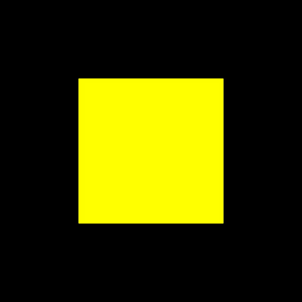 Figure 1
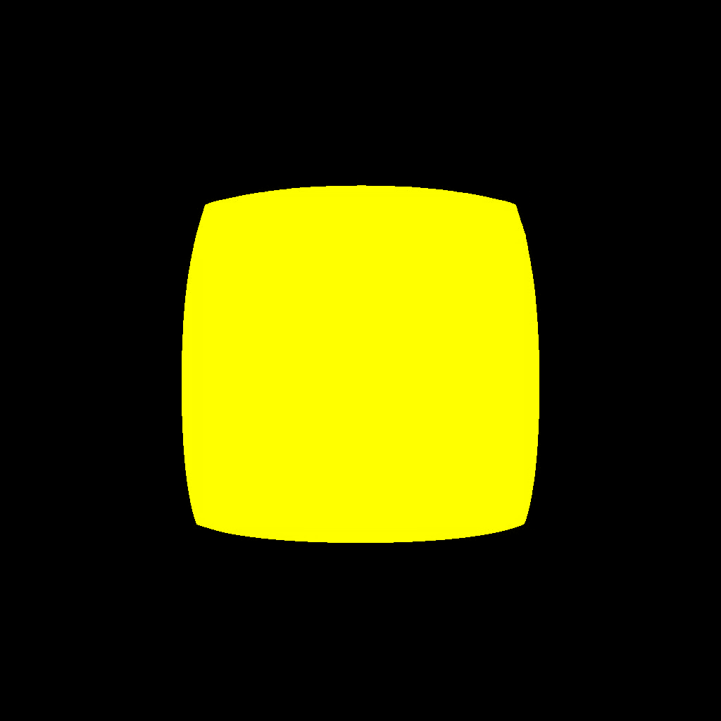 Figure 2
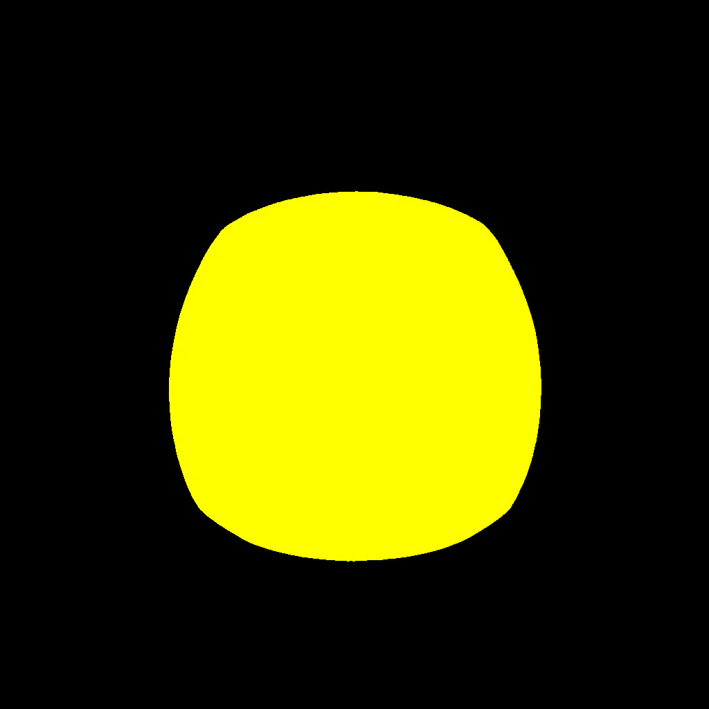 Figure 3
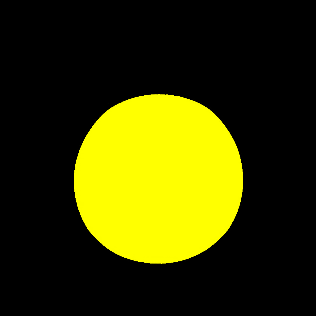 Figure 4
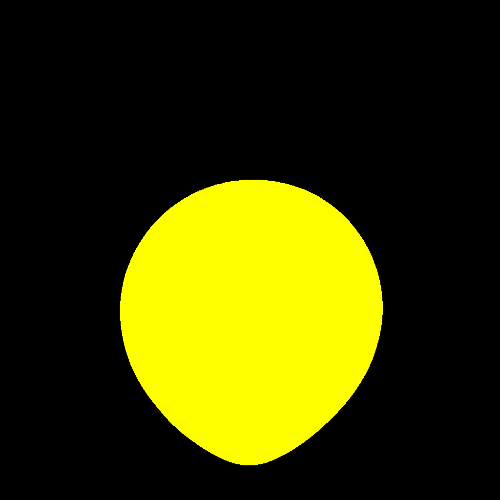 Figure 5
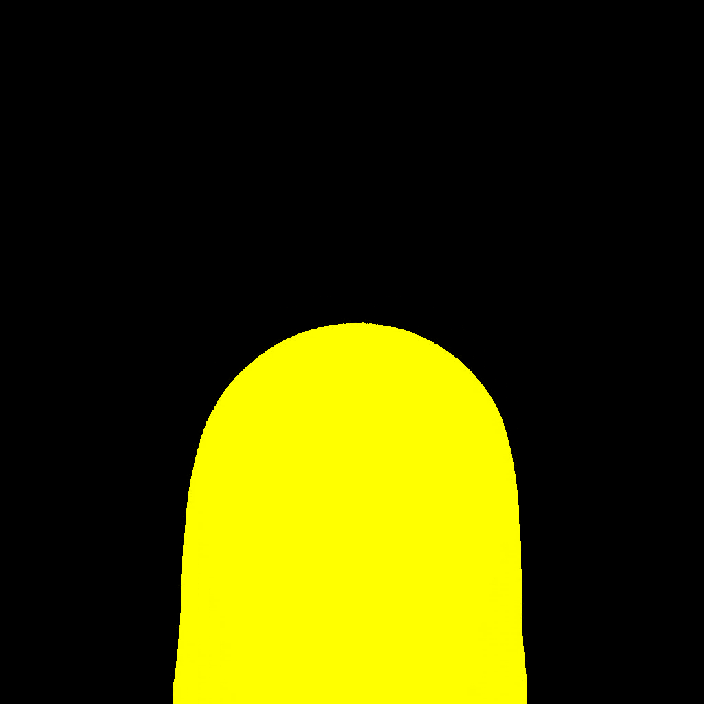 Figure 6
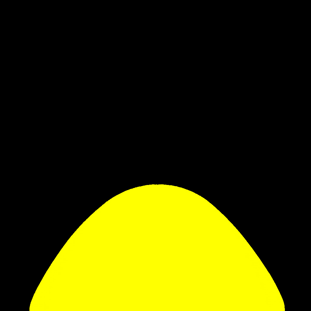 Figure 7
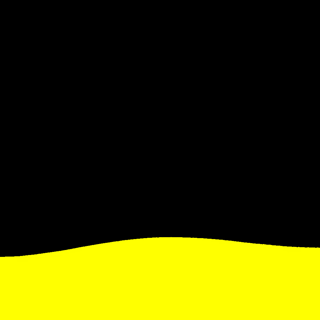 Figure 8
 Figure 9
 Figure 10
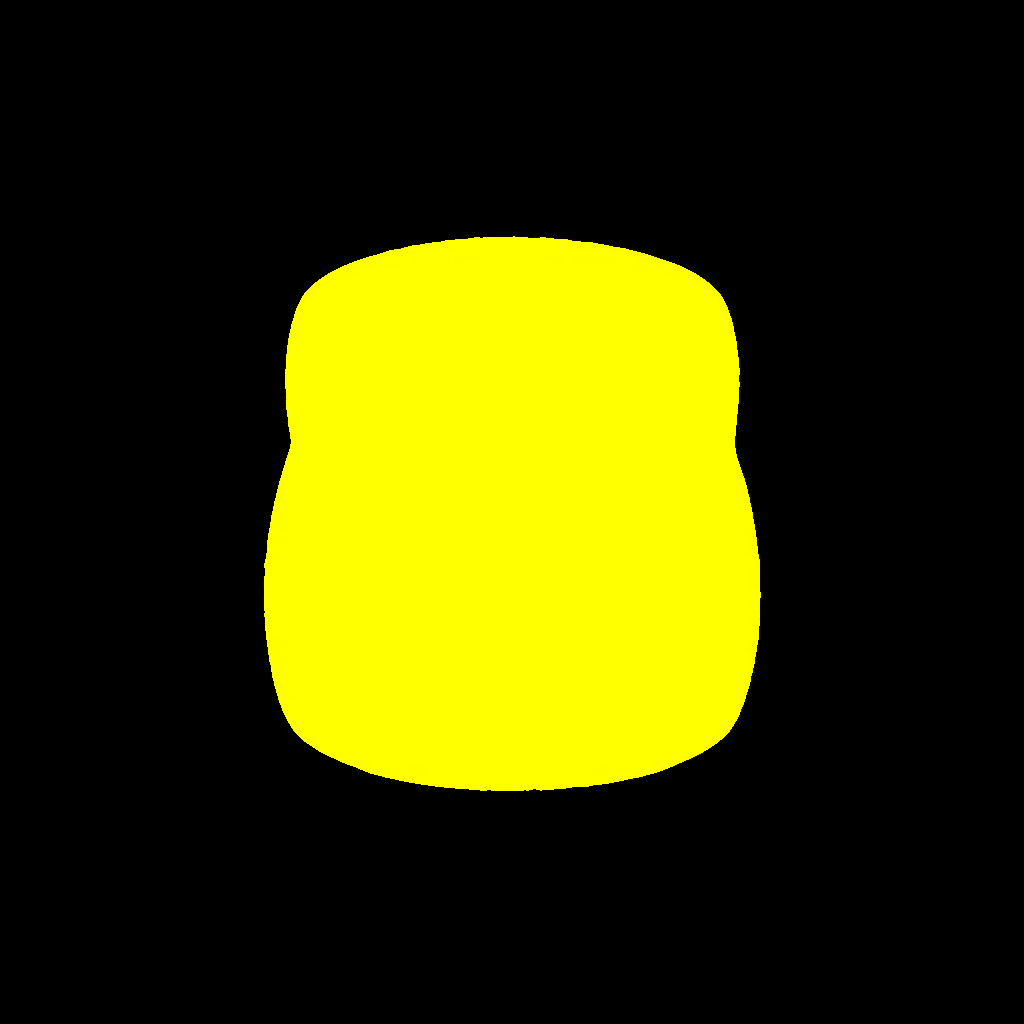 Figure 11
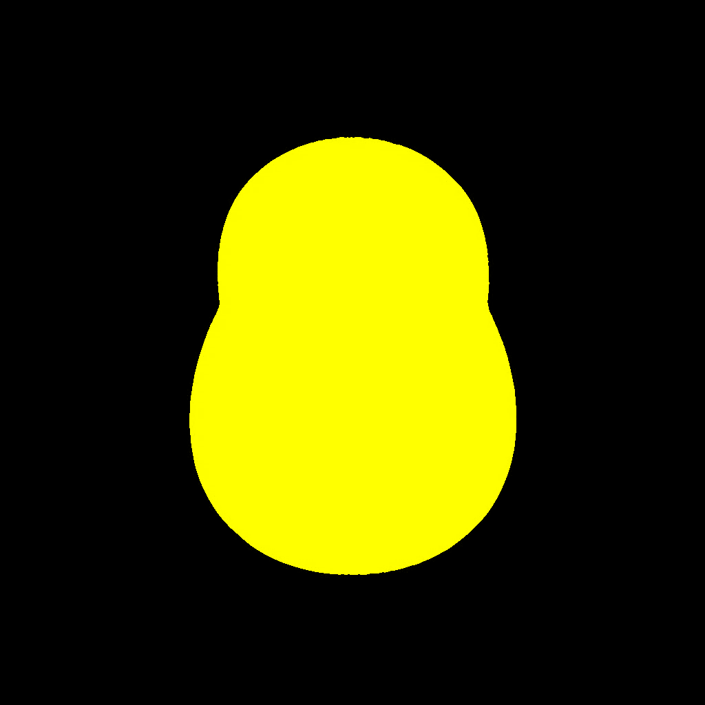 Figure 12
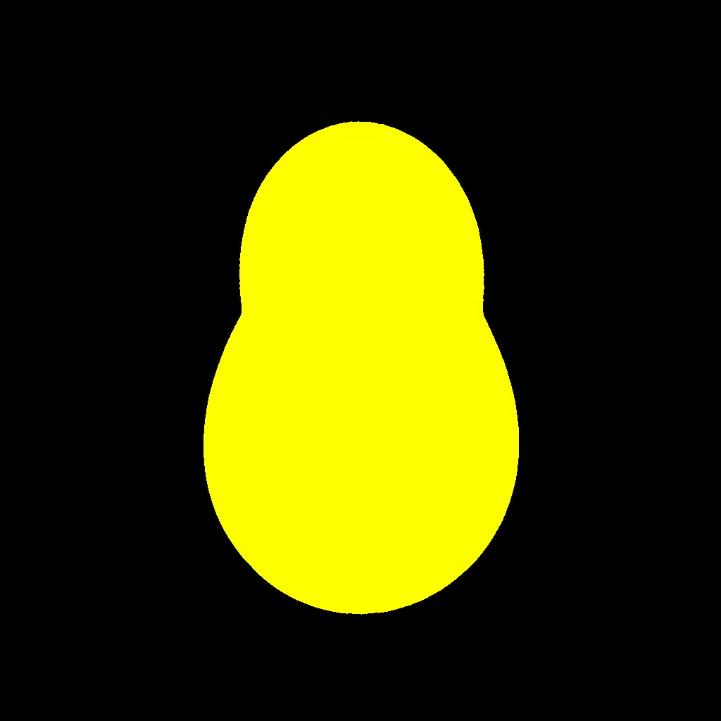 Figure 13
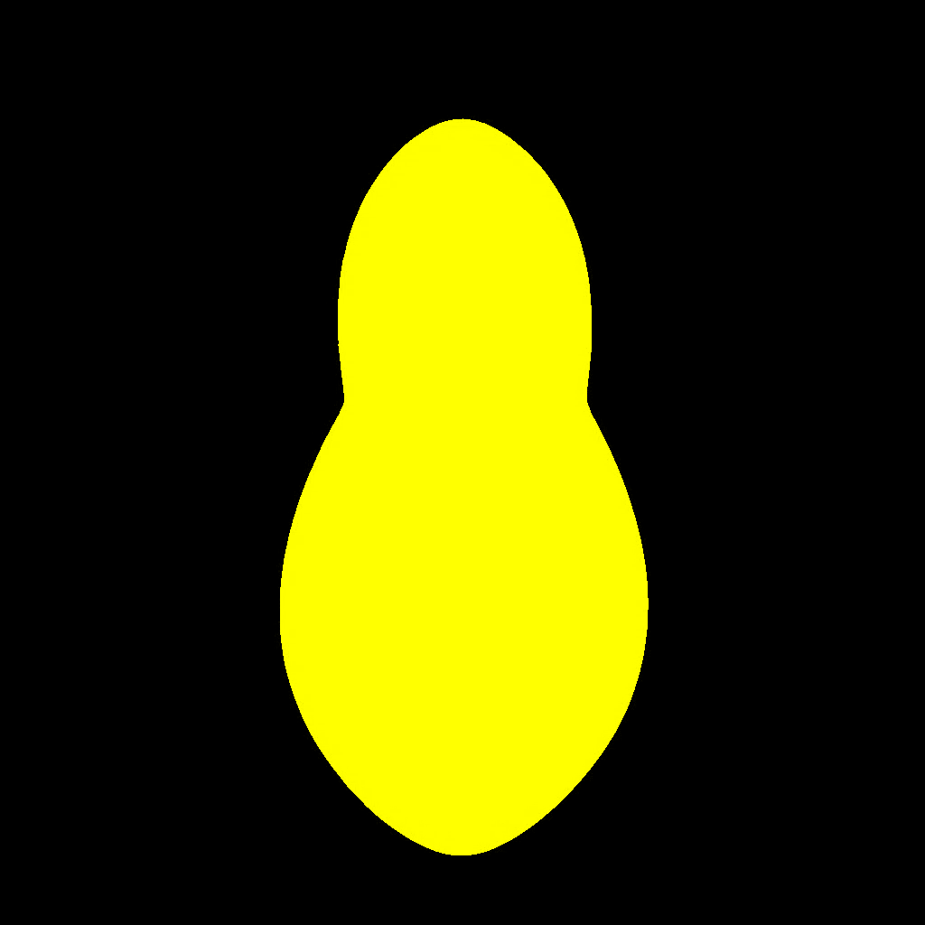 Figure 14
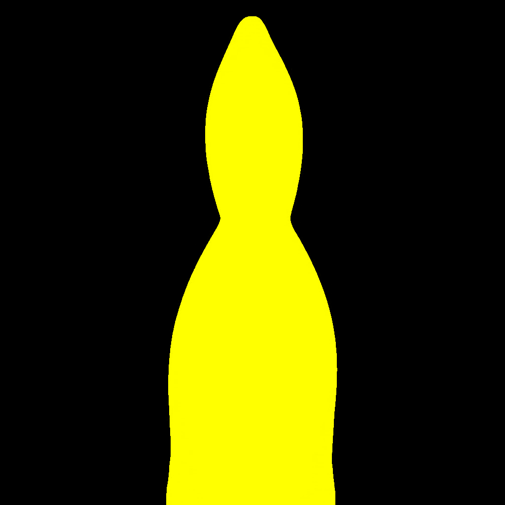 Figure 15
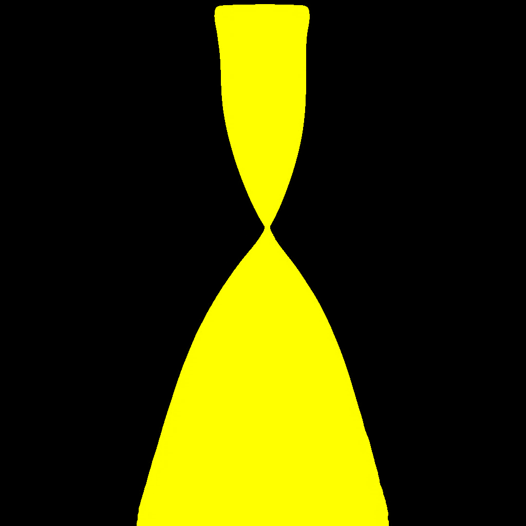 Figure 16
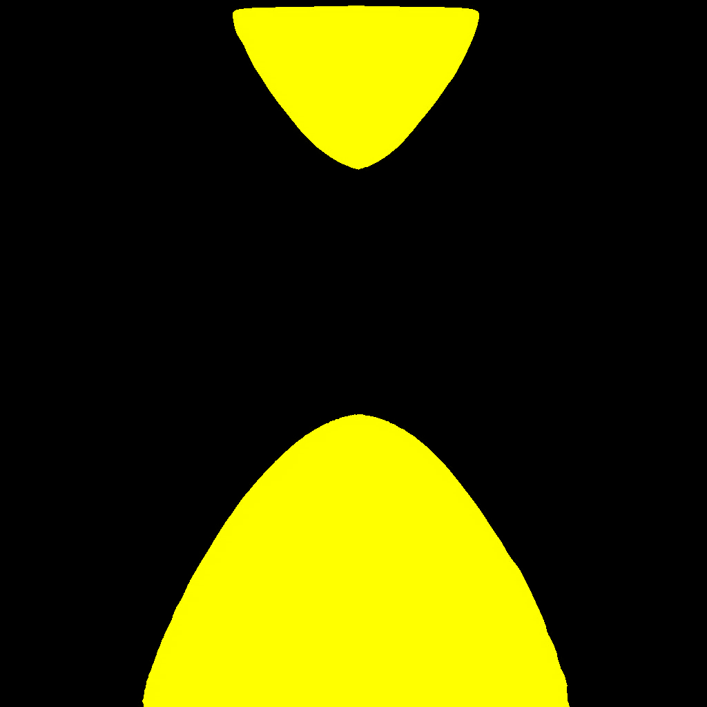 Figure 17
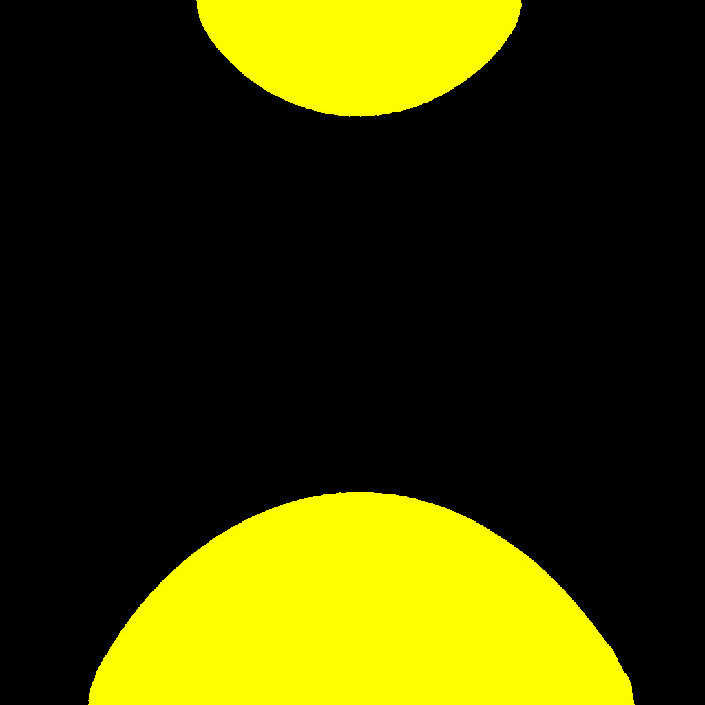 Figure 18
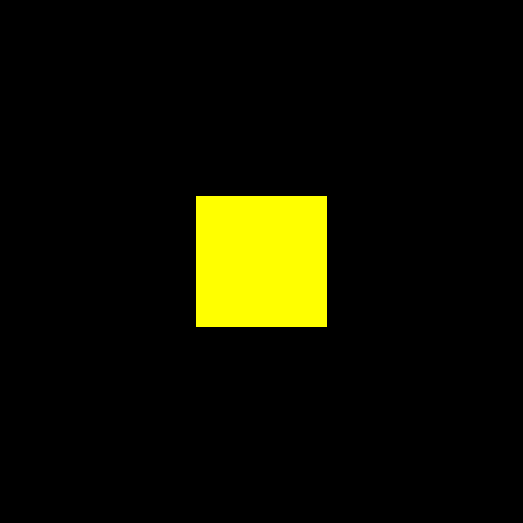 Figure 19
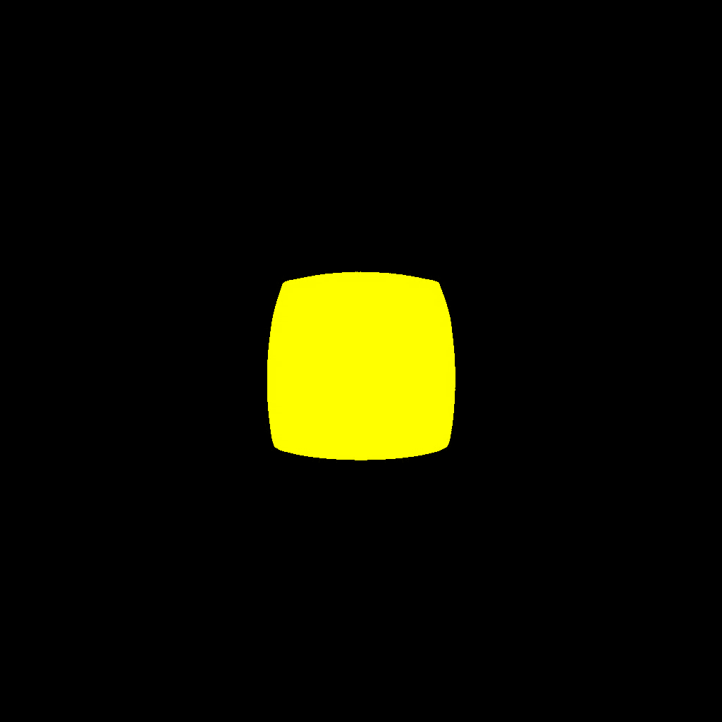 Figure 20
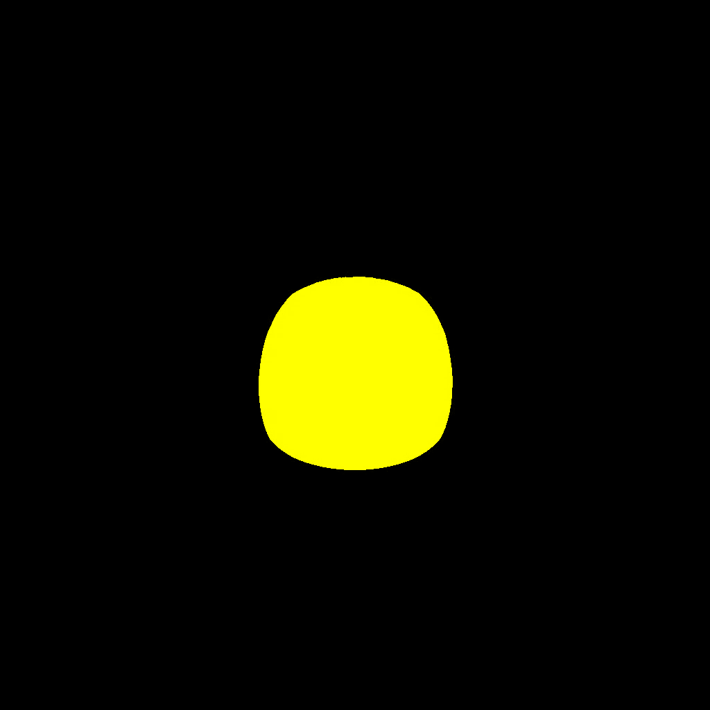 Figure 21
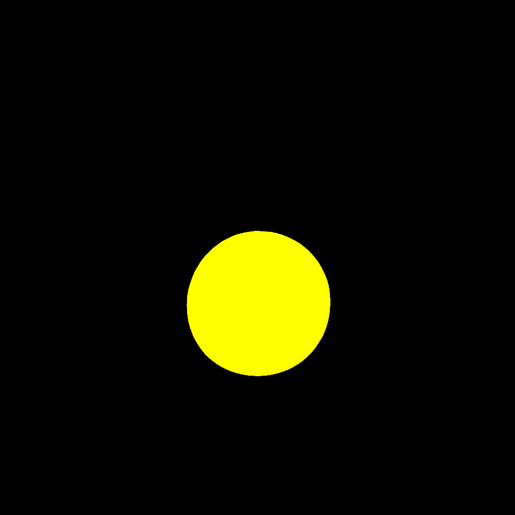 Figure 22
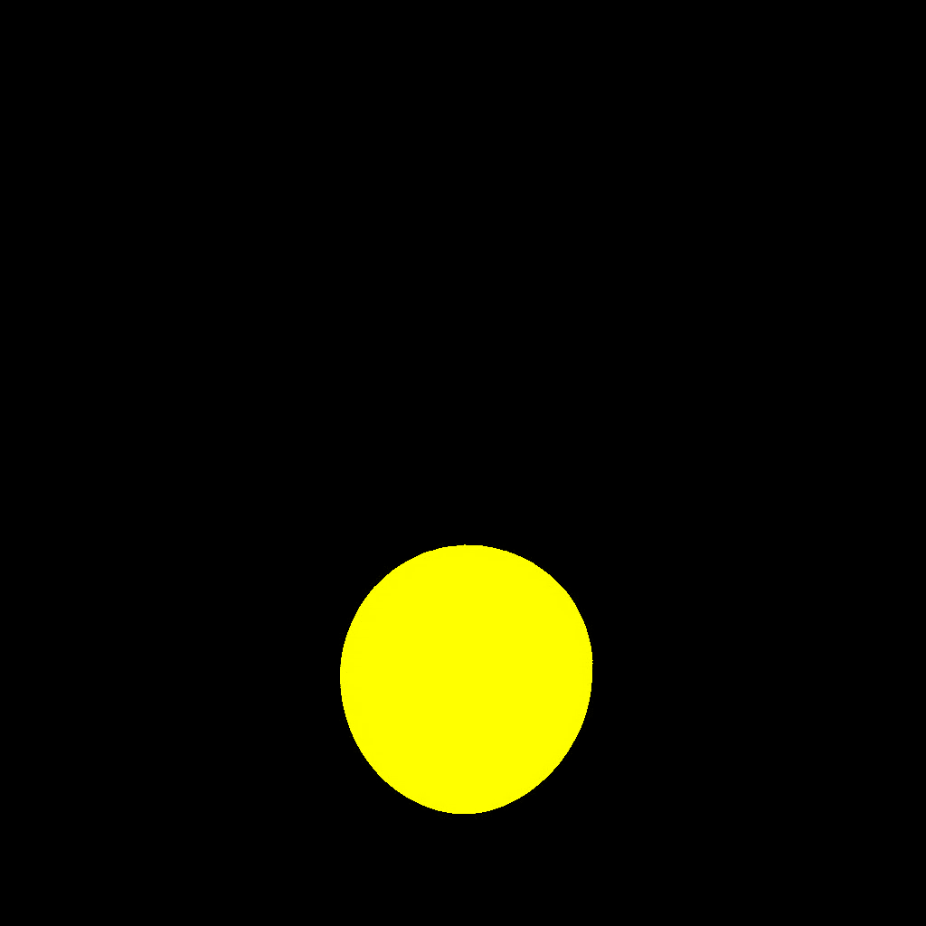 Figure 23
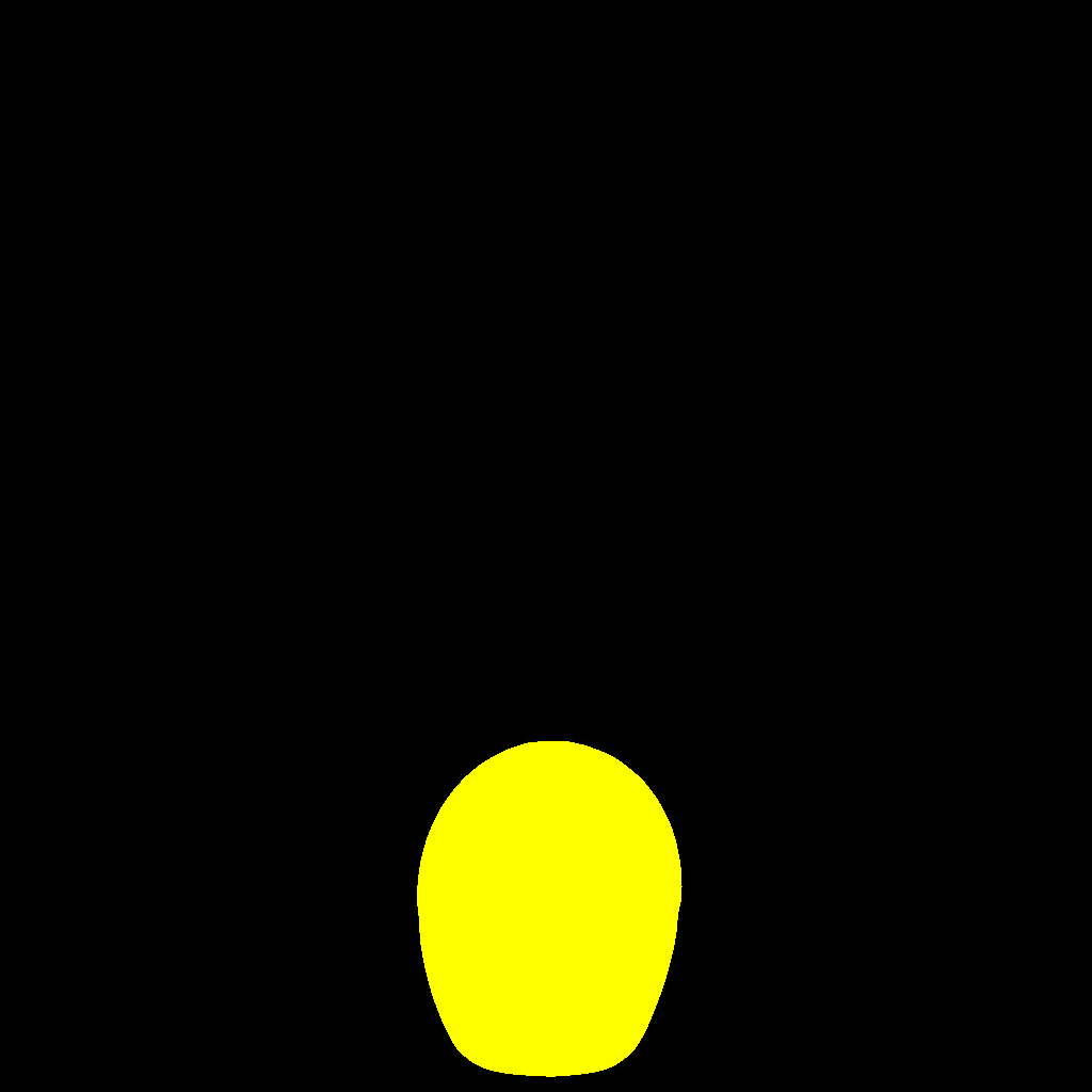 Figure 24
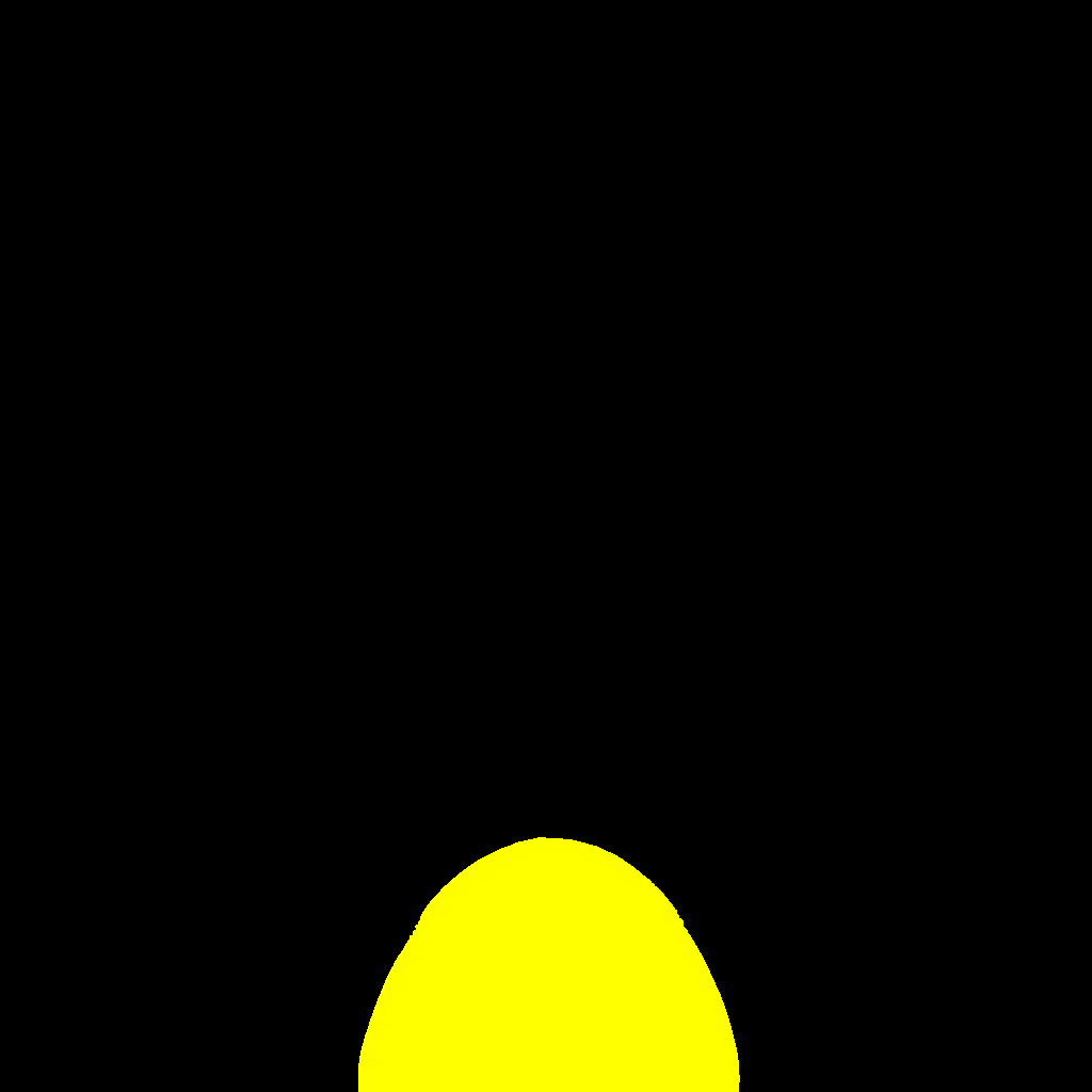 Figure 25
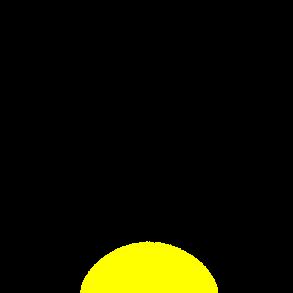 Figure 26
Peer Reviews
No public reviews on file for this paper yet. If you reviewed it on a platform where reviews are public (OpenReview, ICLR, NeurIPS, ICML), you can paste yours below so the community can read it here.
Videos
No videos yet. Explain this paper in a talk, walkthrough, or lecture? Add one.
Weak solutions to the Muskat problem with surface tension via optimal transport
Matt Jacobs
Department of Mathematics, UCLA, 520 Portola Plaza, Los Angeles, CA 90095, USA
,
Inwon Kim
Department of Mathematics, UCLA, 520 Portola Plaza, Los Angeles, CA 90095, USA
and
Alpár R. Mészáros
Department of Mathematical Sciences, Durham University, South Road, DH1 3LE, Durham, UK
Abstract.
Inspired by recent works on the threshold dynamics scheme for multi-phase mean curvature flow (by Esedoḡlu-Otto and Laux-Otto), we introduce a novel framework to approximate solutions of the Muskat problem with surface tension. Our approach is based on interpreting the Muskat problem as a gradient flow in a product Wasserstein space. This perspective allows us to construct weak solutions via a minimizing movements scheme. Rather than working directly with the singular surface tension force, we instead relax the perimeter functional with the heat content energy approximation of Esedoḡlu-Otto. The heat content energy allows us to show the convergence of the associated minimizing movement scheme in the Wasserstein space, and makes the scheme far more tractable for numerical simulations. Under a typical energy convergence assumption, we show that our scheme converges to weak solutions of the Muskat problem with surface tension. We then conclude the paper with a discussion on some numerical experiments and on equilibrium configurations.
1. Introduction
The Muskat problem was first introduced by Morris Muskat [30] as a model for the flow of two immiscible fluids through a porous medium. Since its introduction, this problem has received sustained attention in a variety of fields. It is used to model flows in oil reservoirs (water is injected into the oil well to drive oil extraction), and in hydrology to model flows of groundwater through aquifers.
In this paper we are interested in obtaining the global existence of weak solutions for the Muskat problem with surface tension, based on its gradient flow structure. We begin by introducing a variational formulation of the problem, which will motivate our subsequent analysis. The fluid evolution can be written as Darcy’s law
[TABLE]
coupled with the continuity equation
[TABLE]
where is the velocity of phase , is the collection of relative concentrations for each phase, denotes the spacial gradient of the classical first variation of the free energy with respect to , and () denotes constant mobilities. For convenience, throughout the rest of the paper, we will refer to as a collection of density functions; however, one should note that only encodes information about the volume occupied by the fluids and nothing about their mass.
The physical setting for our problem is a bounded, convex open domain with smooth boundary. We shall suppose that the two fluids fill the entire domain, and that they are confined to for all time. We then take the internal energy to be a sum of three distinct terms:
[TABLE]
The first term in the energy, describing incompressibility and containment of the fluids, is given by
[TABLE]
The immiscibility of the fluids and the surface tension force arise from the highly non-convex interaction energy
[TABLE]
where denotes the total variation of in and is a surface tension constant. Finally, denotes the potential energy of the fluid configuration, i.e.
[TABLE]
where are given Lipschitz continuous potentials. A typical example is when one assumes these to be gravitational potentials, i.e.
[TABLE]
where ’s are proportional to the specific gravity of each fluid.
Although the internal energy is singular, when and are separated by a smooth interface , one can formulate a classical solution to the Muskat problem equations (1-2). In the classical solution, the flow is driven by the pressure variables for each phase, which are Lagrange multipliers generated by above. The continuity equation becomes
[TABLE]
and the pressure is determined by solving the free boundary problem
[TABLE]
where denotes the mean curvature of , oriented to be positive when is convex at the point, denotes the outer normal along and along , and denotes the co-normal vector orthogonal to and tangential to . Note that the final condition relating the co-normal vector at to the normal vector of implies that must meet orthogonally (see Lemma 3.1 and Remark 3.2 for the weak formulation of this condition). To summarize the ideas in the formal derivation of (MP1)-(MP2) from (1)-(2) using the definition of , we heuristically have , while the contribution of will act only on in the form of the curvature .
Problems like (MP2) received a lot of attention in the past decades. Most of the works focus on the zero surface tension model () and well-posedness of regular solutions with graph property [2, 6, 8, 9, 10]. In the presence of surface tension, the problem has stronger regularity properties in stable settings [34], but still, topological singularities can occur in finite time, for instance when heavier fluid is placed on top of the lighter one [14]. Thus, our aim is to construct global-in-time weak solutions to the Muskat problem (MP2), which exist past the formation of singularities.
To construct global-in-time solutions, we exploit the gradient flow structure of the Muskat problem. As noted by Otto in [31, 32], Darcy’s law can be approximated by the Euler-Lagrange equation for the minimizing movements scheme (or JKO [19] scheme) with time step size ,
[TABLE]
where denotes the 2-Wasserstein or 2-Monge-Kantorovich distance. In this context, the squared distance has a physical interpretation as the energy dissipated by friction as the fluids flow through the porous media.
Let us note that Wasserstein gradient flows of energies involving total variation terms have been considered before in the literature, though only in the case of one phase models (see e.g. [26, 5]), and hence with no incompressibility or interaction constraints. As a result, the techniques developed in those papers do not appear to be applicable here — the constrained two phase setting adds many additional difficulties.
Indeed, it is not easy to obtain a complete characterization of the solutions to the minimizing movements problem (7). The interaction energy (5) is sufficiently non-convex that problem (7) is non-convex for any . As a result, one must be careful in using duality to introduce the pressure as a Lagrange multiplier. Furthermore, we are interested in developing a scheme which could be used for numerical implementations. The formulation (7) is poorly suited for numerical methods. Optimizing over the non-convex constraint set is extremely difficult. For these reasons, we instead consider a relaxed version of minimizing movements scheme inspired by [13] and [22].
Approximation of the perimeter by the Heat Content
In our analysis, we replace the interaction energy in (7) by the heat content energy
[TABLE]
Here stands for the standard heat kernel (with mean 0 and variance ) and the densities are assumed to be defined on all of by extending them to zero off of . Let us notice that in [13] and [22], for similar purposes the authors use periodic extensions. The analysis in both cases and the validity of results using both kinds of extensions is essentially the same.
Dating back to the work of De Giorgi, approximate perimeter energies have been used in the literature to study geometric variational problems (see for instance [29] and [1]). The use of the heat content energy to study the multi-phase mean curvature flow was first introduced by Esedoḡlu and Otto in [13]. It was observed in [13] that the threshold dynamics, a well known numerical scheme for mean curvature motion introduced by Merriman, Bence, and Osher [28], is precisely a minimizing movements scheme for the heat content energy. Esedoḡlu and Otto also showed that -converges (with respect to the topology) to as . Building off of these results, Laux and Otto showed in [22] that under an energy convergence assumption, the threshold dynamics scheme produces weak solutions to the multi-phase motion by mean curvature in the limit .
Our goal is to consider such a framework in the context of the Muskat problem by studying the minimizing movements scheme
[TABLE]
where we used the notation
[TABLE]
As we alluded above, the scheme (9) has a number of numerical advantages over (7). Unlike which is neither convex nor concave, the heat content is a strictly concave functional of the densities. This concavity can be exploited to simplify numerical implementations, along the same lines as the linearization trick noted in Subsection 5.1 of [13]. After applying this trick, the resulting variational problem becomes convex, and thus, can be efficiently solved using the recently introduced back-and-forth method [18]. See Figures 1-3, for a demonstration of the numerical performance of the scheme.
Although the heat content in principle allows mixing of the phases, we shall show that the discrete in time solutions constructed by the JKO scheme always stay unmixed with a sharp interface between the phases for all time (see Proposition 2.3 below). This phenomenon is due to the fact that behaves like a strictly concave functional (see Lemma 2.2). Thus, one retains the essential properties of the Muskat problem evolution.
In the context of the Muskat problem, the heat content also has a natural physical interpretation. In a discrete statistical mechanics model with particles, surface tension can be seen to arise from short range interactions between particles in different phases (cf. [17]). Typically, the discrete surface tension takes the form
[TABLE]
where is the particle index in each phase , is some decreasing function, and is the location of particle ([17]). By taking the limit in above formula, one obtains an analogue of the heat content energy where the kernel is replaced with . Here it is worth noting that we choose to work with the heat kernel for computational convenience, indeed a different choice of kernel may be more physically relevant.
Finally, let us also emphasize that the heat content approach can be naturally extended to the multiphase Muskat problem evolution (with any number of phases), without incurring any additional difficulties (just as in the case of [13] and [22]). This includes scenarios where the surface tension force depends on the phases that are interacting [13]. To present our ideas in the simplest possible way, we do not pursue the multiphase case in this paper.
Statement of our main results
From the relaxed minimizing movements scheme (9), we obtain a sequence of discrete in time approximations to the Muskat flow. When we take the time step and the heat content approximation parameter to zero together, we hope to recover weak solutions to the Muskat problem. Our main results show that this is indeed the case under the assumption that there is no loss of perimeter when passing from discrete to continuous solutions. For the precise statements of the convergence results we refer to Theorem 3.1 and Theorem 3.2. In addition, we show that our weak formulation (see Definition 3.1) encodes all of the conditions in (MP1)-(MP2) (see Lemma 3.1 and Remark 3.2).
Theorem 1.1**.**
Let be a fixed time horizon, let be fixed and let be the discrete in time interpolations of the densities obtained from the minimizing movements scheme (9). Let moreover stand for the discrete in time interpolations between the scalar pressure fields, obtained as Lagrange multipliers associated to the incompressibility constraint in (9). Then
- •
There exists a family of measurable sets such that and .
- •
There exists () such that as and along a subsequence strongly in . Moreover, and they are also characteristic functions that sum up to one, i.e.
[TABLE]
for a measurable family of sets which are of finite perimeter.
- •
There exists a scalar pressure field such that along a subsequence weakly-* in as .*
- •
Finally, under the assumption of energy convergence
[TABLE]
* with solves, in the weak sense (see Definition 3.1), the problem (MP1)-(MP2). Here formally corresponds to .*
It is challenging to study qualitative or geometric properties of our solutions. We will illustrate heuristically in Section 4 that, even for global minimizers of the energy, there are diverse possibilities depending on the values of the specific gravity and volumes of the two phases. This is verified with several numerical simulations in Section 4.1.
Remarks on our results
- (1)
Let us underline the fact that our discrete-time scheme (9) produces minimizers that are characteristic functions of a partition of . To prove this fact, we exploit the strict concavity of the heat content along the admissible set. This seems to be an interesting property in its own right, and ensures that numerical implementations of the scheme maintain a sharp interface at every time step.
- (2)
From the point of view of Wasserstein gradient flows, an interesting remark on our results is that while one cannot expect strong compactness for the interpolated densities in the case when is fixed and , when sending both parameters to 0 in the same time, we regain the strong compactness. This phenomenon is mainly due to the fact that in the limit as we recover total variation estimates on the densities. This compactness is obtained via a standard Aubin-Lions type argument.
- (3)
The energy convergence assumption (EC) is rather natural and the same as the ones given in [22] and [23]. This assumption ensures that there is no sudden loss of boundary between phases in the limit . If there is a loss of interface then one cannot obtain weak solutions. Indeed, if two components of the support of merge into each other and remove a sizable part of its boundary, one can expect a discontinuous change of the pressure term in the entire domain , creating an inconsistency between the discrete and limiting evolutions.
Replacing the assumption with a direct argument has been discussed for mean curvature flows [40, 11]. Unfortunately, these results rely strongly on certain properties of the mean curvature flow (especially the comparison principle), which do not hold for fourth order equations like the Muskat problem.
There are also results in the literature [24, 35] which eliminate the assumption for third order curvature driven flows (specifically the Stefan problem and the Mullins-Sekerka flow respectively). However, the solutions constructed in [24] are discontinuous in time (the interface may experience sudden jumps in time) and the formulation in [35] only keeps track of the regular part of the interface. Let us also note that the Stefan problem and the Mullins-Sekerka flow are not similar to the Muskat problem. In particular, the jump condition for the pressure across the interface is different for the Muskat problem, which leads to qualitatively different behavior.
Paper summary
The rest of the paper is organized as follows. In Section 2, we derive the basic properties of the minimizing movements scheme (9) and construct our discrete-time quantities. We begin by showing that solutions to the minimization problem are characteristic functions at every time step of the discrete scheme. We then derive the existence of pressure as a Lagrange multiplier for the incompressibility constraint and obtain the Euler-Lagrange equation for the minimization problem. Our derivation of these equations were inspired by previous results from [12, 27, 21, 20]. In particular, the definition of the discrete in time pressure variable is very much inspired by [27].
In Section 3, we take and to zero together to obtain weak solutions to the Muskat problem, under the assumption that the internal energy of the discrete solutions converges to the internal energy of the limiting solutions. The main task in this section amounts to showing that one can pass to the limit in the Euler-Lagrange equation obtained in Section 2. This can be done using the standard theory for Wasserstein gradient flows if is held fixed. However, the joint limit, , requires an adaptation of the arguments of [22] to the case of Wasserstein gradient flows. Let us underline that one can rely entirely on the results of [22] to pass to the limit the weak curvature equation. An adaptation of the Aubin-Lions type argument from [22] can be done to get compactness of the density terms. The only difference here is that we are using as metric while in [22] a different metric is used, but this does not impose crucial difficulties. An interesting link to the flow-exchange technique introduced in [26], which is a typical tool for gradient flows, is also pointed out. Last, we developed the necessary estimates and compactness results on the pressure terms. These are new and clearly were not present in the setting of mean curvature flows. The compactness that we get on the pressure is in the sense of distributions.
Finally, in Section 4, we conclude the paper with a demonstration of the numerical method on several examples and a discussion on the global minimizers of the approximated internal energy associated to the Muskat problem. While this discussion remains at the heuristic level, our conjectures are supported by the equilibrium states attained in our numerical experiments (c.f. Figures 1-3). We end the paper with an appendix section, where we recall the results from [22] that are used when passing to the limit the weak curvature equation.
2. The Wasserstein minimizing movements scheme for the heat content
2.1. Some preliminary results
Recall that the setting for our problem is a smooth convex domain and without loss of generality by scaling we assume that . By we denote the space of Borel probability measures on supported on . stands for the elements of that are absolutely continuous with respect to .
Let be given Lipschitz potentials and let us recall the definition of the potential energy , given as
[TABLE]
Let . We consider the heat content defied in (8), using the standard heat kernel , i.e.
[TABLE]
We also use the notations to denote and We have the following preliminary results.
Lemma 2.1**.**
Let be defined as in (8). We have the following properties.
- (1)
* is bounded from below and continuous w.r.t. the weak- convergence on *
- (2)
* displacement -convex on , with .*
Proof.
(1) Is immediate by the definition of .
To show (2), it is enough to show that the function is -convex in the classical sense for some . We have
[TABLE]
Since the matrix is positive semidefinite for any , setting , we have that the matrix is positive semidefinite for any which implies in particular that is -convex.
We conclude similarly as in [12, Lemma 2.1] the displacement -convexity of on ∎
Lemma 2.2**.**
If denotes the set of pairs such that a.e. in , then the heat content is strictly concave along line segments in .
Proof.
For any pair we may write . Thus, extending the densities by [math] outside of , we have
[TABLE]
Ignoring the constant multiples, both terms can be expressed conveniently in the Fourier domain:
[TABLE]
Now the strict concavity follows immediately as for all . ∎
2.2. The minimizing movements scheme
Now we are ready to discuss the minimizing movements scheme. Our first result confirms the existence of minimizers, and shows that any minimizing configuration is a completely unmixed partition of the domain. As we will see, the phases stay unmixed thanks to the concavity of the heat content.
Proposition 2.3**.**
Suppose that and let and . Then the set of minimizers of the problem
[TABLE]
is non-empty and any solution is the characteristic function of a partition of .
Proof.
The existence of a solution of the optimization problem is an easy consequence of the weak lower semicontinuity of the objective functional and the weak- compactness of . Let us remark that the constraint a.e. is closed under weak convergence, since
To show that an arbitrary solution is the characteristic functions of a partition of , let us rewrite equivalently the minimization problem in terms of transport plans . Recall that is a plan between and , whenever
[TABLE]
for any Since we are always working with measures that are absolutely continuous w.r.t. , in the new minimization problem below, as we will see, we can restrict our search to plans that have absolutely continuous marginals w.r.t. For a measure , we use the notation and to denote its marginals (here stand for the canonical projections from onto ).
Thus, we aim to solve
[TABLE]
Here we denote
[TABLE]
We define moreover
[TABLE]
and
[TABLE]
where we have extended the second marginals of by 0 outside of .
The minimization is carried out over a weakly compact set and is weakly lower semicontinuous and bounded below, thus minimizers exist. If is a minimizer of (12) then we can construct a minimizer of the original problem by taking .
Now we consider the properties of minimizers. Clearly, is Gâteaux differentiable at in the sense that there exists such that
[TABLE]
where is any admissible perturbation of Similarly, as the other terms in the definition of are linear in , these are in the same way differentiable, therefore is Gâteaux differentiable in this sense.
From Lemma 2.2 it follows that is concave along line segments (), where is a feasible point and is a feasible direction at i.e.
[TABLE]
and for some
[TABLE]
in the sense of signed measures, for all . Furthermore, it follows from Lemma 2.2 that is strictly concave on line segments , if for some the marginal is not [math] for almost every . Therefore, if is a minimizer and is a feasible direction at with at least one non-trivial marginal then
[TABLE]
where stands for the first variation of at defined as is (13).
Let be a feasible solution and let . Now suppose that there exists such that the set has positive measure. Partition into two sets of equal measure. Then there exist measure preserving maps and such that and are the identity almost everywhere on their respective domains (for example one may choose to be the optimal transport map between the densities and and ). Now we construct a feasible direction at as follows. Let for and we define the signed measures as
[TABLE]
i.e.
[TABLE]
and
[TABLE]
i.e.
[TABLE]
for any
Since a.e. on we see that has a nontrivial marginal.
Let us now check that is feasible, i.e. it satisfies (14) and (15). If then defines a non-negative measure. Next, we check that satisfies for a.e. and and for a.e. . For , we have
[TABLE]
and
[TABLE]
where we have used that both and are measure preserving between and and vice-versa, respectively. Let us notice that these arguments also show (by taking ) that
[TABLE]
Now, for we have
[TABLE]
Note that our arguments in fact show that is also a feasible direction at . have nontrivial marginals, and it is not possible to have both and . Therefore, cannot be a minimizer. This allows us to conclude that for any minimizer of the original problem each density takes values almost everywhere.
∎
2.3. Optimality conditions and construction of the pressure variables
In the next Lemma, we give a more complete characterization of the minimizers in terms of certain necessary inequalities. In particular, this is the first place where we see the appearance of the pressure variable, which plays an essential role in all of the subsequent analysis. Note that for convenience we express this result using the notation
Lemma 2.4**.**
Let be an optimizer in (11) and let a pair of probability measures such that a.e. Then,
- (i)
we have the following optimality condition
[TABLE]
for a suitable pair of Kantorovich potentials in the optimal transport of onto and onto , respectively.
- (ii)
there exists a function that is Lipschitz continuous on , and is such that for any probability densities with a.e. we have
[TABLE]
moreover, we have
[TABLE]
Proof.
Let be a pair of probability measures such that a.e. For let us consider the competitors , which by construction satisfy the constraint.
By optimality, we have
[TABLE]
Using the exact same argument as in [27, Lemma 3.1] to develop the Wasserstein part on the one hand and the first variations of and on the other hand, we find (16).
For (ii) (similarly as in [21, Proposition 4.7]), let us notice first that (16) can be written in the form
[TABLE]
where is such that and for . We know from Proposition 2.3 that forms a partition of . Therefore, we must take on , and on (and vice-versa for ). To preserve the constraint and the mass of each density, we must also take a.e. and .
Now if we set , we find that
[TABLE]
for any with 0 mean such that a.e. on . This implies that there exist constants such that
[TABLE]
[TABLE]
From here, we can define the pressure variable as
[TABLE]
Since the Kantorovich potentials are Lipschitz continuous and the other terms are smooth, we find that is Lipschitz continuous (note this regularity may degenerate as ). By construction, clearly satisfies the inequality in (17), and in particular the value of the l.h.s. is equal to zero. Since the functions under consideration are all Lipschitz continuous, we obtain (18). ∎
2.4. Continuous in time solutions for fixed
Now we are ready to begin constructing time interpolations from the discrete scheme. In this section we restrict ourselves to the case where is held fixed. In this special case, we can use standard arguments from the theory of Wasserstein gradient flows to obtain continuous in time equations in the limit . When is held fixed, we have strong compactness on the pressure term. However, similarly to the models in [20, 21], we will lack strong compactness on the density variables, which would mean that in the limit when , only a weaker version of the system will be available (see (25)). Let us also note that later on in Section 3, we will need some of the pressure estimates provided below when we take to zero along with .
Let be a given time horizon and and such that Let be fixed. By now, it is standard how to construct weak solutions to PDEs that have gradient flow structure, using minimizing movement schemes as
[TABLE]
Let be defined as
[TABLE]
We define the corresponding velocities, pressures and momentum variables as
[TABLE]
where and are defined in Lemma 2.4. Following the same steps as in [20, 27], the analysis boils down to obtain a sufficient amount of uniform (in ) estimates and compactness for the previously obtained functions, then pass to the limit
Also, as additional tools we construct the corresponding continuous in time (geodesic) interpolations between the densities and the corresponding velocities and momentum variables, . We refer to [20, Section 3.1] (see also [27, 37]) for the precise construction. In particular, as a consequence of this construction, we have
[TABLE]
in the sense of distribution on . Let us comment on the role of the geodesic interpolations. These interpolations (beside the more standard piecewise constant ones) in the context of –gradient flows were first used by Santambrogio (see the discussion in [37, Section 8.3]). Their role is the following: for any , these interpolations, since pieces of geodesic curves, by definition solve continuity equations. Since the piecewise constant interpolations match the geodesic ones at node points , if both of them converge, they need to converge to the same limit. Therefore, one automatically has a continuity equation as the limit of piecewise constant interpolations. An alternative way (which is more often used in the literature) would be to say that the piecewise constant interpolations solve a continuity equation up to an error term, then one would need to show that this error term is converging to zero as the time discretization parameter tends to zero.
Based on the same techniques as in [27, 20], it is easy to obtain the following estimates.
Lemma 2.5**.**
Let and be the previously constructed piecewise constant and continuous in time interpolations, respectively. Then there exists independent of and depending only on such that
- (i)
* and for any Moreover, up to passing to subsequences and converge (uniformly with respect to ) as to the same limit.*
- (ii)
* is uniformly bounded in *
- (iii)
* and are uniformly bounded in and up to passing to subsequences they have the same distributional limits as .*
- (iv)
**
- (v)
* for any with and any .*
- (vi)
, and as a consequence, is uniformly bounded in and is uniformly bounded in by a constant of the form
- (vii)
* is uniformly bounded in independently of and . In particular, is uniformly bounded in and defines a uniformly bounded distribution of order one, for a.e. .*
Proof.
Let us notice that the proofs of point (i), (ii) and (iii) follow the exact same lines of the proofs of [27, Lemma 3.3] and [20, Lemma 3.3], so we omit them.
From Proposition 2.3 we know that that ’s are characteristic functions, therefore the proofs of (iv) and (v) follow the exact same lines as the proof of [22, Lemma 2.4.].
Let us give the details on (vi). From the identities (18) from Lemma 2.4, we have that there exists (independent of , which might increase from one inequality to the next) such that
[TABLE]
where we have used the uniform bounds on from the previous points and
[TABLE]
Since a.e., this previous bound implies that is uniformly bounded in As a consequence of Poincaré’s inequality, we have that is uniformly bounded in . Both uniform bounds have the form
To show (vii), let . Fix . Taking the inner product of both sides in (18) with and integrating on w.r.t. (we drop the dependence on in the notation of ), we obtain
[TABLE]
and interchanging the roles of and , we get
[TABLE]
First, we have
[TABLE]
where in the second and third equalities we have used the change of variables and , respectively and the fundamental theorem of calculus in the last equality. Now, since
[TABLE]
for some universal constants , by the previous chain of equalities, we obtain
[TABLE]
where, in the last inequality we used the monotonicity of along the sequence .
Furthermore, we have that
[TABLE]
and
[TABLE]
Using the fact that we have piecewise constant interpolations, integrating the last equality in time on , we get
[TABLE]
Now, adding together (23) and (24), then integrating in time on and using (ii), we obtain
[TABLE]
where the constant is independent of and . The thesis of follows. ∎
Now we can use the above pressure estimates to derive a system of continuous in time equations in the limit when is held fixed.
Theorem 2.1**.**
Let , such that a.e. There exists , , and such that a.e. in , a.e. in and the system
[TABLE]
is satisfied in the sense of distributions on
It remains open whether in the previous theorem we have strong convergence in as , and in particular whether one can claim that
Proof of Theorem 2.1.
Using the uniform (in ) estimates in Lemma 2.5, we have the existence of , such that up to passing to a subsequence, both and converge to them uniformly in time, w.r.t. .
Since is uniformly bounded in , there exists such that up to passing to a subsequence, , weakly in and , weakly in as .
We only need to identify the limits of the momentum variables . From the weak convergence of the density variables, we have that up to passing to a subsequence, , as and similarly , and , as as vector measures.
Furthermore, since is uniformly bounded in , there exists , such that up to passing to a subsequence weakly in , as .
Last, by the previous arguments, we have
[TABLE]
as in Therefore, the thesis of the theorem follows.
∎
It is open whether the continuum in time densities in Theorem 2.1 are characteristic functions. Indeed, since we can only guarantee that the discrete densities converge weakly to the continuum densities, the characteristic function property may be lost in the limit. We point out that due to the energy bounds, the densities are “almost” characteristic functions, i.e. we have
Lemma 2.6**.**
For given as above with fixed, for any we have
[TABLE]
Proof.
Let us set , the other case will be parallel. We have
[TABLE]
By Jensen’s inequality, the above is smaller than
[TABLE]
We then estimate
[TABLE]
Since and take values in , we have . Applying these inequalities, the result follows. ∎
3. Muskat flow with surface tension
In this section, we complete the proof of Theorem 1.1 and show that when goes to zero along with , the time interpolated minimizing movements scheme constructed in (21)-(22) converges to a weak formulation of the Muskat problem with surface tension under the energy convergence assumption (EC). This amounts to showing that each quantity in the system of Euler-Lagrange equations given in (18) converges (in an appropriate sense) to the correct limiting object. In particular, we will need strong convergence of the density functions in . To obtain the necessary compactness for strong convergence, we develop an adaptation of an Aubin-Lions type lemma in Proposition 3.2. We then conclude our result by verifying the convergence of the Euler-Lagrange equations to the weak formulation of the Muskat problem in a similar manner to the approach in [22].
Before we introduce the weak formulation of the Muskat problem, let us recall the classical formulation of the problem. When the two phases are separated by a smooth interface , the Muskat problem is given by the continuity equation
[TABLE]
along with the free boundary problem for the pressure
[TABLE]
where is the mean curvature of , oriented to be positive when is convex at the point. The weak formulation of the Muskat problem with surface tension is provided in Definition 3.1 below.
Definition 3.1**.**
We say that is a weak solution to the Muskat problem with surface tension, if for a.e. , , and a.e., , and for any and for any vector field with zero normal component on , we have
[TABLE]
with
[TABLE]
Remark 3.1*.*
Let us remark here that stands for the density of with respect to the total variation measure (after using the Radon-Nikodym differentiation). Furthermore, let us notice that the term is meaningful in the sense that defines a matrix valued element of for any which is continuous and 1-homogeneous (see for instance [3, Proposition 3.15] in the case when for some ). In particular, if , then stands for the measure theoretic normal to the boundary of the set and by we mean the density of with respect to its total variation measure .
Remark 3.2*.*
Although we restrict our attention in the weak curvature equation (27) to test functions with vanishing normal component on , we do not lose information at the boundary. The weak continuity equation (26) encodes the zero normal boundary condition for the velocities, and (27) still encodes the condition that and meet orthogonally (c.f. the proof of Lemma 3.1).
Now we are ready to state the main result of our paper.
Theorem 3.1**.**
Given initial data such that and a.e. in and Lipschitz continuous potential functions , there exists with such that under the energy convergence assumption (EC), it solves (MP1)-(MP2) in the sense of Definition 3.1.
We postpone the proof of the previous theorem to the end of this section. First, let us show a consistency result, i.e. that classical solutions of the Muskat problem satisfy the weak formulation (26) and (27).
Lemma 3.1**.**
If smooth solutions of (MP1)and (MP2) exist with and with a hypersurface , then satisfies (26) and (27) with the choice of
[TABLE]
where is the surface measure of , i.e. after disintegration
[TABLE]
or using test functions
[TABLE]
Remark 3.3*.*
Note that our notion of solution requires adding the surface measure to the classical pressure variable. This singular term appears from the minimizing movement scheme, where it ensures that a vacuum does not form at the interface. In general, we expect that the singular part in the weak pressure variable corresponds to the surface measure in (28).
Proof of Lemma 3.1.
(26) is a standard weak expression of (MP1) with . Let us write again . Then we have
[TABLE]
Here for the second equality we used integration by parts for the first integral, using the fact that
[TABLE]
and for the third equality we used the curvature jump condition at the interface, and the fact that has zero normal component on . To conclude, let us recall that is oriented to be positive when is convex at the point. With this orientation, observe that for any vector field we have
[TABLE]
where is normal to toward the support of , stands for the co-normal vector (orthogonal to and tangential to ). Note that the lower dimensional term must vanish since we know that the co-normal coincides with the boundary normal . Indeed, we can write
[TABLE]
where the final equality follows from the fact that has zero normal component on .
∎
3.1. Preliminary estimates
We present below a compactness result on the piecewise constant interpolations of the density variables , when the parameter is vanishing together with
Proposition 3.2**.**
Let be the piecewise constant interpolations constructed in Section 2 using the minimizing movements scheme (20). Let moreover be such that with a.e. in and in particular
Then, there exists such that a.e. in and up to passing to a subsequence, strongly in as .
Proof.
First, let us notice that by the uniform quasi-Hölder estimate from Lemma 2.5(i), we have that there exists a subsequence of (that we do not relabel) and such that as , uniformly in We shall work with this subsequence from now on.
The rest of the proof relies on a careful adaptation of the Aubin-Lions lemma, developed in [36] and used in similar context for instance in [20, 21].
Let us notice that in order to use the Aubin-Lions argument, we need to show a tightness condition (cf. [36, Definition 1.3, Remark 1.5]) for the time-dependent family . This is typically done by providing a compact set (of the space of probability measures), where ‘most’ of the sequences lie. Note that the estimate in Lemma 2.5(v) does not provide such a compact set. Indeed, for , the densities are not actually BV in space. Inspired by arguments in [13], we will work first with an auxiliary sequence , defined as
[TABLE]
where we have performed a convolution with the heat kernel only in the spacial variable. It worth noticing that this ‘perturbation’ of is reminiscent to the one obtained via the so-called flow interchange technique introduced in [26]. We have the following properties for this new sequence.
Claim 1. is uniformly bounded (w.r.t. and ) in
Proof of Claim 1. The uniform bounds on are also preserved for . Now, as in the proof of [22, Lemma 2.4] we conclude that
[TABLE]
for a uniform constant , which proves our claim.
Claim 2. There exists a subsequence of (that we do not relabel) and such that strongly in as
Proof of Claim 2. For fixed, let us notice that actually can be seen as the evolution of via the heat flow for time . It is well-known that is contractive along the heat flow, so we have
[TABLE]
Now let us set and defined as
[TABLE]
and
[TABLE]
By construction, is convex, l.s.c. in and it sublevel sets are compact in therefore it defines a normal coercive integrand.
From (29) and from the definition of , we have
[TABLE]
And similarly from Lemma 2.5(i) and from (30), we have
[TABLE]
therefore the assumptions of [36, Theorem 2] are fulfilled and one can conclude that there exists and a subsequence of (that we do not relabel) which is converging in measure, and in particular pointwise a.e. to as . The strong convergence in follows from Lebesgue’s dominated convergence theorem, since is uniformly bounded. The claim follows.
Claim 3. There exists a subsequence of the original sequence which is converging to strongly in as .
Proof of Claim 3. Passing to the same subsequence in the original sequence (that we do not relabel) as in the last step of the proof of Claim 2, we have
[TABLE]
for a constant (independent of and ) and the claim follows by taking In the last inequality we have used
[TABLE]
where we relied on the fact that since and take values in , we have .
To conclude, let us notice that since converges uniformly w.r.t. to , and have to coincide. Also, for this last subsequence, we can pass to the limit as in the estimation of Lemma 2.5(v) to obtain that actually
∎
Let the limit point obtained in Proposition 3.2. Later in this section, we will profit from the assumption
[TABLE]
3.2. Derivation of the weak curvature equation for going to zero together with
Let . Fix We consider the piecewise constant interpolations . Let us take the inner product of the equations (18) with , multiply with the corresponding and integrate over . Adding up the two equations we get
[TABLE]
rearranging the terms yields
[TABLE]
Our aim is now to pass to the limit in this last expression (31) as to recover (27).
Theorem 3.2**.**
Let be the piecewise constant interpolations constructed in (21)-(22). Then there exists , and such that, up to passing to a subsequence that we do not relabel, we have the following
- (i)
, as , strongly in ;
- (ii)
, as , weakly-* in ;*
- (iii)
, as , weakly-* in *
Proof.
(i) is a consequence of Proposition 3.2 via the Aubin-Lions type argument.
(ii) Let us notice that the estimates in Lemma 2.5(i-iii) are independent of , therefore there exists , such that and as . Moreover, we have that solves in the sense of distributions and Therefore, there exists such that in the sense of distributions.
(iii) Let us notice first that from Lemma 2.5(vii) we have that the sequence is uniformly bounded in , independently of . Then, the Banach-Bourbaki-Alaouglu theorem yields that it is sequentially pre-compact in that space, so we have that there exists such that up to passing to a subsequence , as .
Thus, it only remains to show that is a gradient. Let us notice that by construction of ,
[TABLE]
for any incompressible smooth field . Therefore, we also have that for any incompressible smooth field . So we would be done, if one would have a Helmholtz decomposition in this corresponding space. This result is well known (see for instance [39, Lemma 2.2.1]), if , for some . However, our limit object has slightly worse regularity.
To overcome this issue, let us argue using the following claim. This is a consequence of classical result in the theory of elliptic equations and Schauder estimates (see for instance [15, Theorem 5.23-Theorem 5.24])
Claim. Let . Then the problem (with homogeneous zero Neumann boundary condition, if ) has a unique (modulo constants) solution such that
Now, let and as in the claim. Let . Then we have
[TABLE]
where in the first inequality we have used the last uniform estimate from the proof of Lemma 2.5(vii). This implies that is uniformly bounded in .
To conclude the thesis of the lemma, we observe that (by possibly subtracting the mean) is also converging weakly- to some , therefore we will have that in
∎
To complete the proof of of Theorem 1.1, it remains to show that limit of equation (31) converges to the weak formulation of the Muskat problem. This result is proven in Proposition A.1, which in turn uses the results of Lemmas A.2 and A.3. These are direct consequences of the corresponding results from [22]. However, for completeness and to facilitate the reading, we collected them in the Appendix A below. These results allow to simply conclude this section with the proof of Theorem 3.1.
Proof of Theorem 3.1.
This proof is a direct consequence of Theorem 3.2 and Proposition A.1. Indeed, these two result allow us to pass to the limit in the equation (31) to obtain (27). ∎
4. Numerics and equilibrium shapes
In this section we present several examples of the performance of our numerical scheme and a discussion of equilibrium shapes.
4.1. Numerical implementation
The Muskat problem evolution can be simulated by discretizing the minimizing movements scheme (9) onto a regular grid. At first glance, numerically solving the discretized variational problem is not so simple. Indeed, Problem (9) is not convex with respect to and the Wasserstein distance is challenging to work with numerically. However, as noted in the introduction, the scheme can be substantially simplified by applying the heat content linearization trick used in [13]. To that end, note that the convexity of the heat content gives us the upper bound
[TABLE]
where the second term is the linearization of the heat content about the previous iterate . Thus, if we replace (9) by the linearized scheme,
[TABLE]
we obtain a convex variational problem, and inequality (32) ensures that the scheme still posses the energy dissipation property
[TABLE]
A nearly identical argument to the proof of Proposition 2.3 shows that the set of minimizers of (33) scheme always contains a configuration where and are characteristic functions.
To solve problem (33) we introduce the pressure as a Lagrange multiplier for the incompressibility constraint, and instead work with the corresponding dual problem. Up to a constant, the dual problem has the form
[TABLE]
where
[TABLE]
and , denote the quadratic -transform
[TABLE]
(note -transforms play an essential role in optimal transport see for instance [37]). The dual problem is concave with respect to , and can be solved using the recently introduced back-and-forth method [18], which efficiently solves optimal transport problems in dual form.
Due to the two phase nature of the problem, the optimal densities are not a simple function of the optimal pressure (this is in contrast to one-phase incompressible fluid flow where the occupied region is the support of the pressure). On the other hand, once we have solved for the optimal pressure in (34), we can recover the velocities for each phase (c.f. equation (31)). Thus, in principle, one can recover the densities from and by solving the continuity equation for time . However, solving the continuity equation accurately is challenging due to the discontinuity of the densities at the phase boundary. Luckily, since we know that the densities remain as characteristic functions, we can instead compute using the level set method [33]. If we let be the signed distance function to the interface between and , then by solving the transport equation
[TABLE]
for time , we can recover through the sign of . The advantage of this approach is that the transport equation with Lipschitz initial data can be solved much more accurately than the continuity equation with discontinuous initial data.
4.2. Numerical Experiments
We demonstrate the performance of the numerical scheme on 3 different examples in 2 dimensions. In each experiment, we take our computational domain to be the unit square and set the surface tension constant to be .
In the first two examples, shown in Figures 1 and 2, we and choose potentials where and . In Figure 1, the starting configuration for phase 1 is a small square and in Figure 2, the starting configuration for phase 1 is a large square. In both cases, the square becomes round and falls to the bottom of the computational domain. However, due to the difference in mass between examples 1 and 2, the equilibrium configurations are different. In Figure 1, the equilibrium configuration is a half disc sitting at the bottom of the domain, while in Figure 2 the equilibrium configuration is a flat strip.
In the last example, shown in Figure 3, we choose a different potential that leads to a topological change. We set
[TABLE]
and . The potential encourages phase 1 to migrate to the top and the bottom of the computational domain, with a stronger force attracting the drop to the bottom. Because the potential pulls the drop in opposite directions, ultimately the initial drop is ripped apart into two separate droplets. Thanks to the scheme’s implicit representation of the interface , there is no difficulty in simulating topological changes.
4.3. Discussions on the structure of equilibrium shapes
In this subsection we discuss global equilibrium of the energy with gravity potentials
[TABLE]
where , with . The order of the constants denote that is the lighter fluid, where the vector denotes the direction of gravity. The coordinate here is and for simplicity we consider a cylindrical domain,
[TABLE]
Here the convolution is taken with the extension of the density functions as zero outside of the domain, with the density constraint in and . Since the densities are extended by zero outside , this will produce a Neumann boundary condition for the interface . In particular, we expect that intersects orthogonally.
Let us mention that away from the global equilibrium, there are diverse possibilities of stationary states for even with zero potentials. For instance any choice of characteristic functions and generating the interface as a disjoint union of spheres, , is a stationary solution of the limit energy.
In the limit , the -convergence properties indicate that the global equilibrium of the -energy converges to the limiting density pair , which is the global minimizer of the limit energy
[TABLE]
under the volume constraint . Away from the domain boundary, the classical minimal surface theory yields the regularity of with the Euler-Lagrange equation
[TABLE]
where is the Lagrange multiplier associated to the volume constraint and stands for the curvature.
When is away from the lateral and bottom portion of the cylinder, this corresponds to the classical pendant liquid droplet problem where the minimizer is known to be rotationally symmetric and convex (see [16]). When the droplet boundary touches the cylinder boundary, various shapes of drops are possible (see Figure 4) and the complete description of possibly non-smooth global minimizers appear to be open. In general, when has boundary, it is shown in [41] that is up to the boundary and meets orthogonally. For further discussion of available results we refer to [25]. An ongoing work on numerical simulations for our flow suggest that the equilibrium states even for the -energy can be categorized as the ones on Figure 4. In dimension two, we could observe an additional equilibrium shape, as in Figure 5.
Acknowledgement. We thank Tim Laux for the helpful discussions and references. We thank Hugo Lavenant for his useful remarks, which in particular led us to fix a small issue in the proof of Proposition 2.3. We thank the two anonymous referees for their very careful reading of the manuscript. Their large amount of comments and remarks helped us to improve the manuscript significantly.
I.K. is partially supported by NSF DMS-1566578. M.J. is partially supported by Simons Math + X Investigator - 510776, DARPA FA8750-18-2-0066, and NSF ATD-1737770. A.R.M was partially supported by the Air Force under the grant AFOSR MURI FA9550-18-1-0502.
Appendix A Passing to the limit in the weak curvature equation based on [22]
Below we collected the results from [22] that are used in the proof of Theorem 3.1. For two of the results we present their proofs as well, either because there was a minor difference between the result that we need and the one from [22] or because we have found a shorter proof than the one in [22].
Let us note that the energy convergence assumption in Theorem 3.1 is used only in Lemma A.2. The assumption plays a crucial role in the following arguments as it allows us to convert a limit requiring uniform convergence to one which only requires pointwise convergence. In what follows, it will be useful for notational simplicity to introduce the following definition:
Definition A.1**.**
For a smooth rapidly decaying kernel and a vector valued Radon measure we define the Radon measure as
[TABLE]
Proposition A.1**.**
Let be the piecewise constant interpolations constructed in (21)-(22) and let , be their strong limits. If the assumption (EC) is fulfilled, then up to passing to a subsequence that we do not relabel, we have
[TABLE]
, for any . Here, we denoted and we used the decomposition with and such that is an appropriate basis of the the space of symmetric matrices.
Proof.
Let . Let us show that along a subsequence
[TABLE]
. This result is not straight forward, since both the functional and the densities depend on . This difficulty is the key reason that we need the energy convergence assumption (EC).
Arguing exactly as in the proof of [22, Lemma 2.8], in order to show the convergence result (35), it is enough to show its time-independent version, i.e.
[TABLE]
, for -a.e.
A computation similar to the one in the proof of Lemma 2.5(vii) reveals
[TABLE]
where, we were using a second order Taylor expansion (and the smoothness of ) in the last equality. Let us observe that the very last term in (36) is converging to 0 as (due to the strong convergence in and the fact that a.e., see Proposition 3.2).
Therefore, it remains to prove
[TABLE]
as . We note that
[TABLE]
where denotes the symmetric part of . A basis for the space of symmetric matrices is given by the matrices
[TABLE]
where is the standard basis vector. All of these basis matrices have the form for some . Thus, we may write
[TABLE]
where is any indexing of the above matrices and where is the appropriate projection matrix.
Therefore we have
[TABLE]
Since the functions are rotation invariant, when integrating on , it is enough to consider only , where is the first element of the standard basis on . Now, defining , we deduce the claim from Lemma A.2 and Lemma A.3.
Now, let us remark that a computation completely parallel to [22, Proof of Lemma 3.6.] reveals furthermore that
[TABLE]
as , and so, in this case we would have
[TABLE]
This would in fact complete the claim, as we can compute
[TABLE]
where we have used and the fact that the antisymmetric parts of are annihilated by the above operations. ∎
The conclusion in the previous proposition is made by the following two lemmas.
Lemma A.2**.**
If in and as , and is a nonnegative kernel with rapid decay (i.e. for some polynomial ) then
[TABLE]
Proof.
The proof of this result is the same as the one of [22, Lemma 3.7]. ∎
Thanks to Lemma A.2 we just need the following pointwise convergence result. This applies to the multiphase case and is stronger than what is needed here. Similarly to [22, Lemma 2.8, Lemma 3.6] we can formulate the following result.
Lemma A.3**.**
Suppose that such that for a.e. . Then for any smooth function and any even nonnegative kernel with rapid decay we have
[TABLE]
where we define the Radon measure as in Definition A.1 and we have used the notation
The proof supplied below is different from the one by Laux-Otto in [22, Lemma 2.8, Lemma 3.6]. Instead of disintegrating on and using one-dimensional arguments we obtain upper and lower bounds using mollifiers.
Proof.
We begin by showing
[TABLE]
which amounts to showing that
[TABLE]
Expanding out the convolution we have
[TABLE]
Changing variables and then in the second term of the integral we get
[TABLE]
Thus, the dominated convergence theorem with the fact that a.e. yield that the quantity vanishes as .
Now we can restrict our attention to the limit
[TABLE]
Since and a.e.,
[TABLE]
which follows from directly by evaluating both sides. Thus, it suffices to prove
[TABLE]
for any .
For let be a smooth approximation to the identity, and set , such that , as in the sense of strict convergence of BV functions (i.e. in and as ; cf. [3, Definition 3.14]).
Then, we also have
[TABLE]
Without loss of generality, one may suppose that . By Jensen’s inequality, the above is
[TABLE]
Taking we get the desired upper bound for the limit.
Conversely, for fixed we have from Jensen’s inequality
[TABLE]
Taking we get
[TABLE]
Finally,
[TABLE]
The result follows.
∎
The reference list from the paper itself. Each links out to its DOI / PubMed record.
- 1[1] G. Alberti, G. Bellettini , A non-local anisotropic model for phase transitions: asymptotic behaviour of rescaled energies, European J. Appl. Math. , 9 (1998), no. 3, 261–284.
- 2[2] D.M. Ambrose , Well-posedness of two-phase Hele-Shaw flow without surface tension, European J. Appl. Math. , 15 (2004), no. 5, 597–607.
- 3[3] L. Ambrosio, N. Fusco, D. Pallara , Functions of bounded variation and free discontinuity problems , Oxford Mathematical Monographs, The Clarendon Press, Oxford University Press, New York, (2000).
- 4[4] L. Ambrosio, N. Gigli, G. Savaré , Gradient flows in metric spaces and in the space of probability measures, Lectures in Mathematics ETH Zürich, Birkhäuser Verlag, Basel, (2008).
- 5[5] G. Carlier, C. Poon , On the total variation Wasserstein gradient flow and the TV-JKO scheme, ESAIM: COCV , to appear.
- 6[6] Á. Castro, D. Córdoba, C. Fefferman, F. Gancedo , Breakdown of smoothness for the Muskat problem, Arch. Ration. Mech. Anal. , 208, (2013), 3, 805–909.
- 7[7] Á. Castro, D. Córdoba, C. Fefferman, F. Gancedo, M. López-Fernández , Rayleigh-Taylor breakdown for the Muskat problem with applications to water waves, Ann. of Math. (2) , 175 (2012), no. 2, 909–948.
- 8[8] P. Constantin, D. Córdoba, F. Gancedo, R.M. Strain , On the global existence for the Muskat problem, J. Eur. Math. Soc. (JEMS) , 15 (2013), no. 1, 201–227.