Extracting free-space observables from trapped interacting clusters
Xilin Zhang
TL;DR
This paper develops an improved formula for relating trapped two-particle energy spectra to free-space scattering phase shifts, enabling more accurate extraction of nuclear scattering information from finite trap calculations.
Contribution
It introduces a systematically improved formula for low-energy dynamics in finite traps, facilitating the extraction of nuclear scattering phase shifts from ab initio calculations.
Findings
Provides a new formula valid for finite traps
Enables extraction of nuclear phase shifts from many-body calculations
Establishes effective field theory as a useful framework
Abstract
The energy spectrum of two short-range interacting particles in a harmonic potential trap has previously been related to free-space scattering phase shifts. But the existing formula for this purpose is exact only in the limit of an infinitely shallow trap. Here we provide a systematically improved formula---describing the low-energy dynamics---that enables the use of finite traps. This paves the way for extracting nuclear scattering phase shifts from {\it ab initio} nuclear many-body structure calculations, a long-sought goal in nuclear physics. The derivation establishes effective field theory as a powerful framework for studying the connection between structure information of a trapped system (with two or more sub-clusters) and continuum physics in the fields of both nuclear and condensed-matter physics.
Click any figure to enlarge with its caption.
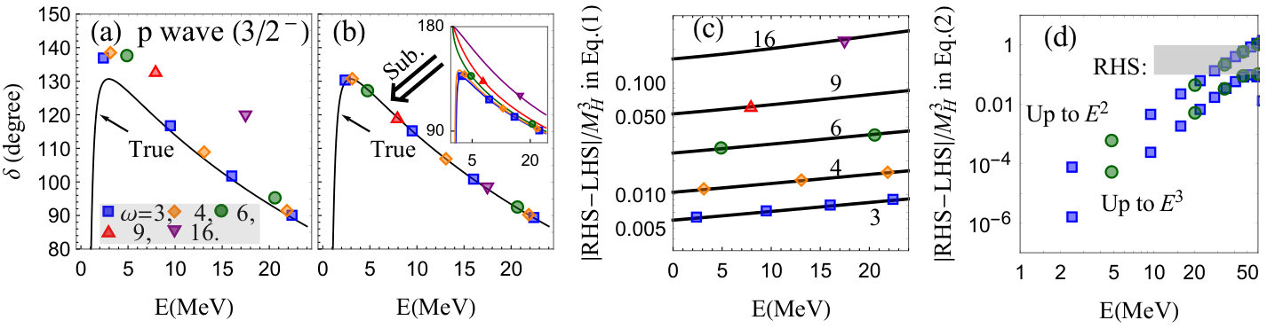 Figure 1
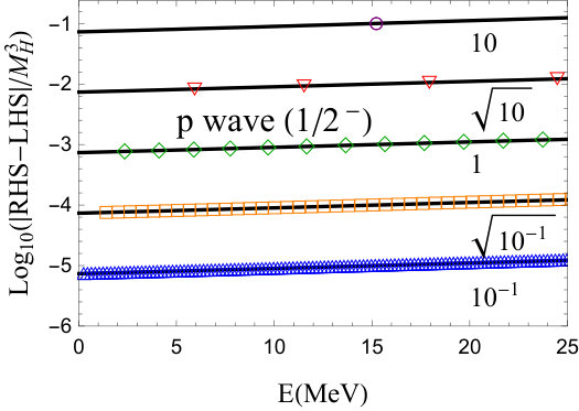 Figure 2
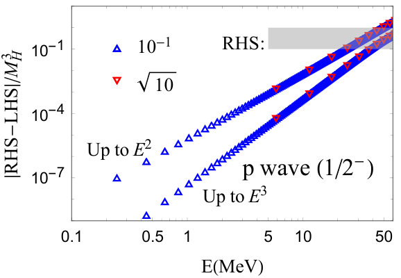 Figure 3
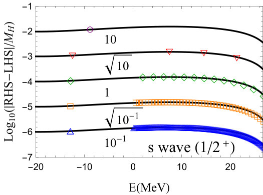 Figure 4
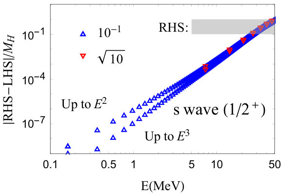 Figure 5
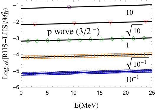 Figure 6
 Figure 7
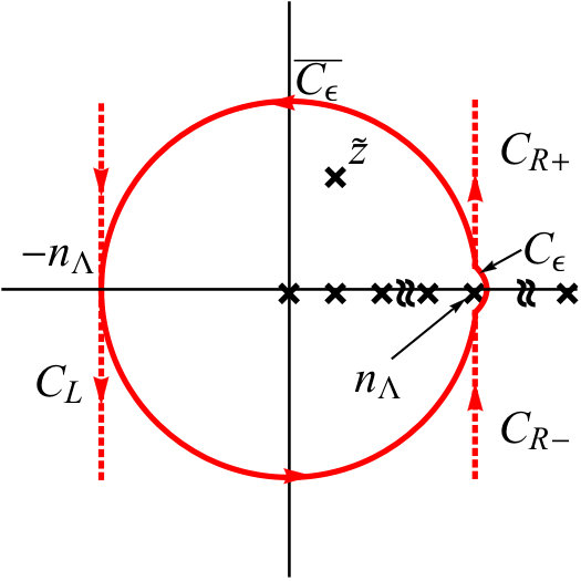 Figure 8
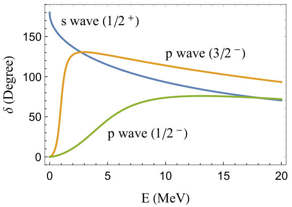 Figure 9
| 0.3536 | 0.4097 | 0.004206 | |
| 0.7898 | 0.1756 | 0.4063 | |
| 0.1743 | 0.2010 | ||
| 0.01278 | 0.2949 |
| 0.02304 | 1.870 | 0.5400 | |
| 0.5571 | 0.8676 | 0.3118 | |
| 0.5609 | 0.2829 | ||
| 0.08738 | 0.03911 |
| 0.1390 | 2.084 | 0.7400 | |
| 0.4427 | 1.090 | 0.5210 | |
| 0.6225 | 0.4064 | ||
| 0.1114 | 0.08700 |
Peer Reviews
No public reviews on file for this paper yet. If you reviewed it on a platform where reviews are public (OpenReview, ICLR, NeurIPS, ICML), you can paste yours below so the community can read it here.
Videos
No videos yet. Explain this paper in a talk, walkthrough, or lecture? Add one.
Extracting free-space observables from trapped interacting clusters
Xilin Zhang
Department of Physics, The Ohio State University, Columbus, Ohio 43210, USA
Physics Department, University of Washington, Seattle, WA 98195, USA
(April 28, 2020
)
Abstract
The energy spectrum of two short-range interacting particles in a harmonic potential trap has previously been related to free-space scattering phase shifts. But the existing formula for systems with a non-zero interaction range is exact only in the limit of an infinitely shallow trap. Here I provide a systematically improved formula—describing the low-energy dynamics—that enables the use of finite traps. This paves the way for extracting nuclear scattering phase shifts from ab initio nuclear many-body structure calculations, a long-sought goal in nuclear physics. The derivation establishes effective field theory as a powerful framework for studying the connection between structure information of a trapped system (with two or more sub-clusters) and continuum physics in the fields of both nuclear and condensed-matter physics.
Introduction
Nuclear experiments at low energy can not manipulate many-body systems to the extent possible in condensed-matter or cold-atom experiments. However, with progress in many-body methods Barbieri and Carbone (2017); Barrett et al. (2013); Carlson et al. (2015); Lee (2009); Stroberg et al. (2019) and increasing computing power (and quantum computers Preskill (2018)), one can start manipulating nuclear systems computationally. Here, I show how trapping two clusters at low energy in a harmonic potential well tells us about their free-space scattering through a formula connecting low-energy phase shifts with the confined spectrum. In this approach the trap compacts the system and reduces the required degrees of freedom enough to allow controlled ab initio calculations, as will be demonstrated elsewhere. (See e.g., Nollett et al. (2007); Navrátil et al. (2016); Elhatisari et al. (2015); Shirokov et al. (2018) for other ab initio approaches of computing light-nucleus scatterings.)
A formula for particles in a harmonic-potential trap was derived in Ref. Busch et al. (1998), and later generalized to include the full energy dependence of the phase-shift (besides the scattering length term in Busch et al. (1998)) and for partial waves beyond s-wave Blume and Greene (2002); Block and Holthaus (2002); Bolda et al. (2002); Idziaszek and Calarco (2006); Stetcu et al. (2007); Suzuki et al. (2009); Stetcu et al. (2010); Rotureau et al. (2010); Blume (2012). The result for angular momentum Suzuki et al. (2009); Stetcu et al. (2010); Luu et al. (2010) (called the BERW formula here) is
[TABLE]
This holds at the eigenenergies —with the center-of-mass (CM) energy subtracted—in a trap where each particle experiences a potential times its mass; is the reduced mass and the phase shift. Equation (1) is analogous to the Luscher formula Luscher (1991); Beane et al. (2004) that is widely applied in Lattice Quantum Chromodynamcs (for a system on a space-time torus).
Refs. Luu et al. (2010); Rotureau et al. (2012) have used Eq. (1) to extract nuclear scattering from ab initio spectrum calculations.
However, away from the infinitely-shallow-trap limit (i.e., for ), Eq. (1) does not capture the external potential’s modifications to the interaction at short distances. To illustrate the impact on extracting phase shifts, I use a two-body potential model Ali et al. (1985) designed for describing neutron- scattering [see the supplemental materials (SM) for details]. Figure 1(a) shows p-wave phase shifts extracted using Eq. (1) at the eigenenergies with MeV (typical values applicable in ab initio calculations): they fail to align on a smooth curve and systematically deviate from the exact curve Luu et al. (2010).
Here, I remedy the BERW formula using pionless effective field theory (EFT) van Kolck (1999); Bedaque and van Kolck (2002); Hammer et al. (2017), which enables low-energy dynamics to be studied without specifying the details of the short-distance physics (e.g., potential or cluster structure and excitation). This EFT was used to re-derive and generalize the Luscher formula Beane et al. (2004); Briceno et al. (2013). The improved formula for a harmonic trap is
[TABLE]
The constants depend implicitly on but are independent of and ; they are dimensionful and scale as proper powers of a high-momentum scale (as dictated by, e.g., the cluster excitations), unless there is fine tuning. When and are smaller than , the series sum converges and thus can be truncated with a controlled error. However, outside the convergence domain, where the details of the finite-range interaction and its interplay with the trap potential are being probed, the series expansion becomes infeasible. It is also worth noting that in the case of physically zero-range interactions (i.e., ), the terms, which capture the trap-induced modifications, would vanish, and Eq. (2) becomes equivalent to Eq. (1).
To infer the phase shifts from Eq. (2) given the eigenenergies, the terms must be simultaneously calibrated with the . The latter determine the free-space phase shifts via the effective range expansion (ERE) van Kolck (1999); Hammer et al. (2017). Knowing the full potential in the n- model, one can fix (see the SM) and generate Fig. 1(b): the inset shows that the phase shifts extracted from Eq. (1) for a given sit on a curve parameterized by a generalized ERE, in which the -order coefficient is given by . After subtracting the trap-induced modifications, the extracted phase shifts agree with the “True” curve.
The essence of Eq. (2), that the trap-induced modifications can be parameterized using a Taylor expansion in the and variables, can be seen in Fig. 1(c). The symbols show the differences between the right-hand-side (RHS) and left-hand-side (LHS) in Eq. (1)—scaled by —at the -dependent eigenenergies, while the solid lines plot the summation of the terms in Eq. (2)’s LHS with and . Indeed, they interpolate those symbols. Of course, outside the convergence domain, the series expansion would fail, as shown in Fig. 1(d). The differences between Eq. (2)’s two sides, based on two series truncations ( for “Up to ” and for “Up to ”, and in both cases), are plotted against a large range of eigenenergies. The truncation errors behave as the leading terms left out of the summation in the low-energy region, but then increase to when the symbols reach the shaded region indicating the range of Eq. (2)’s RHS; this also suggests the breakdown scale for is between and MeV. (See the SM for more details on series convergence.)
To extract nuclear phase shifts (or s) from ab initio spectra, Eq. (2) will play a crucial role, because ab initio calculations, developed to computing compact nuclei, have uncontrolled errors when . To illustrate Eq. (2), two models are used in the SM: a hard-sphere potential model is solved exactly, while the n- model is studied numerically. The rest of the paper is devoted to the derivation of Eq. (2), emphasizing a new set of interaction vertices between the external potential (or background field) and trapped particles, and renormalization.
Derivation through EFT
I start by constructing an EFT Lagrangian for two spin-[math] particles—for simplicity—in the partial wave, with a harmonic potential coupled to each particle. The framework is valid at low energies, where the details of the short-distance physics and its interplay with the trap are not resolved. I follow the conventions of Ref. Zhang et al. (2018). Let and be particle fields with masses and ( and are the complex conjugations), while is the so-called dimer field Kaplan et al. (1998a); Beane and Savage (2001); Bedaque and van Kolck (2002); Bedaque et al. (2003); Braaten and Hammer (2006); Briceno et al. (2013); Hammer et al. (2017) with spin , projection , and mass (). The dimer couples to - and represents the compound system. The background field is in the Lab frame with as a reference mass. The propagator—and the related self-energy corrections due to - multiple scattering—will be the central piece in the derivation: in free space it is directly related to the - scattering -matrix, while in the trap its poles give the system’s spectrum.
The Lagrangian is , where
[TABLE]
The building blocks of are invariant under Galilean transformations, including rotation, translation, and boost. (A relevant discussion on Galilean invariance in EFT can be found e.g., in Ref. Braaten (2015).) In both lagrangians for , , or , the structures with are ’s internal energies (i.e., total energies with kinetic and external potential energies subtracted), and therefore Galilean invariant.
The coupling in uses -’s relative velocity , while denotes a rank- operator composed of copies of normalized such that when , with . This term means is coupled to a - configuration having and as its relative angular quantum numbers. The indices are implicitly summed up so that this term is a scalar. (In general, the spin and vector indices need to be properly contracted to form scalars.) In addition, both and spins are invariant under translation and boost, and thus the coupling preserves Galilean invariance. Note that repeated indices in the Lagrangian (and in Eqs. (6), (8), and (9)) are implicitly summed with specified ranges.
It should be mentioned that the interactions in and with the external potential turned off follow closely previous works using a dimer-field approach Kaplan et al. (1998a); Beane and Savage (2001); Bedaque and van Kolck (2002); Bedaque et al. (2003); Braaten and Hammer (2006); Briceno et al. (2013); Hammer et al. (2017): (), , , and together reproduce the ERE (see Eq. (6) and Briceno et al. (2013); Beane and Savage (2001)). This approach is equivalent Kaplan et al. (1998a); Bedaque and van Kolck (2002); Braaten and Hammer (2006) to the EFTs without dimer fields (see further discussion in the “further comments” section).
The terms are also Galilean invariant, considering the external potential is a scalar field. However, their specific structures are severely constrained by a unique property of a harmonic potential: the CM of a multi-particle system is decoupled from its internal dynamics Caprio et al. (2012). (It can be understood based on that the external force on the multi-particle’s CM depends only on CM’s location in the harmonic potential well, i.e., not affected by any other degrees of freedom.) In these couplings with , ensures that they only shift the system’s energy by -independent but -dependent functions so that the CM behaves as a free particle in traps, i.e., decoupled from internal dynamics.
Besides powers of , the other possible scalar objects built of include (1) , , …(2) , , …[ is proportional to ], and (3) products of (1) and (2). (Derivatives higher than applied on would give zero, and therefore are not relevant here.) They would induce external potentials with powers of higher than 1. Copies of can also be used to construct tensor (vector) objects, which create anisotropic external potentials that need to be coupled to particles’ momenta or spins. As the result, the new scalar and tensor objects and their products would break the CM–internal-dynamics decoupling if they are present in any interaction terms with particles.
In principle, can be coupled to the operators (e.g., the term), which again must take the form of . However, these terms can be eliminated by rescaling the field by Coleman et al. (1969). Since the rescaling-induced terms are already present as couplings in , the trap modification to is not included.
Lastly in the free space, defining energy relative to the - threshold sets . Both are modified by through “polarization” effects as by couplings, but they only affect the energy-references in traps and for simplicity not shown here.
To compute the propagator of the dimer , its self-energy correction due to - multiple scattering needs to be included. A cut-off on momentum is applied to regularize loops in free space, while in traps the cut-off is applied on the virtual excitation energy van Kolck (1999). (However, for fine-tuned systems other schemes would be preferred, e.g., power divergence subtraction Kaplan et al. (1998b).) Within time-independent perturbation theory Zhang et al. (2018), the one-loop self-energy bubble diagram in free space is . and are the Hamiltonians derived from and the term in , respectively Zhang et al. (2018). Both states are plane waves, with , , , , and as ’s momenta and energy in the Lab frame, and its spin projections. (The realtionships between Feynman diagrams and the matrix elements defined here and below can be found in Ref. Zhang et al. (2018).) One then obtain
[TABLE]
, , is the cut-off on , and . is the energy in the CM frame. Note as .
The fully dressed free-space propagator, which is defined through , with from , can be computed by summing the self-energy-insertion diagrams due to and the vertices, yielding
[TABLE]
is related to through the scattering -matrix, which is computed by multiplying with two -vertices Zhang et al. (2018). The range of the index in in the implicit sum is fixed in , and in the definition is the component of the list and is not summed.
Now let us turn to the trapped system. Based on , one can expand , and fields using their corresponding harmonic-oscillator wave functions Stetcu et al. (2010). Again note that the coupling only picks up the - configuration whose total angular momentum and projection equal those of the CM motion (i.e., ) and whose relative angular momentum and projection equal the ’s spin and projection ( and ). Thus the matrix element between ’s eigenstates in a trap for defining its self-energy becomes (note the absence of in the Green’s function), with
[TABLE]
Here and the relative energy , with as the CM’s energy. If and receive trap-dependent “polarization” corrections, these corrections also need to be subtracted in defining . In the derivation, a unitary transformation between and single-particle and CM/relative motion eigenmodes has been used.
Summing over the quantum numbers associated with the intermediate state’s CM motion gives rise to the factor in defining , since the CM’s decoupling property is preserved and thus so is . For the relative dynamics, is part of the eigenmode function Stetcu et al. (2010): . has for its radial excitation and angular momentum, and . A cut-off on is used to regularize the theory in a trap, which is in parallel with the regularization used in Eq. (5).
The propagator in the trap, defined as , can be computed by summing up all self-energy insertion diagrams, including insertions of and those of the and vertices. One get
[TABLE]
In the 2nd step, the principal value of the free-space self-energy is added and subtracted. Thus, the quantization condition can be derived by setting the denominator in Eq. (8) to zero:
[TABLE]
There exists a special relation between (or ) and such that the divergences in and cancel in Eq. (9), and thus are finite. For s-wave, , but for p-wave the -order term needs to be specified: ; for d-wave another higher order term needs to be specified: ; for even larger , more terms need to be specified accordingly. Details on the renormalization can be found in the SM. However, the above - relations should be considered as a specific scheme; any alternative ones would need to ensure that the divergences in Eq. (9)’s right side can be absorbed by the terms in the left side so that phase shifts are cut-off independent and the CM-decoupling property is not violated.
The right side of Eq. (9) in this scheme then becomes
[TABLE]
with “” labeling the renormalized series sum with . To finish the derivation, this identity is needed:
[TABLE]
which holds in the entire complex plane (both sides have the same poles and residues, see the proof in the SM). By redefining in Eq. (9) and applying Eq. (11) in Eq. (10), Eq. (9) gives Eq. (2).
Further comments
It is worth comparing in Eq. (6) and in Eq. (8) in the complex plane. has a branch cut—known as the unitary cut—on the positive real axis due to the term, which changes into a series of poles—called “unitary” poles below—for (from the term ). Both non-analyticities are directly connected to unitarity and thus independent of framework, power counting, and fine tuning.
However, fine tuning and power counting do impact the behavior of the ERE function van Kolck (1999): in a natural case, ; in a fine-tuned case, is enhanced; and in a fine-tuned case, the function has low-energy poles. Note Ref. van Kolck (1999) uses EFTs without a dimer field; and the Lagrangian is the same for the three cases, except power countings. One can add the couplings between and particles to the Lagrangian, again by multiplying the short-distance-interaction terms with powers of , e.g., for s-wave .
For each of these cases, the -Matrix in a trap can be computed in the same way as the free-space one van Kolck (1999) but with the bare couplings substituted by the corresponding modified ones—e.g., —and the unitary cut by the “unitary” poles. Since the EFT calculations reproduce the free-space -matrix using ERE parameters , the -matrix in a trap can be parameterized in the same way but with -dependent ERE parameters. The relation between these ERE parameters and the bare couplings is nonlinear, but the former’s -dependence could be expanded in terms of . (This expansion must be examined with care, if its convergence radius is much smaller than the naive estimate based on , e.g., due to fine-tuning of the trap’s modification to the interaction at short distance.) Finally, by identifying the poles of the trap -Matrix, one then reproduces Eq. (2) for the natural and the fine-tuned case; for the fine-tuned case, a Laurent expansion of was derived van Kolck (1999), so the same expansion should be used in Eq. (2)’s left side with the parameters carrying corrections. In other words in my approach with a dimer field, resumming of and terms is needed.
Summary
I have applied pionless EFT to two short-range interacting particles in an external harmonic trap to derive a systematically improved BERW formula that is exact even at finite . It is valid when the infrared scale of the trap () and the relative momentum () are both smaller than the high momentum scale set by the dynamics. This provides a firm foundation for implementing a Luscher-formula-like approach to connect nuclear scattering and ab initio structure calculations. The derivation involved new coupling terms between the background field and particles, which lead to the improvements of the original BERW formula. Moreover, a careful analysis of renormalization shows a non-trivial relation between the cut-off on relative momentum in free space and cut-off on the number of radial excitation in a trap. The renormalization procedure is further confirmed by Eq. (11)’s proof. Both aspects are instructive for deducing connections between a trapped system (with two or more clusters) and free-space scattering/reactions for both nuclear and cold atom physics Blume (2012). It should also be interesting to apply this framework to study exotic atoms111Here the long-range interaction is the attractive Coulomb force. The so-called Deser–Trueman formula Combescure et al. (2007) relates exotic atom’s energy levels to the short-distance interaction’s scattering length. and quantum dots Combescure et al. (2007).
Acknowledgment
I would like to thank Dick Furnstahl, Chan Gwak, Jason Holt, David Kaplan, Ubirajara Van Kolck, Petr Navratil, Daniel Phillips, Martin Savage, Ragnar Stroberg, and Chieh-Jen Yang for helpful discussions, and Yuri Kovchegov for pointing out how to use contour integration to prove Eq. (11). I also thank Dick Furnstahl and Jordan Melendez for careful proofreading of the manuscript. The work was supported by the National Science Foundation under Grant No. PHY–1614460 and the NUCLEI SciDAC Collaboration under US Department of Energy MSU subcontract RC107839-OSU, the US Department of Energy under contract DE-FG02-97ER-41014, and the US Institute for Nuclear Theory.
I An exactly solvable case: hard-sphere potential
I demonstrate here that if the interaction is short-ranged and has the form of a hard sphere, the parameters in the improved BERW formula (i.e., Eq. (2) in the main text) can be found analytically. This model was studied in Ref. Block and Holthaus (2002) by using parabolic cylinder functions for s-wave channel. The hard-sphere potential is defined as if and [math] otherwise ( with the relative displacement between the two particles). In addition, each particle experiences an external harmonic potential. Because the CM motion is factorized, one can just focus on the relative motion; the corresponding external potential is , with the reduced mass.
Let us define and with , and . When , the Schrödinger equation in the partial wave becomes
[TABLE]
with the radial wave function defined as . Thus, the wave function at is a linear combination of two independent solutions to the harmonic oscillator Schrödinger equation Suzuki et al. (2009):
[TABLE]
where is the Kummer function Abramowitz and Stegun (1972).
When , should go to zero to guarantee that the wave function is normalizable. Since at large (DLMF, , Eq. 13.7.2)
[TABLE]
the following is required:
[TABLE]
Meanwhile, implies
[TABLE]
Equations (S4)–(S5) have nontrivial solutions only if the corresponding determinant is zero, which gives the quantization condition:
[TABLE]
Here, [].
Note that the left side of Eq. (S6) is the right side of the main text’s Eq. (1) multiplied by a factor. Meanwhile, the phase shift due to in the partial wave is Joachain (1975). Thus the discrepancy of the BERW formula is identified as the difference between the left side of the main text’s Eq. (1) multiplied by and the right side of Eq. (S6), i.e.,
[TABLE]
The left side can be expanded in terms of :
[TABLE]
Now according to Ref. (DLMF, , Eq.(13.2.2)), can be expanded as , indicating that Eq. (S7)’s right side, a function of and , can be approximated by a double expansion in terms of powers of and when both are small (note that the coefficient denominators in the expansion of the functions in Eq. (S7) are independent of and ). This also suggests the difference between left and right sides in Eq. (S7) can be expanded in terms of and .
It can be shown that with and and fixed, the right side of Eq. (S7) approaches its left side. In this limit, ,
[TABLE]
where is a Confluent Hypergeometric Limit Function. Reference Petkovšek et al. (1996) suggests
[TABLE]
Since
[TABLE]
one then obtain
[TABLE]
and thus prove that the difference between the two sides of Eq. (S7) disappears as . This requires that the difference, if expanded in terms of and , must have positive powers of ().
Moreover, both sides of Eq. (S7) are unchanged when and (i.e., ), because (DLMF, , Eq.(13.2.39)), indicating that the powers of are positive and even (the powers of are non-negative integers). Therefore, the following expansion is expected, with the first two terms explicitly given:
[TABLE]
Meanwhile, the ERE for can be derived easily from Eq. (S8): . If a high-momentum scale is identified, Eq. (S14) can be transformed to the improved BERW formula after redefining .
II The 2nd model for numerical testing
In contrast to the analytical study in the last section, here a simple square-well model Ali et al. (1985) is used to numerically demonstrate that the discrepancy of the BERW formula can be expanded in terms of powers of and , which is the essence of the improved BERW formula. The potential was constructed to qualitatively describe neutron- scattering in the s- and p-waves Ali et al. (1985). The quantum numbers for the considered channels in notation are , and . The potential when and [math] when , with MeV, fm, Ali et al. (1985). is the spin-orbit coupling, which generates differences between the and channels.
In this exercise, the potential is treated as the exact underlying physics for the two particles. The phase shifts, calculated by solving the corresponding Schrödinger equations in the continuum, are shown in Fig. S1. These phase shifts are considered to be “exact” ones. (The channel’s exact phase shift is also shown in Fig. 1 in the main text.) Meanwhile, the spectra for the two particles in various harmonic potential traps can also be precisely computed. The goal is to test the original and the improved BERW formulas using these exact phase shifts and energy spectra.
In Fig. S2, the discrete symbols are the differences between the two sides in the main text’s Eq. (1) divided by at eigenenergies associated with the trap frequency , , , and MeV. Here, I take MeV (), as motivated by the value of . One can see that the leading-order difference does scale as . Also, in the s-wave channel there is a deep bound state in free space—unphysical for the n- system—and thus a distinct negative eigenenergy in all the traps. However, for the other two channels no bound state exists in free space.
To see how well the improved BERW formula works, one need to know the values of corresponding to this particular potential. First, another set of eigenenergies at extremely small trap frequencies (both on the order of MeV) is computed. Second, they are used as inputs to fit values based on the improved BERW formula. A least-squares fit uses as the objective function the sum of the squares of the differences between the two sides in the improved BERW formula, as calculated at those small eigenenergies. The small values of and eigenenergies help separate the impact of at different orders, and enables a precise fit (it amounts to computing derivatives at and with points separated by tiny distances). The series in the improved BERW formula is nonetheless truncated to and . To make the parameters dimensionless, one can rescale them by appropriate powers of , . The best-fit values for are shown in Tables 1, 2, and 3.
A few higher-order values are not shown in those tables, because over-fitting Furnstahl et al. (2015) in this simple exercise leads to values significantly larger than . However, these contributions are very small in the plots shown if they on the order of (their natural size), and therefore they are set to zero in generating the plots.
Having determined the , the terms in the improved BERW formula are used in Fig. S2 to interpolate between the discrete symbols, i.e., the difference between the right and left sides of the BERW formula as computed at discrete eigenenergies up to MeV. Because the fitting of is carried for and near zero ( MeV), the agreement with the interpolating curves and discrete symbols demonstrates that the discrepancy of the BERW formula can indeed be expanded in terms of powers of and , as implied by the improved BERW formula.
However, the truncation on the series sum in the improved BERW formula inevitably leads to truncation error. Fig. S3 plots such errors, i.e., the difference between the formula’s two sides with the index summed up to either (for the “Up to ” results) or (for the “Up to ” results) and with index summed up to for both cases. The shaded region shows the rough range of the formula’s RHS with above 5 MeV. In the low energy region, the error does behave like the leading terms left out of the series sum, but it increases with and eventually reaches the shaded region. The latter signals the break down of the series expansion, as the error reaches . This also suggests the break down scale for is above MeV and perhaps below 40 MeV in all three channels, which are consistent with my choice of MeV. Note the behavior of the error above the break down scale could be more complicated than the simple power law in the low-energy region. In fact in all these channels, the errors oscillate and change their signs in the higher-energy range not shown in the plots.
III Details on the renormalization in the EFT derivation
This section discusses the particular renormalization scheme mentioned in the main text, in which the divergences in in and cancel in Eq. (9) in the main text. This scheme gives a specific relation between and . To derive this relation, the -dependence of needs to be studied.
Two formulas are useful for understanding at large and at large . The first is (DLMF, , Eq. 5.11.13)
[TABLE]
Here and are real or complex constants, and as a function of and is related to the generalized Bernoulli polynomials (DLMF, , Eq. 5.11.17) Temme (1996). The second is the Euler–-Maclaurin formula (DLMF, , Eq. 2.10.1), stating that for a smooth , its series sum can be approximated using an asymptotic expansion:
[TABLE]
where is a Bernoulli number. Only the dependent terms are shown. Like , the to derivatives of diverge. So for s-waves, only is considered:
[TABLE]
Thus () so that the divergence can be absorbed by in the main text’s Eq. (10). The term in the - relation is not relevant when . For p-waves, the and first derivatives are divergent:
[TABLE]
Thus, , to have these divergences canceled by those in in the main text’s Eq. (10). The piece in the expression must be specified, but higher-order terms are not needed. However for d-waves, another order higher needs to be specified: ; for even larger , more terms need to be specified accordingly.
This requirement is tied to the fact that for a specific -derivative, there is a tower of divergences with different degrees in (e.g., Eq. (S18)), in stark contrast with the same derivative of , where the power of is fixed by the the dimensions.
IV A proof of Eq. (11) in the main text
Let us redefine , and
[TABLE]
The main text’s Eq. (11) then becomes
[TABLE]
The renormalization is defined by Eq. (10) in the main text and the relationship between and that guarantees the cancellation of the divergences on that equation’s left side. The proof starts with integrating in the complex plane over a large contour around the origin and crossing between the two singularities at and on the positive real axis. The contour is plotted in Fig. S4. After rearranging terms one get
[TABLE]
The left side comes from the residue of the pole in the contour integration while the series sum on the right side is from the residues of ’s poles (all on the positive real axis) in the same integration. Comparing Eq. (S23) to Eq. (S22) suggests that the contour integration in Eq. (S23) should cancel the series’s divergence as the terms—i.e., those from —do in the main text’s Eq. (10). This is the focus of the following proof.
As preparation, it is important to understand the behavior of in two different regions (define and as the radius of ): and . Let us look at the region close to the positive real axis first. Considering the presence of ’s poles, it is easier to use the following re-expression based on (DLMF, , Eq. 5.5.3):
[TABLE]
This expression moves the poles from the function to the function. When ,
[TABLE]
Here is a small positive number. Therefore, when [the error scales as ], but in the region, , and its behavior is qualitatively different.
Since the function ratio in Eq. (S24) is the same as that ratio in with , by applying the asymptotic expansion from the main text’s Eq. (11) on the right side of Eq. (S24), I get, when such that and when ,
[TABLE]
Here is the asymptotic expansion of in terms of using the main text’s Eq. (11). It turns out the above expansion also holds when or . However, using Eq. (S24) to understand close to the negative real axis is awkward, as it involves the cancellation of poles from the and the functions. Instead, Eq. (11) in the main text can be applied to analyze the original form of (see Eq. (S21)):
[TABLE]
Here is used, which can be inferred from its definition (DLMF, , Eq. 5.11.17) Temme (1996) and properties of the generalized Bernoulli polynomials. It is worth pointing out that the factor moves the asymptotic series’s branch cut on the negative real axis due to the 222As usual (DLMF, , Eq. 1.9.7), the branch cut in the complex plane is on the negative real axis. Meanwhile (and the related scattering -matrix), as calculated in the main text’s Eq. (5), in the complex plane has a branch cut separating physical and unphysical sheets on the positive real axis Goldberger and Watson (1964), because it involves . factor to the positive real axis, ensuring that the expansion series is analytic around the negative real axis. Therefore, Eq. (S26) holds when , but not in the region. This suggests splitting the contour integration into two major pieces:
[TABLE]
In , is the point where crosses the real axis. Thus the contour means to integrate infinitely close to the upper and lower real axis, because of the corresponding integrand’s branch cut on the positive real axis. In the piece, the first term should be integrated over . However, since the integrand is continuous across the point as long as , changing the contour to does not affect the results.
Integrating the piece over with gives
[TABLE]
Here truncates the expansion in by only keeping terms with powers of from to (the neglected terms’ integration vanishes no slower than as ). In the derivation, (1) the branch has been rotated by , which eliminated the factor because of the factor in the integrand; (2) a transformation, , was used; and (3) the fact that is analytic in the upper complex plane and an even function on the real axis was used. Note that integrating the piece over gives [math] with .
For the piece, the contour can be deformed to without crossing any singularities, with the left and right segments connecting at . The integrand on the two sets of contours (including in the area enclosed by them) is 0 up to at most a correction (with as a positive number), except on the segments with along and . Therefore, can be safely ignored. Let us focus on . Since
[TABLE]
the piece is
[TABLE]
Note that when , its integration over with gives .
Integrating over with gives
[TABLE]
Because the integration is dominated by the region, the two are expanded in terms of Taylor series for the argument at in the above derivation. The resulted integrations are proportional to Riemann at even arguments, which are related to Bernoulli numbers (DLMF, , Eq. 25.5.1, 25.6.2, 24.2.2). Adding all the contributions, one can see that the term on the right side of Eq. (S23) can be approximated by
[TABLE]
with the leading error scaling as [see the discussion of . In comparison, the error ( is a positive constant) is much smaller with large ]. The above expression is exactly the same as the divergent -dependent pieces in ’s series sum derived using Eq. (S16) in the previous section, which completes the proof.
The reference list from the paper itself. Each links out to its DOI / PubMed record.
- 1Barbieri and Carbone (2017) C. Barbieri and A. Carbone, Lect. Notes Phys. 936 , 571 (2017) , ar Xiv:1611.03923 [nucl-th] . · doi ↗
- 2Barrett et al. (2013) B. R. Barrett, P. Navratil, and J. P. Vary, Prog. Part. Nucl. Phys. 69 , 131 (2013) . · doi ↗
- 3Carlson et al. (2015) J. Carlson, S. Gandolfi, F. Pederiva, S. C. Pieper, R. Schiavilla, K. E. Schmidt, and R. B. Wiringa, Rev. Mod. Phys. 87 , 1067 (2015) , ar Xiv:1412.3081 [nucl-th] . · doi ↗
- 4Lee (2009) D. Lee, Prog. Part. Nucl. Phys. 63 , 117 (2009) , ar Xiv:0804.3501 [nucl-th] . · doi ↗
- 5Stroberg et al. (2019) S. R. Stroberg, S. K. Bogner, H. Hergert, and J. D. Holt, Ann. Rev. Nucl. Part. Sci. 69 , 307 (2019) , ar Xiv:1902.06154 [nucl-th] . · doi ↗
- 6Preskill (2018) J. Preskill, ar Xiv e-prints , ar Xiv:1801.00862 (2018), ar Xiv:1801.00862 [quant-ph] .
- 7Nollett et al. (2007) K. M. Nollett, S. C. Pieper, R. B. Wiringa, J. Carlson, and G. M. Hale, Phys. Rev. Lett. 99 , 022502 (2007) , ar Xiv:nucl-th/0612035 [nucl-th] . · doi ↗
- 8Navrátil et al. (2016) P. Navrátil, S. Quaglioni, G. Hupin, C. Romero-Redondo, and A. Calci, Phys. Scripta 91 , 053002 (2016) , ar Xiv:1601.03765 [nucl-th] . · doi ↗