Perturbations to Generalized Kink-like Topological Defects in $AdS$
Orlando Alvarez, Matthew Haddad

TL;DR
This paper investigates the stability of perturbations to kink-like topological defects in anti-de Sitter spaces, extending previous work to higher dimensions and demonstrating stability of scalar field perturbations.
Contribution
It generalizes earlier results by analyzing perturbations in higher-dimensional $AdS$ embeddings and shows their stability at first order.
Findings
All perturbations to the scalar field mass are stable to first order.
The equation of motion for perturbations resembles a well-known quantum mechanics problem.
Extended analysis from $AdS_2$ to higher-dimensional $AdS$ spaces.
Abstract
We explore perturbations to a kink-like (codimension 1) topological defect whose world brane is embedded into . Previously, we found solutions in the limit the mass of the scalar field vanishes. In this article we extend a calculation previously done in to higher-dimensional embedding spaces and find that all perturbations to the mass of the field are stable to first order as expected in a theory with topological defects. We find that the equation of motion to the correction strongly resembles a problem well-known in quantum mechanics.
Click any figure to enlarge with its caption.
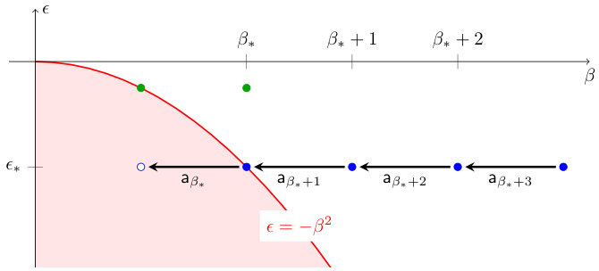 Figure 1
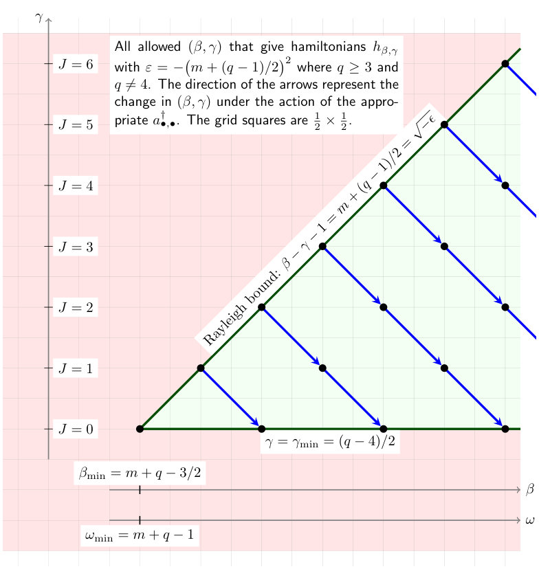 Figure 2
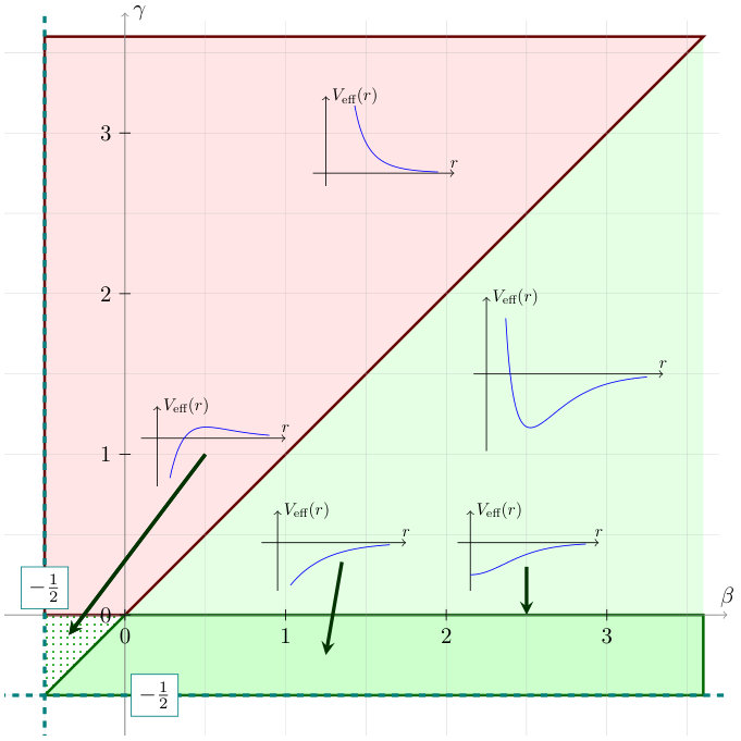 Figure 3
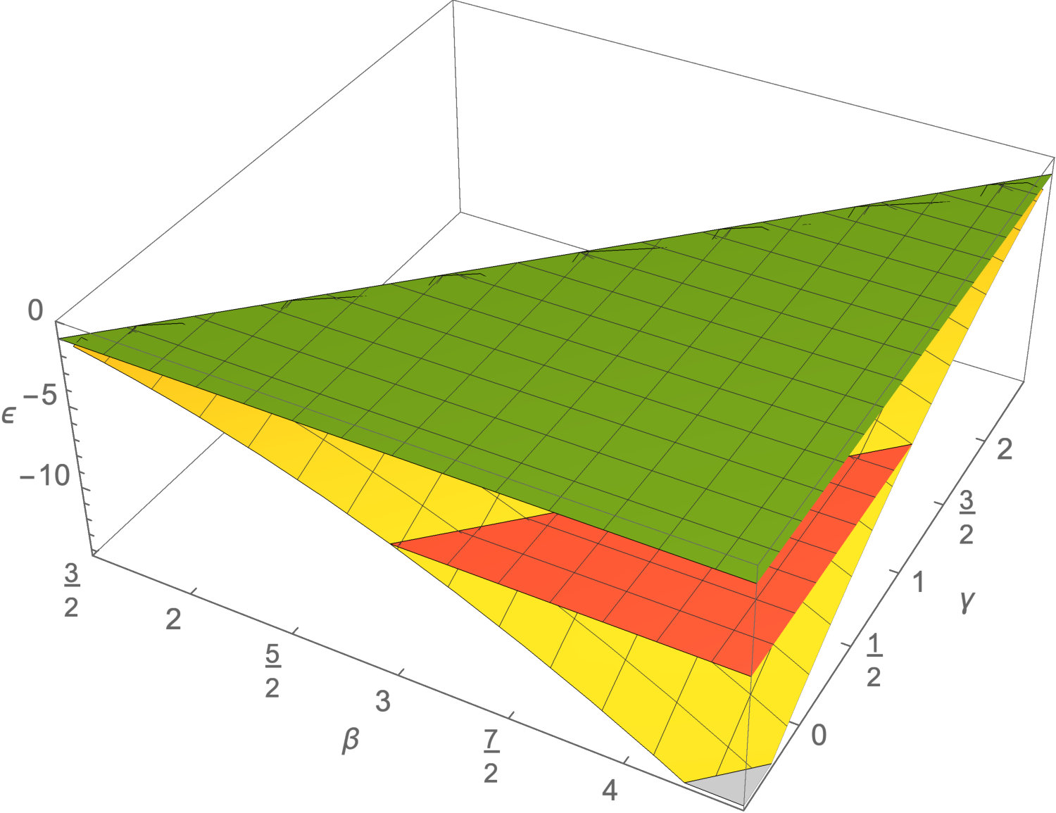 Figure 4
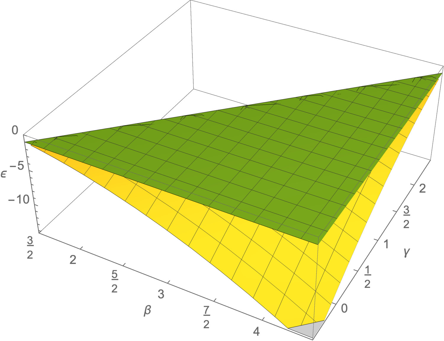 Figure 5
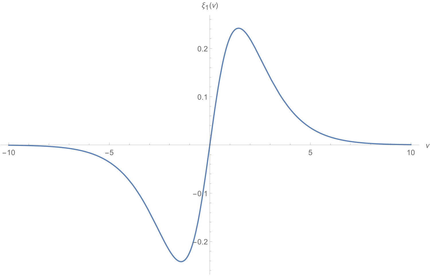 Figure 6
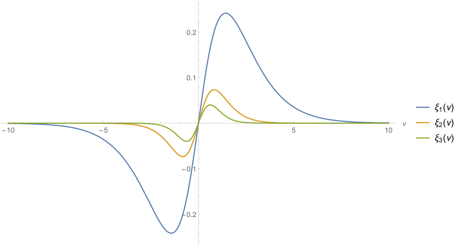 Figure 7
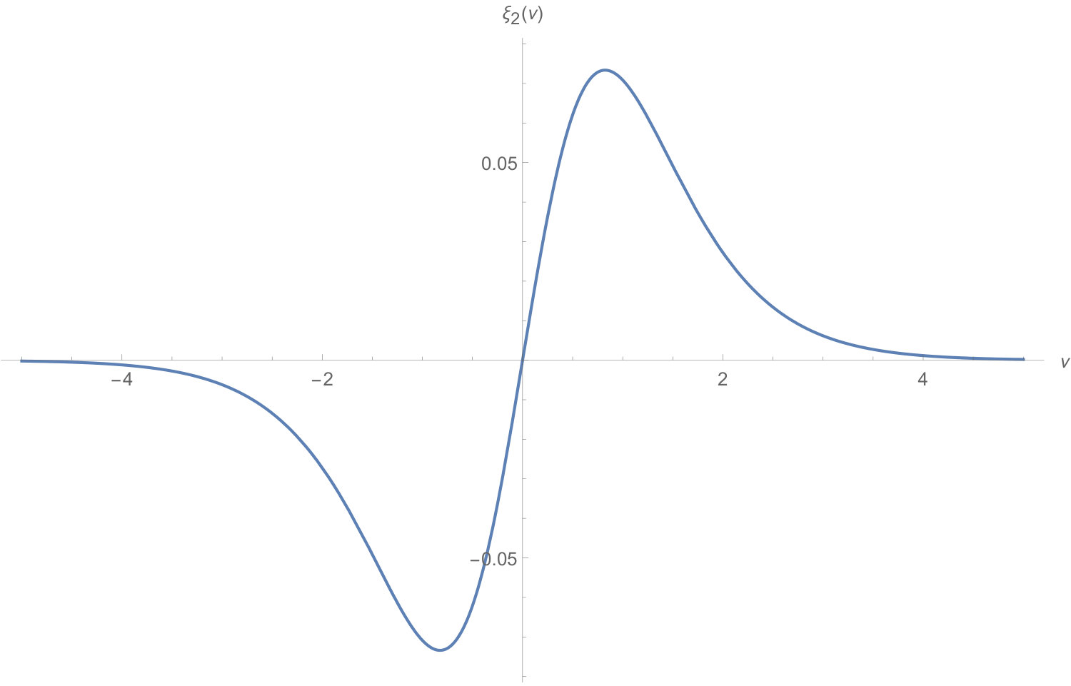 Figure 8
 Figure 9
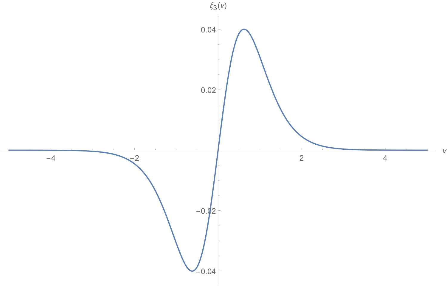 Figure 10
Peer Reviews
No public reviews on file for this paper yet. If you reviewed it on a platform where reviews are public (OpenReview, ICLR, NeurIPS, ICML), you can paste yours below so the community can read it here.
Videos
No videos yet. Explain this paper in a talk, walkthrough, or lecture? Add one.
\mmddyyyydate
Perturbations to Generalized Kink-like Topological Defects in
Orlando [email protected]
Department of Physics, University of Miami, 1320 Campo Sano Ave, Coral Gables, FL 33146
Matthew [email protected]
Department of Physics, University of Miami, 1320 Campo Sano Ave, Coral Gables, FL 33146
(Last Typeset: at \currenttime)
Abstract
We explore perturbations to a kink-like (codimension 1) topological defect whose world brane is embedded into . Previously, we found solutions in the limit the mass of the scalar field vanishes. In this article we extend a calculation previously done in to higher-dimensional embedding spaces and find that all perturbations to the mass of the field are stable to first order as expected in a theory with topological defects. We find that the equation of motion to the correction strongly resembles a problem well-known in quantum mechanics.
1 Introduction
This is the third of a series of articles in which the authors explore the dynamics of topological defects in anti de Sitter space. These objects are interesting to study as a possible consequence of symmetry breaking in the early universe leading to cosmological-scale objects such as cosmic strings [1]. In more recent years, some study has gone into how these objects might influence the dynamics of nearby massive objects [2] Our model concerns an -gauged Higgs-type field theory embedded into with . For convenience, we will often refer to these with the shorthand “ defect” for the codimension- topological defect with a worldbrane of embedded in . In the first article [3], we laid out a framework for finding exact analytical spherically-symmetric topological defect solutions. The method followed in the spirit of Bogomolny, Prasad, and Sommerfield (BPS) [4, 5], who were able to study exact solutions to the ’tHooft-Polyakov Monopole and Julia-Zee dyon in flat spacetime. The solutions we found were affectionately dubbed the “double BPS” solutions for that reason. In the double BPS solution, the finite radius of curvature of sets the length-scale for the physics, allowing one to take the limit in the equations of motion that the mass of the fields fall to zero. Lugo et al. [6, 7] and Ivanova et al. [8, 9] also did studies of topological defects in , especially that of monopoles in the former and pure Yang Mills solutions in the latter. For a discussion on how these works relate to this model and more detail on the process, we refer the reader to the original article [3].
The second article [10] concerned an extension of this using perturbation theory. Given a double BPS solution, we allow a small perturbation in the potential to reintroduce the mass of the field. We took the case of the (1,1) kink-like defect in particular; that is, the codimension-1 topological defect with a worldbrane that is embedded in . We found that these defects are stable under this perturbation and we were able to calculate the correction to the defect energy that results.
In this paper, we extend our discussion to a more general defect. We are able to show that these solutions are linearly stable in general as expected in a theory containing topological defects.
2 The metric and full EOM
The kink is a codimension-1 topological defect extending from a totally geodesic embedded in . There is still only a scalar field , so we do not have a gauge field to worry about. We take the metric of to be the standard maximally invariant Lorentzian metric333We use the mostly convention for the signature. on , with as coordinates along the submanifold. If is the sectional curvature of (and by extension, the totally geodesic ), then the radius of curvature is defined by . A point in will be given coordinates where is the signed distance along a geodesic that is normal to . Note that . The metric in is then
[TABLE]
From this point forward we will use dimensionless coordinates. These can be obtained by scaling everything by the radius of curvature: , , and where the vacuum expectation value for the scalar field .
The action for a -defect is
[TABLE]
where is a bookkeeping parameter that will be used to keep track of the order of the perturbative expansion. We assume the potential is of the symmetry breaking type with minimum at after the field rescaling.
This gives rise to the equation of motion:
[TABLE]
The first term is the negative of the d’Alembertian and which in our chosen coordinates may be expressed as :
[TABLE]
Using this operator, equation (2.3) becomes:
[TABLE]
This is the wave equation with a source. In the limit where , we obtain the wave equation . In addition, we retain the boundary conditions
[TABLE]
that guarantee a kink-like solution. We seek solutions with localized energy, that is, energy density that falls off exponentially as . It does not need to be localized in the direction(s).
We found maximally symmetric solutions that depend only on the normal coordinate , and we denoted them by . These are the so-called double BPS solutions and they satisfy the wave equation
[TABLE]
with boundary conditions as , and is discussed in [3]. We are interested in analyzing the corrections to our solutions by introducing a perturbation about the double BPS solution, and we write the field as the double BPS solution and a perturbation: .
The first-order correction obeys a wave equation with a source term determined by the zeroth order double BPS solution:
[TABLE]
The general solution will consist of a particular solution to the inhomogeneous equation and the general solution to the homogeneous equation: , where solves the inhomogeneous equation with a source and solves the homogeneous equation. Our ansatz for the perturbative solution is therefore .
This was only to first order, but it’s not too hard to generalize this procedure to any order in perturbation theory. We can show that, in general:
[TABLE]
where we use to denote the th order solution to the equations of motion. This gives an iterative scheme to solving the differential equation. At each order you will have to specify exactly how to choose the solution to the inhomogeneous equation because the d’Alembertian operator has a non-trivial kernel. To uniquely specify a perturbative solution we use the same method as in the case.
3 Solving the EOM
3.1 Separating the EOM
The first order contribution must satisfy (2.8). Since the source term on the right is only a function of , we can write , where is a particular solution to the inhomogeneous equation and is a solution to the homogeneous equation below:
[TABLE]
[TABLE]
The boundary conditions are and . Equation (3.1) is an ordinary linear differential equation with source and we immediately discuss its solution. Afterwards, we will discuss how to solve PDE (3.2),
3.2 Solving for
The solution to (3.1) depends upon the choice of potential . The solution in the case of the defect in the symmetry-breaking potential was explored in our previous article [10]. We restate the results here, and extend the discussion of this toy model to a few other cases. The procedure for solving the equation is nearly identical for , though the difficulty in obtaining the solution varies significantly as increases, see Appendix C for details.
In the case of , the ODE becomes:
[TABLE]
Here, is the squared flat-space mass of the scalar field scaled by the radius of curvature in order to keep dimensionless coordinates. The solution to this equation with the given boundary conditions is
[TABLE]
where is the polylogarithm function of order , and gd is the Gudermannian function.
When the ODE is given in (C.1). The solution to this equation with the appropriate boundary conditions is
[TABLE]
Though not immediately obvious, is real-valued, see Appendix C. We also obtained an explicit expression for the case . This expression is lengthy and does not appear to yield novel information. It is included for completeness in the aforementioned appendix. These solutions are plotted in figure 1.
3.3 Solving the equation for
We focus on solving the PDE (3.2) for . We use the separation of variables method and try a separable solution . Substituting into the equation, we obtain
[TABLE]
The first term involves only -derivatives and the second only involves -derivatives. Since these are independent, the only way they can cancel exactly is if they are equal to some constant . The first term gives:
[TABLE]
The second term gives:
[TABLE]
which can be rewritten as
[TABLE]
This is a one-dimensional problem. There is a gauge transformation we can do to eliminate the first derivative term and turn this equation into a Pöschl-Teller model in Schrödinger form.
3.4 The Pöschl-Teller model and the equation for
Consider the first order differential operator
[TABLE]
Squaring this operator leads to
[TABLE]
We can see that the first two terms are exactly the operator we have in (3.9), and with a little bit of algebra and hyperbolic function identities we can rewrite (3.9) as
[TABLE]
The covariant derivative like operator can be turned into an ordinary derivative via a gauge transformation. We note that
[TABLE]
and
[TABLE]
If we define the auxiliary function then we have
[TABLE]
Substituting (3.15) into (3.12) gives
[TABLE]
This is a Schrödinger-type differential equation with a Pöschl-Teller-style potential
[TABLE]
with eigenvalue of . The strategy is to determine all values of the parameter that lead to an eigenvalue . We work out the solution to this problem in Appendix A.1. For brevity, the normalized solution found there is:
[TABLE]
where , and is the rising factorial of . The values of that lead to an eigenvalue of for (3.16) are the infinite sequence
[TABLE]
We note that a consequence of and is that .
3.5 The Eigenvalue Problem for
Next we study equation (3.7) incorporating the correct expression for the eigenvalues (3.19). The equation for to be solved is
[TABLE]
This is the massive Klein-Gordon equation on the submanifold with mass that depends on the dimension and the index . We can work out the explicit form of . First, write the metric for as
[TABLE]
In these coordinates, we have split into the coordinates , and angles on . The metric determinant is therefore
[TABLE]
and (3.20) becomes
[TABLE]
The metric is diagonal, so we try separation of variables with ansatz
[TABLE]
where is the radial wave function, and are orthonormal real spherical harmonics on . Here is the angular momentum that labels the irreducible representation of . The index takes
[TABLE]
different values. Note that for , the formula above gives , which is the dimensionality of the real irreducible representations of .
For now, we will suppress the indices. If we plug this back in and divide the whole equation by per the usual procedure in separation of variables, we wind up with the equation:
[TABLE]
where is an eigenvalue of the Laplacian on . Note that the ODE is parametrized by , , , . We ignore because it is fixed, and this is why we had previously written .
We have managed to reduce our problem to an ODE in . Since this is a 1D problem, let’s try a gauge transformation (as we did prior) to see if we can eliminate the first derivative terms:
[TABLE]
The term inside the large parentheses is
[TABLE]
Putting all this together, we have
[TABLE]
We can use this to rewrite (3.25) as
[TABLE]
To eliminate the covariant derivative, let , then . If we also set then we can rewrite (3.30) as
[TABLE]
It should be mentioned that the Hilbert space that belongs to is plain old square integrable functions on . The reason is that is just the volume element factor (3.22) that enters the inner product required for the function . We next substitute the basic parameters into the above and algebraically simplify to obtain
[TABLE]
This is a Schrödinger-type equation with a generalized Pöschl-Teller type potential. We examine how to analyze the spectrum for this type of problem for in Appendix B. The question we address may be phrased as follows.
Remark 1*.*
We assume that the immutable parameter is a priori fixed by the dimensionality of space-time. There are two parameters at our disposal in (3.32): the parameter is fixed by the solution of a previous eigenvalue problem (3.19), and the parameter is fixed by the rotational properties of the solution. How do you find and to make equation (3.32) valid?
You can recast the question in more familiar language by observing that if you multiply both sides of eq. (3.32) by , then the above is an eigenvalue problem for a complicated second order ODE with regular singular points depending on parameters and with eigenvalue and eigenfunction to be determined.
The case is special and does not require new tools because automatically, consequently the “centrifugal barrier potential term” is absent. The hamiltonian for the radial wave function is just a Pöschl-Teller hamiltonian of the type discussed in Appendix A.1. You can analyze this problem in two equivalent ways: (1) Take the range of to be . The hamiltonian is parity invariant so the energy eigenfunctions may be taken to also be eigenfunctions of parity. (2) Mimic the discussion for , by taking the range of to be and thinking of the symmetry group of as being the group with two elements . The role of the spherical harmonics can be replaced studying two classes of functions. Those that vanish at and functions whose derivative vanishes at . In viewpoint (1), there are respectively the even functions and the odd functions.
4 Conclusion
We have found the first order correction to the double BPS solution of a generalized kink-like topological defect under a small perturbation in the mass of the scalar field. Putting everything together, the solution to the equation of motion (2.5) is a linear superposition
[TABLE]
where are the coordinates of , and where the functions , and in the expression above take specific forms once is specified. The summation set is described in Figure 6. The takeaway here is that the boundary conditions, which serve as a check on topological constraints, ensure that the function die off as , the stability of these solutions depends on what values the parameter can have. By determining that this frequency is bounded from below and is always a positive integer, we have shown that all solutions are stable to first order. Furthermore, once these functions are determined, the correction to the energy can be calculated. The correction to the energy was explicitly computed in the case of the defect in our previous article [10].
We mention an interesting topic that we have not explored. The case with corresponds to in the Klein-Gordon eq. (3.20). Looking at the full solution (4.1), we see that this corresponds to a linearized perturbation of the form . This excitation is bound to because the factor decays exponentially in the direction normal to with the length scale set by the radius of curvature. This excitation has a factor which corresponds to a massless particle on . From the viewpoint of this looks like a massless excitation, but from the bulk view of these are massive excitations.
Appendix A Solving the Pöschl-Teller equation
A.1 1D problem
Begin by defining ladder-like operators for this problem:
[TABLE]
We then compute:
[TABLE]
The Pöschl-Teller hamiltonian operator is . In our problem we need eigenfunctions with a negative eigenvalue, thus we require . The hamiltonian is invariant under , so we restrict to the parameter range to . We are interested in the eigenvalue problem . We note that
[TABLE]
Two immediate consequences of these equations is that
[TABLE]
Two immediate consequences of these equations are that and . Remember that we are in the parameter range . If is an eigenvalue of , then eigenvalues are forbidden in the region and in the region . Since the latter region is a subset of the first, we conclude that if is an eigenvalue of , then we have the rigorous Rayleigh eigenvalue lower bound .
We can verify two identities
[TABLE]
We see that is an eigenstate of with the same energy eigenvalue . Also is an eigenstate of with the same eigenvalue .
Assume we have found an eigenvector of the hamiltonian . The state
[TABLE]
is in principle an eigenvector of with the same eigenvalue . The big issue is that for sufficiently large you will cross into the forbidden pink region of figure 2 and the state construction process has to stop. In other words, there exists an eigenvector with the point in the allowed region, but because the point is in the forbidden region. Note that as a consequence of (A.3), we have that and we conclude that . In other words, the point must be on the boundary of the Rayleigh bound given by the red curve . To find all values of with the same energy , the procedure is to start at the Rayleigh bound by choosing and operate on the state with a product of appropriately indexed that move you horizontally to the right, and obtain the infinite sequence . The problem of finding all the eigenvectors and eigenvalues of is a different problem, and the solution is indicated without explanation by asking at how you would construct the green circles in the figure. For the illustrated value of , there are only two eigenvectors of with eigenvalues and .
We now determine an explicit formula for the state . Let then implies
[TABLE]
The normalized solution is easily found to be
[TABLE]
Now we will construct all the other choices of that have the same . Consider a normalized state . We can apply to this state and get the relation , where the normalization constant is determined via
[TABLE]
We can generalize equation (A.8) to any , with :
[TABLE]
With this factor, we can now write down an “excited” state as
[TABLE]
We can obtain explicit expressions for the eigenfunctions. We need to work out . We note that
[TABLE]
We need to figure out what the product of all the operators amounts to. For example,
[TABLE]
Generalizing the observation above, we can write the function:
[TABLE]
We have to make a note that is computed differently than the other normalization constants. Next we observe that in the product
[TABLE]
there are factors that combine
[TABLE]
Thus,
[TABLE]
So if we put this back in, our normalized eigenfunctions are
[TABLE]
In summary, for a fixed eigenvalue , we have found all possible values of where the associated Pöschl-Teller model has an eigenfunction with the same eigenvalue
[TABLE]
Our solution was that , where . Thus, the equation takes the form
[TABLE]
Remember that .
A.2 Making contact with equation (3.16)
We can make contact with our original equation (3.16) by noting that
[TABLE]
In our problem, the energy eigenvalue is fixed by the dimension of . This reduces the expression above to
[TABLE]
Since always has the fixed value of , we index the solutions differently to simplify the notation. The solution to (3.16) previously written as will be simplified to
[TABLE]
Note that as , we have that as expected for a state with . In terms of the original function we have
[TABLE]
Note that the parity of or is as expected.
Appendix B The two parameter Pöschl-Teller Model
The eigenvalue problem for the two parameter Pöschl-Teller model is to find solutions of the ODE
[TABLE]
In our problem of interest we have and therefore the eigenvalue in the right hand side of equation (3.32) satisfies . Consequently, we require the function as . The Hilbert space consists of the square integrable function in the domain . Define the two parameter Pöschl-Teller hamiltonian by
[TABLE]
The parameter space for the hamiltonian is the -plane. Note that the hamiltonian is invariant under the two distinct transformation of parameters: (1) , and (2) . Respectively, these transformation correspond to reflection about the line , and reflection about the line . Because of this symmetry we can restrict the parameter region to semi-infinite rectangular region and .
Define the operators
[TABLE]
Just as in the ordinary Pöschl-Teller model we have relationships
[TABLE]
These equations lead to Rayleigh bounds that constrain the eigenvalues:
[TABLE]
B.1 Relationship to our problem
The original equation we are interested in solving is (3.32). Comparing to (B.1) we see that the parameters are related by:
[TABLE]
It is worthwhile recollecting that the three parameters that appear in (3.32) are all integers, and are constrained by , , and . In addition, we chose the parameter range of and to be and . The first observation we make is that we are interested in studying generalized Pöschl-Teller equation when the eigenvalue
[TABLE]
Next we observe that eqs. (B.10) and (B.11) may be rewritten as
[TABLE]
The advantage of writing the equations in this form is that they automatically incorporate the parameter range of and , and the reflection symmetry about and . When we take the square root of the two equations above, the parameter range tells us that we have to take the positive branch. Time reversal allows us to restrict to . Note that so we have
[TABLE]
In summary we have that
[TABLE]
Note that for even integer , we have that is an integer. For an odd integer we have that and is a half-integer, i.e., . Figure 3 tells that that the values of that give bound states will be found in the parameter region that is complimentary to the shaded pink region where for . A study of equations (B.13), (B.14), (B.15), and bounds (B.7) and (B.8) produces a wedge shaped region in parameter space, see Figure 4. Solutions to the question posed in Remark 1 must belong to .
B.2 The ladder
If is an eigenvector of with eigenvalue then you can verify the “ladder” relations:
[TABLE]
In summary, the state a_{\beta,\gamma}\ket{\beta,\gamma,\epsilon}\bigr{)} is an eigenvector of with the same eigenvalue , and the state is an eigenvector of with the same eigenvalue . We also have the rigorous Rayleigh bound on the eigenvalues of :
[TABLE]
First we observe that according to eq. (B.13), choosing determines energy eigenvalue . Our task is to determine all that give eigenvectors with eigenvalue . This means that we are interested in admissible choices of and that belong to the red plane in Figure 5, and we restrict our selves to that plane. We also observe that the different admissible are determined by (B.14) with . All we need is to determine the admissible . Assume there is a state that is an eigenvector of with eigenvalue . Operating on this state with a product of appropriate moves us diagonally to the NW. In Figure 6, the direction of the arrows indicate how the operators change the value of according to eq. (B.17). Here we are interested in the action of which according to (B.16) would correspond to arrows in Figure 6 with the opposite orientation. Under the action of the various we are moving towards the Rayleigh bound. Eventually we will cross the line444This is a straight line because . and violate the bound. The same argument that was made in the Pöschl-Teller model tells us that there is a state such that
[TABLE]
Moreover, this state saturates the Rayleigh bound , i.e., is on the boundary line. The normalized solution to (B.19) is
[TABLE]
The asymptotic behavior of the function above as is since the Rayleigh bound is saturated. Also note that it behaves as as as expected. Beginning with this state we can operate sequentially with to generated other states with the same energy eigenvalues. We are typically interested in states
[TABLE]
This process is described in Figure 6.
We can now make some observation about the three parameters , and in the original equation (3.32), and the allowed saturated bound values , and .
[TABLE]
Equation (B.24) is a rewriting of the saturated bound. In particular note that for , the frequency and it is an integer. Therefore we have that and . The first remark is that once is specified, is determined and we have the Rayleigh bound line in Figure 6. The various points on the bound line are associated with the different values of according to eq. (B.22). Note that action of takes to this has the consequences that and . We know that so the process stops by at because smaller are outside the parameter range specified by the original hamiltonian (3.32).
Appendix C More detail on solving the inhomogeneous equation for the first-order correction
The general solution to (3.1) depends on the type of potential chosen in the action. Here we discuss the procedure to solve this equation in our symmetry-breaking toy model, where . When , the ODE for the correction is (3.3):
[TABLE]
We solved the equation by making use of a coordinate transformation. Using , the equation becomes
[TABLE]
The boundary conditions for this equation are . Using Mathematica, a solution can be found to this equation. When translated back into the original coordinates, the expression is (3.4).
In the case of , the substitution is carried out with with the boundary conditions .In this form the ODE is:
[TABLE]
This is in a form that Mathematica can solve. It returns:
[TABLE]
Transforming back to the original coordinates gives the solution in the text, (3.5).
For completeness, note that this same procedure can be carried out in other dimensions. We were able to find a solution to the case of by using the substitution . The solution is lengthy, see figure 7.
We did not find this solution illuminating, but we did verify that it was real, see figure 1. Note that in some cases, Mathematica and other computer solvers can return a solution with an imaginary part. However, in all cases, this is merely a complex superposition of solutions of the homogeneous equation and so it can be subtracted off without loss of generality.
The reference list from the paper itself. Each links out to its DOI / PubMed record.
- 1[1] M. B. Hindmarsh and T. W. B. Kibble, “Cosmic Strings,” Rep. Prog. Phys 58 (1995) 411–562.
- 2[2] H. F. Santana Mota and E. R. Bezerra De Mello, “Induced Brownian motion by the Friedmann-Robertson-Walker spacetime in the presence of a cosmic string,” ar Xiv:1904.04634 v 1 [hep-th] .
- 3[3] O. Alvarez and M. Haddad, “Some exact solutions for maximally symmetric topological defects in Anti de Sitter space,” Journal of High Energy Physics 2018 no. 3, (8, 2018) , ar Xiv:1708.06327 [hep-th] .
- 4[4] M. K. Prasad and C. M. Sommerfield, “Exact classical solution for the ’t hooft monopole and the Julia-Zee dyon,” Physical Review Letters 35 no. 12, (1975) 760–762.
- 5[5] E. B. Bogomolny, “Stability of Classical Solutions,” Soviet Journal of Nuclear Physics 24 (1976) 449.
- 6[6] A. R. Lugo and F. A. Schaposnik, “Monopole and dyon solutions in Ad S space,” Physics Letters B 467 no. 1-2, (11, 1999) 43–53.
- 7[7] A. Lugo, E. Moreno, and F. Schaposnik, “Monopole solutions in Ad S space,” Physics Letters B 473 no. 1-2, (1, 2000) 35–42.
- 8[8] T. A. Ivanova and O. Lechtenfeld, “Yang–Mills instantons and dyons on group manifolds,” Physics Letters B 670 no. 1, (12, 2008) 91–94, ar Xiv:0806.0394 [hep-th] .