On a theorem of Davenport and Schmidt
Nickolas Andersen, William Duke

TL;DR
This paper generalizes Davenport and Schmidt's work on improving Dirichlet's approximation theorems, using geometry of numbers and semi-regular continued fractions to establish sharp bounds in a generalized norm setting.
Contribution
It introduces a new approach using semi-regular continued fractions to analyze approximation bounds in the geometry of numbers with arbitrary norms.
Findings
Established sharp bounds for approximation improvements
Extended classical results to general norms in $\\mathbb R^2$
Utilized semi-regular continued fractions with a best approximation property
Abstract
This work is motivated by a paper of Davenport and Schmidt, which treats the question of when Dirichlet's theorems on the rational approximation of one or of two irrationals can be improved and if so, by how much. We consider a generalization of this question in the simplest case of a single irrational but in the context of the geometry of numbers in , with the sup-norm replaced by a more general one. Results include sharp bounds for how much improvement is possible under various conditions. The proofs use semi-regular continued fractions that are characterized by a certain best approximation property determined by the norm.
Click any figure to enlarge with its caption.
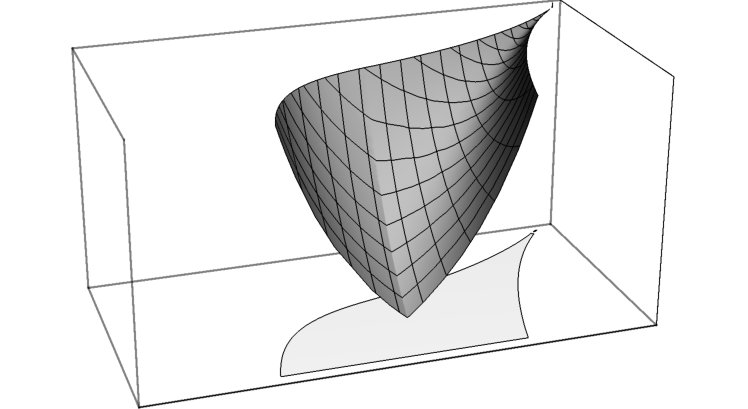 Figure 1
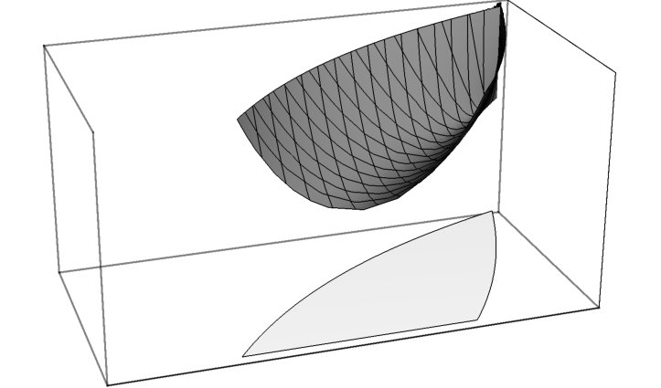 Figure 2
 Figure 3
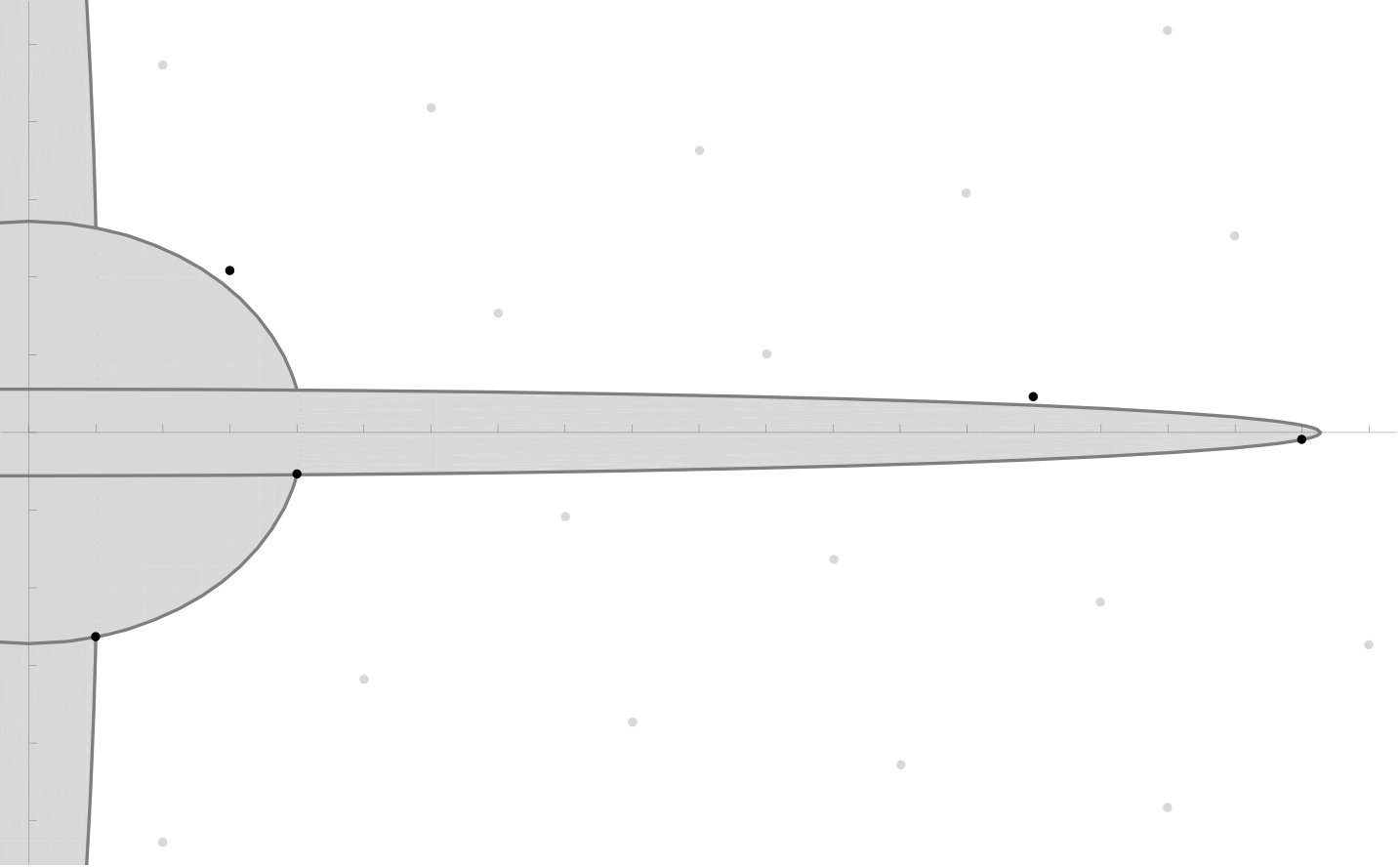 Figure 4
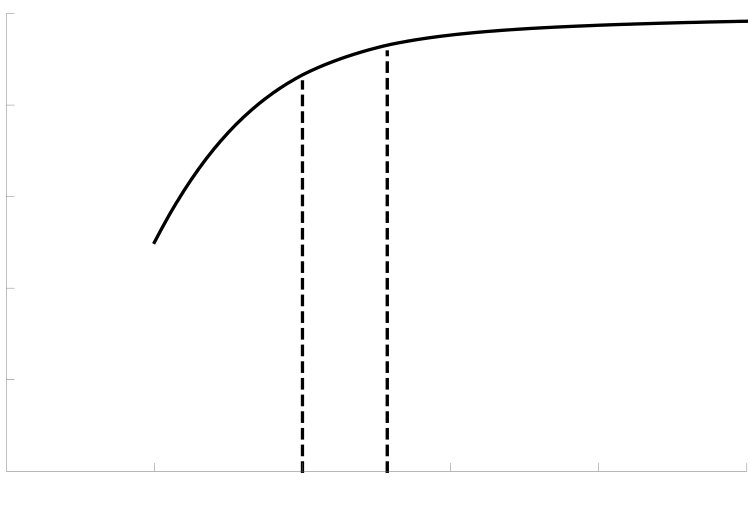 Figure 5
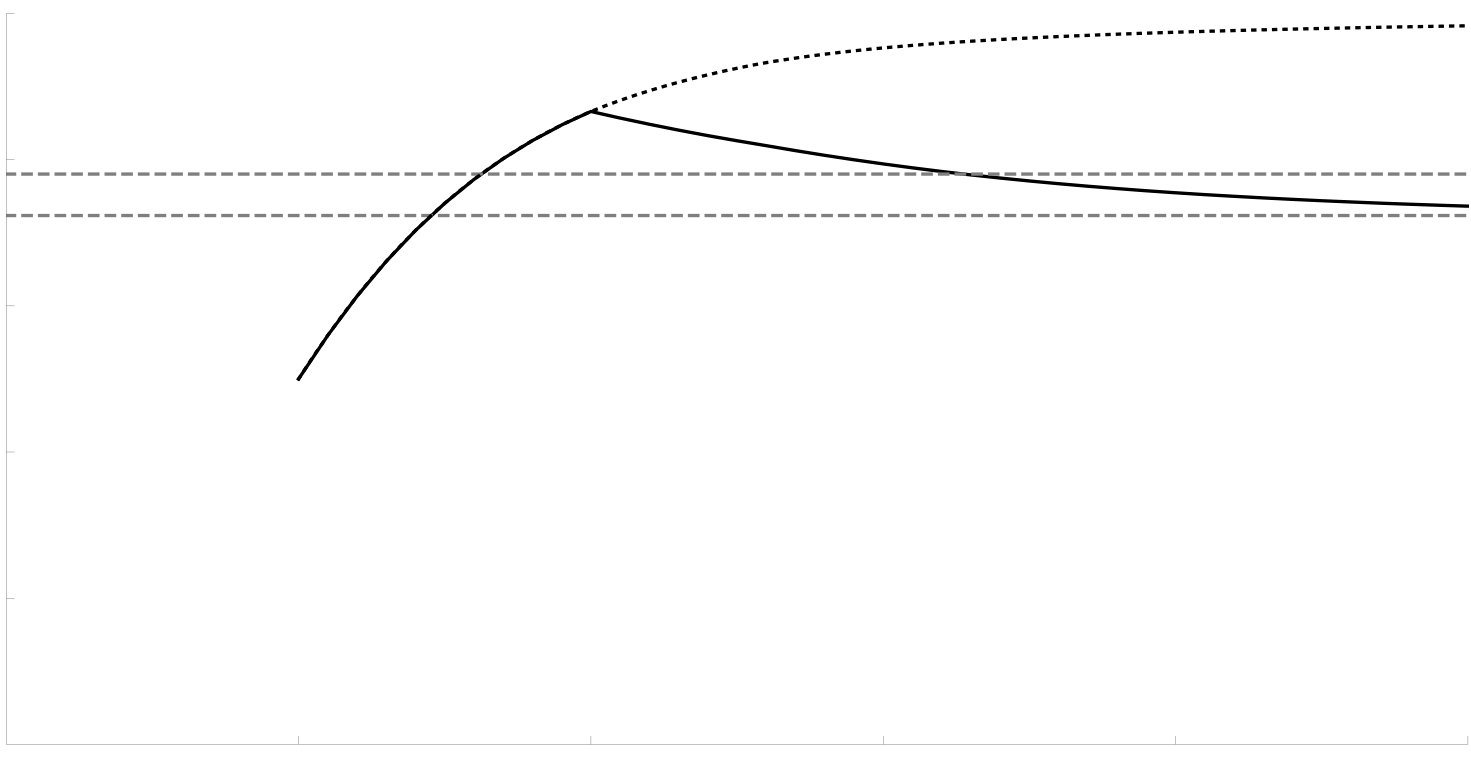 Figure 6
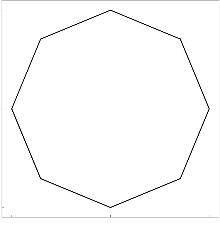 Figure 7
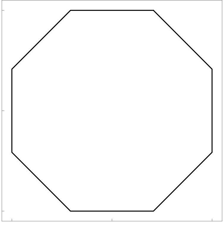 Figure 8
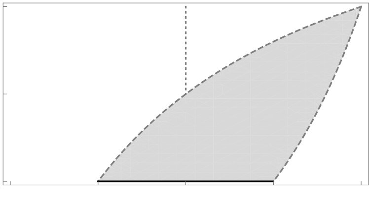 Figure 9
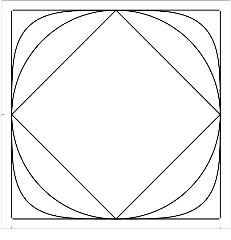 Figure 10
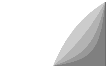 Figure 11
Peer Reviews
No public reviews on file for this paper yet. If you reviewed it on a platform where reviews are public (OpenReview, ICLR, NeurIPS, ICML), you can paste yours below so the community can read it here.
Videos
No videos yet. Explain this paper in a talk, walkthrough, or lecture? Add one.
On a theorem of Davenport and Schmidt
Nickolas Andersen
UCLA Mathematics Department, Box 951555, Los Angeles, CA 90095-1555
and
William Duke
UCLA Mathematics Department, Box 951555, Los Angeles, CA 90095-1555
Abstract.
This work is motivated by a paper of Davenport and Schmidt, which treats the question of when Dirichlet’s theorems on the rational approximation of one or of two irrationals can be improved and if so, by how much. We consider a generalization of this question in the simplest case of a single irrational but in the context of the geometry of numbers in , with the sup-norm replaced by a more general one. Results include sharp bounds for how much improvement is possible under various conditions. The proofs use semi-regular continued fractions that are characterized by a certain best approximation property determined by the norm.
Supported by NSF grant DMS 1701638.
1. Introduction
In 1842 Dirichlet [13] applied the pigeonhole principle to give good approximations of real numbers by rationals. One form of his theorem in one dimension is the following.
Dirichlet Approximation Theorem**.**
For and any there are such that and
Davenport and Schmidt [10] considered those for which an improvement of this result is possible, at least when we only require that be sufficiently large. More precisely, let be the largest number with the property that if then for every sufficiently large (depending only on ), there are integers with and while if there are arbitrarily large for which no such exist. If then we say that an improvement on Dirichlet’s theorem is possible for this . Clearly for rational so we only consider irrational .
An easy direct argument proves the fact, perhaps surprising at first, that any irrational for which must be badly approximable. For to be badly approximable means that for some we have for all relatively prime integers with . Davenport and Schmidt gave another proof of this that also shows that, conversely, an improvement on Dirichlet’s theorem is possible for every badly approximable number. They deduced this from a formula for given in terms of the regular continued fraction expansion of Recall that an irrational has a unique infinite regular continued fraction expansion
[TABLE]
where the partial quotients satisfy and for . Also define , while for let
[TABLE]
Theorem**.**
(Davenport-Schmidt [10]) For any irrational we have that
[TABLE]
An immediate consequence of (1.3) is that the irrational for which Dirichlet’s theorem can be improved are precisely those whose continued fraction have bounded partial quotients. This condition is well-known to be equivalent to being badly approximable [49, p. 22]. Real quadratic irrationalities are precisely those whose regular continued fraction expansions are eventually periodic, so they are badly approximable. On the other hand, they are the only known examples that are algebraic. A continued fraction discovered by Euler [15] provides an explicit example of an irrational (in fact transcendental) number that is not badly approximable, namely
[TABLE]
By a well-known result of Khintchine [24, Thm 29] badly approximable numbers, although uncountable, are rare in the sense of measure theory. Thus we have the following.
Corollary**.**
The set of real irrationals for which Dirichlet’s theorem can be improved is uncountable and has Lebesgue measure zero.
Another consequence of the formula (1.3) is a bound for how much the Dirichlet theorem can be improved when it can be improved at all.111 For further results about the set of values of see [22] and the references therein. See also our §12.
Corollary**.**
The smallest value of is given by
[TABLE]
when .
2. Improving the Minkowski approximation theorem
Davenport and Schmidt used their theorem as a starting point to obtain results that pertain to the Dirichlet theorems about approximating two numbers simultaneously and later more generally [11] (see also [48]). In this paper we will consider a different kind of generalization of Dirichlet’s results, one that was conceived of by Hermite and Minkowski.
Let be a fixed norm on and its unit ball. Define the stretched norm for by
[TABLE]
The following generalization of Dirichlet’s theorem follows from the work of Minkowski. Although it was not stated directly by him, for the purposes of this paper we will refer to it as the Minkowski approximation theorem (in two dimensions).
Minkowski Approximation Theorem**.**
For a fixed norm on let be the minimal area of a parallelogram with one vertex at the origin and the other three on the boundary of . Fix . Then for any real there exist integers with such that
[TABLE]
Note that for this result we are not restricting to be an integer. It is not hard to see that for the sup-norm the Minkowski approximation theorem implies Dirichlet’s theorem. In this case
The idea of generalizing Dirichlet’s theorem to other norms goes back at least to Hermite [19]. He applied (2.2) for the Euclidean norm, for which , together with the inequality between arithmetic and geometric means. The resulting inequality implies that for any irrational there are infinitely many integers with such that
[TABLE]
improving upon the corresponding upper bound given by Dirichlet’s theorem. Later Minkowski [33, 36] showed that (2.2) with the 1-norm given by and for which , implies (2.3) with replaced by .
Given these results of Hermite and Minkowski, it is natural to study the generalization for any norm of the quantity from the Davenport-Schmidt theorem. We want this generalization to measure to what extent the Minkowski approximation theorem (2.2) can be improved for a particular . Hence for a fixed norm , let be the largest number with the property that if then for every sufficiently large there are with such that
[TABLE]
while for there are arbitrarily large for which no such exist. For a given norm we say that the Minkowski approximation theorem can be improved for irrational if A straightforward argument shows that when is the sup-norm, for in the Davenport–Schmidt theorem.
We have only been able to obtain satisfactory results about if we make the assumption that for all the norm satisfies
[TABLE]
At least for the study of , we may assume without any further loss of generality that the norm also satisfies
[TABLE]
Definition 1**.**
Say that a norm is strongly symmetric if it satisfies (2.4) and (2.5).
The most important strongly symmetric norms are the -norms. For and a fixed the -norm is defined by
[TABLE]
while Denote the corresponding by , by and by Other interesting examples are the two unique strongly symmetric norms whose unit balls are regular octagons: and (see Figure 1).
Our first result generalizes the first corollary of the theorem of Davenport and Schmidt. It shows that for a strongly symmetric norm the set of irrationals for which the Minkowski approximation theorem can be improved, while uncountable, is small in the sense of measure theory.
Theorem 1**.**
Fix a strongly symmetric norm . Then the set of all real irrationals for which Minkowski’s approximation theorem can be improved is uncountable and has Lebesgue measure zero.
Next we have a uniform lower bound for for any strongly symmetric norm and any irrational .
Theorem 2**.**
For any strongly symmetric norm and any irrational we have that
[TABLE]
Equality in (2.6) can hold for the 1-norm. This follows from the next result since For simplicity say that an irrational is well approximable if it is not badly approximable.
Theorem 3**.**
For any strongly symmetric norm the smallest value of for a well approximable is
We will see in the proof of Theorem 3 that for any whose regular continued fraction has partial quotients that are eventually strictly increasing, for example from (1.4). For the -norm we can go further and identify the smallest value of for any irrational .
Theorem 4**.**
For the -norm the smallest value of for an irrational is when and is
[TABLE]
when The value in (2.7) is attained when
The value of is given below in (4.2). See Figure 2 for graphs of and the minimum value of It is not the case that the Minkowski approximation theorem can always be improved for each badly approximable irrational, not even each real quadratic irrational. For example, we show at the end of §8 that
[TABLE]
Finding the norm or norms with the largest minimum value of among all strongly symmetric norms seems an interesting problem. The 2-norm has the largest minimum value of among all -norms. It can be shown that the minimum value of for both of the octagonal norms is (see the end of §10). Among all of the examples we have considered, the 2-norm provides the largest minimum (see Figure 2).
Remarks:
Results like ours involving continuously varying norms belong to the “parametric geometry of numbers,” an area that has recently seen a revival of activity stimulated by Schmidt and Summerer [50, 51]. See also [47] and its references.
The sequence from (1.2) represents a trajectory of the dynamical system on determined by the extended continued fraction map given by and for by
[TABLE]
It has an invariant measure with density function
[TABLE]
The ergodicity of this system, which is the natural extension of the usual continued fraction dynamical system, can be used to give a different proof that Dirichlet’s theorem cannot be improved for almost all real irrationals. An argument of [23], given as Lemma 5.3.11 of [9], allows one to conclude an almost all result for the special trajectories (1.2). Our proof of Theorem 1 proceeds along similar lines except that the trajectories of our dynamical system are determined by certain semi-regular continued fractions, which admit as partial numerators. The continued fractions we need are examples of -expansions, which have a well developed metrical theory again based on the ergodic theorem. For some remarks on the connection between these dynamical systems and the geodesic flow on see §12.
The second corollary of the Theorem of Davenport and Schmidt and our generalization, Theorem 4, require for their proofs information about all, rather than almost all trajectories. Other aspects of the continued fractions we use are needed, including a best approximation property given in terms of the norm, in order to be able to analyze in detail each individual trajectory.
3. The continued fraction associated to a norm
We want to give a generalization of the formula (1.3) of Davenport and Schmidt and for that we require, as previously mentioned, certain infinite semi-regular continued fraction expansions. Such a continued fraction has the form
[TABLE]
where and for all and for infinitely many . For any the convergent of this continued fraction
[TABLE]
uniquely defines relatively prime integers with , where and Tietze ([55], see also [43, p. 135]) showed that there is an irrational to which such a continued fraction converges, meaning that
The continued fraction we need is characterized by a best approximation property stated in terms of the given strongly symmetric norm.
Definition 2**.**
Say that a rational number where is a best approximation to with respect to the norm if there is a depending only on such that
[TABLE]
for all rational .
In the case of the sup-norm Definition 2 is equivalent to the usual one that states that a rational number with is a best approximation to an irrational if for all rational numbers with we have
[TABLE]
(see Lemma 6.1 below).
Theorem 5**.**
Fix a strongly symmetric norm . Every irrational has a unique semi-regular continued fraction expansion whose convergents are precisely the best approximations to with respect to .
We will refer to this continued fraction as the -continued fraction of and, for the -norm, as the -continued fraction of For the sup-norm the -continued fraction is closely related to, but not always equal to, the regular continued fraction. Suppose that
[TABLE]
is the regular continued fraction of an irrational . Recall that Lagrange showed ([25], see also [43, §15]) that every best approximation in the usual sense is a convergent of the regular continued fraction of and that every convergent, except possibly , is a best approximation to . In view of Theorem 5, (3.2) coincides with the -continued fraction of if and only if . If the -continued fraction of is
[TABLE]
This is an example of a singularization, which has the effect of contracting the regular continued fraction by removing and the convergent , which is not a best approximation to in this case. This well-known exceptional case does not occur for the -continued fraction. With this one possible exception, however, the convergents of the -continued fraction and those of the regular continued fraction coincide.
For any , the inequality between arithmetic and geometric means immediately gives that a necessary condition for a regular convergent of an irrational to be a convergent of the -continued fraction is that
[TABLE]
For , when the right hand side is , Minkowski [34] showed that (3.4) is also sufficient.
Just as the formula (1.3) is given in terms of the sequence coming from the regular continued fraction, our generalization will be given in terms of a sequence determined by our continued fraction . Namely, for a fixed norm we define and , while for we let
[TABLE]
For a general strongly symmetric norm we will express in terms of these numbers in §7 below. For the -norm the formula is completely explicit and we give it here. For with let
[TABLE]
while when set
Theorem 6**.**
Fix For any irrational whose -continued fraction is (3.1) we have that
[TABLE]
where are given above in (3.5).
The -continued fraction of an irrational for any strongly symmetric norm is an example of an -expansion. Their theory has been developed by Kraaikamp [28] and others (see also [4], [9] and [26]). Recall the definition of and from (2.9) and (2.10). A Borel set is called a singularization area if and if
- (i)
and 2. (ii)
where
The -expansion of an irrational is obtained from the regular continued fraction (1.1) by changing
[TABLE]
for each such that . Note that implies that by (i). Also (ii) implies that this procedure is unambiguous. The result is a unique semi-regular continued fraction for whose convergents are precisely those regular convergents where is such that . For example, the -continued fraction discussed above is the expansion for . As usual, we denote by in the case of the -norm (see Figure 3).
Theorem 7**.**
Fix a strongly symmetric norm . There exists a singularization area so that the -continued fraction of any irrational is the -expansion of .
Remarks: At the beginning of the paper [33], Minkowski states without proof several of the main properties of the -continued fraction for any , including the best approximation property. Our proof of Theorem 5, which allows for to be any strongly symmetric norm, was strongly influenced by his ideas. As previously mentioned, Minkowski [34] also gave the remarkable result that for the 1-continued fraction the necessary condition (3.4) is also sufficient. Unsurprisingly, this also follows from our arguments. In addition, the 2-continued fraction has actually been studied since the time of Hermite [18], especially by Humbert [20, 21]. It is also closely connected to the improper modular billiards studied in [1]. It was shown in [27] that the 1-continued fraction (known as Minkowski’s diagonal continued fraction) is an -expansion. For related work on the 1-continued fraction see [40]. That the -continued fraction for is also an -expansion seems to be new.
In the next section we will review some basic facts from the geometry of numbers in the case we need, namely in two dimensions. Seven sections, each with the proof of one of our theorems, follow afterward. The theorems will be proven in the following order:
[TABLE]
Some concluding remarks are then given. Finally, an appendix contains a number of technical lemmas and their proofs that we will refer to as needed in the main body of the paper.
4. Geometry of numbers
As above let be a fixed norm on . This means that for we have
- (i)
and if and only if 2. (ii)
for 3. (iii)
.
The unit ball of the norm is
[TABLE]
This is open, bounded, convex and symmetric around 0 and every such body arises as the unit ball of some norm (see e.g. [52]). Denote by the Lebesgue measure of on . It is convenient to define the stretched ball for
[TABLE]
Let be a (full) lattice. By the determinant of , denoted , we mean for any whose rows give a -basis for . The lattice is admissible for if contains no other points of than . The following result is fundamental [36]:
Minkowski’s First Convex Body Theorem**.**
If is admissible for then
[TABLE]
The critical determinant of , denoted or simply , is the infimum of all determinants of lattices admissible for . Building on work of Minkowski [35, 37], Mahler [29] proved that lattices with determinant actually exist, and these are called critical lattices. Minkowski’s first convex body theorem implies that
[TABLE]
This is sharp for the 1-norm and the sup-norm.
Apparently, if we wish to evaluate exactly we must also know exactly. Finding the critical determinant of a given is the main problem of the geometry of numbers in Although the -dimensional version of this problem is apparently intractable in general, here it is approachable. For a given critical lattice for the boundary of must contain a -basis for as well as their sum . Furthermore, the lattice generated by any pair of points with on the boundary of is admissible for (see [7, Thm XI p. 160]). Therefore, as Minkowski already knew, computing amounts to solving the (generally quite difficult) calculus problem of minimizing the area of a parallelogram with one vertex at the origin and the three others on the boundary of . This justifies our definition of in the statement of the Minkowski approximation theorem.
Next we review what is known about the value of for all . Let
[TABLE]
where satisfies . A modification of a conjecture of Minkowski [37, p. 51–58] made by Davis [12] states that
[TABLE]
Furthermore, there is a unique value so that when , while otherwise . Many mathematicians obtained partial results, among them Mordell [39], Davis [12], Cohn [8], Watson [56, 57] and Malyshev [31]. Building on their work, the proof of the full conjecture was finally completed by Glazunov, Golovanov and Malyshev [16].
In the case of the -norm parallelograms that minimize the area may be given explicitly. For we may take the parallelogram with vertices at where
[TABLE]
For or we may take
[TABLE]
where again solves Except when or these parallelograms are unique up to obvious symmetries. When or there are infinitely many essentially different minimizing parallelograms. They are easily parameterized. For example, when all are obtained by rotating the standard hexagonal lattice coming from (4.3).
Minkowski’s method can be restated as saying that is the minimal area of an affinely regular symmetric hexagon inscribed in . A useful alternative due to Reinhardt [46] is that is the minimum area of a symmetric convex circumscribed hexagon (see also [7, p. 239] or [17, Thm 2 p. 243]). Using this fact, that he also found independently, Mahler [30] computed for the regular octagon from Figure 1. Thus we also have , obtained by scaling.
5. A Minkowski-type algorithm
In this section we will prove Theorem 2. First we give a needed definition. A minimal basis for a lattice with respect to a norm is a -basis for with the property that
[TABLE]
For let
[TABLE]
Obviously has determinant one.
To prove Theorems 2 and 5 we require an algorithm that constructs a sequence of points and positive numbers such that gives a minimal basis for with respect to We also want to have the smallest norm among non-zero points in for any . We will start with and . Roughly speaking, given , to find the new point and the associated , we simultaneously expand in the -direction while shrinking in the -direction in a such a way that remains on its boundary until we encounter . We then repeat this procedure starting with (see Figure 5). Our algorithm will produce pairs of lattice points in that are linearly independent over and on a ball for which is admissible. First we need to know that they give a basis for
Lemma 5.1**.**
Let be irrational and be a fixed strongly symmetric norm. Suppose that lie on the boundary of for some and are linearly independent over . If is admissible for then gives a -basis for .
Proof.
Consider the sublattice of generated by these lattice points. By Minkowski’s first convex body theorem its index in can only be 1 or 2. In the latter case suppose that and where , so If were even and odd we would have that is even and so would be a non-zero point in . A similar argument disallows being even and odd. Thus and are either both even or both odd. Similarly and are either both even or both odd. In any case
[TABLE]
are distinct points of . As is convex they must lie on the boundary of . It follows that must be a parallelogram and strong symmetry implies it is a stretched ball for either the 1-norm or the sup norm. As the corners and midpoints of the sides are lattice points we would have to have that contains points of the -axis, i.e. would be rational. ∎
In the next lemma we make the whole process precise. Clearly to represent any we may assume that
Lemma 5.2**.**
Fix a strongly symmetric norm and an irrational . There is a sequence tending to and for each there is a with the following properties. For each
- (i)
* and ,* 2. (ii)
* gives a minimal basis for with respect to ,* 3. (iii)
for any there is no different from with and
[TABLE]
Proof.
Consider for the ball
[TABLE]
for which Suppose that is admissible for . Now by Lemma A.1
[TABLE]
Thus, as long as , by Minkowski’s first convex body theorem there will be a maximal for which is admissible for . For any of the resulting with , we have by Lemma 5.1 that gives a minimal basis for with respect to
Let . Then is admissible for . Let be maximal for which is admissible for . Our assumption that implies that we can take as a solution to .
Now is admissible for and so we find maximal so that is admissible for . That with strict inequality is assured by our choice of . Among the finitely many with there will be unique one with maximal since is irrational. We let be this point. Clearly and .
We continue this process to construct and . That we have is guaranteed by choosing among the new points on the boundary the one with maximal -coordinate. From the form of , where is irrational, it follows that and for each and that this process never terminates.
We will have all the stated properties of and once we show that . We have by Lemma A.1 and Minkowski’s first convex body theorem again that for each
[TABLE]
Thus as are integers. ∎
Proof of Theorem 2
Observe that as defined by (5.2), with and from Lemma 5.2, contains a parallelogram of area 2 since is a minimal basis for with respect to Therefore
[TABLE]
where to get the second inequality we have applied Minkowski’s bound (4.1). Since as we have that
[TABLE]
thus proving Theorem 2. ∎
6. The continued fraction
Next we relate to each other the two definitions of best approximation given in and below Definition 2.
Lemma 6.1**.**
If the fraction with is a best approximation of an irrational with respect to a strongly symmetric norm then it is a best approximation in the usual sense. Conversely, if with is a best approximation of an irrational in the usual sense it is a best approximation with respect to the sup-norm.
Proof.
Suppose that there is a such that with implies
[TABLE]
If then by Lemma A.1.
Conversely, suppose that and implies that . Choose such that and note that such a
If and then
[TABLE]
If then
[TABLE]
This finishes the proof. ∎
Proof of Theorem 5
For any write , where and Suppose that is irrational. In the notation of Lemma 5.2 (taking there ) for write . For define
[TABLE]
and set . We know by Lemma 5.2 that for each there is a positive integer and so that
[TABLE]
This also holds for if we set Clearly for
[TABLE]
The numerator and denominator of the convergents
[TABLE]
of our continued fraction are determined recursively for through
[TABLE]
It is easy to see that for
[TABLE]
By (6.1) and (6.5) for each we get that
[TABLE]
By Lemma 5.2 the basis of rows of is minimal for the norm . Choose any . By (iii) of Lemma 5.2 for any we have
[TABLE]
Conversely, suppose that is a best approximation to with respect to , and write . Then for some , we have for all . By Lemma 5.2 it cannot happen that since in that case we would have to have and so . Also we cannot have that for any On the other hand, if is such that , then by Lemma 5.2 we have . It follows that the convergents are precisely the best approximations to with respect to .
That the continued fraction converges to now follows from the first statement of Lemma 6.1 and Lagrange’s theorem mentioned below Theorem 5, since they imply that each convergent of our continued fraction is a convergent of the regular continued fraction. It remains to show that it is semi-regular. Since is irrational we need only show that for all . This will follow once we relate the from (3.5) to the points , which is also needed to prove our generalization of (1.3).
Lemma 6.2**.**
For from (6.6) and from (3.5) we have for that
[TABLE]
Proof.
The proof is an adaptation to more general continued fractions of standard arguments used for regular continued fractions (see [49]).
To start with, by (6.6)
[TABLE]
[TABLE]
Together with (6.3) and (6.4), this yields the following formal identity between rational functions with variables :
[TABLE]
The complete quotient of the expansion is defined recursively by and for through
[TABLE]
It follows that for we have
[TABLE]
By (6.11) upon setting the variable and using (6.12) we derive that
[TABLE]
Next solve this equation for and use (6.10) with in place of to get
[TABLE]
From (6.12) we have
[TABLE]
so by (3.5)
[TABLE]
The first formula of (6.8) now follows from (6.9) and (6.13).
To prove the second formula of (6.8) start with from (6.6). By (3.5) we have that while for
[TABLE]
Using (6.4) we see that satisfies the same recurrence. ∎
We now finish the proof of Theorem 5 by showing that our expansion is semi-regular. Suppose that we had and for some We would then have from (6.14) that and so from (6.15) that
[TABLE]
which is impossible. This completes the proof of Theorem 5.∎
7. A formula for
We will deduce Theorem 6 from a formula for for any strongly symmetric norm given in terms of the quantities . As usual, we may identify the space of all lattices of determinant one with where and by means of
[TABLE]
Let be the set of such that
[TABLE]
For let
Lemma 7.1**.**
The map given by
[TABLE]
is a continuous bijection.
Proof.
The inverse of is given by
[TABLE]
By Lemma A.3 we see that exists and is uniquely determined by the condition ∎
The function
[TABLE]
is easily seen to be continuous on .
The following is our generalization of the formula (1.3).
Lemma 7.2**.**
Fix a strongly symmetric norm. For any irrational whose continued fraction associated to the norm is (3.1) we have that
[TABLE]
where are given above in (3.5).
Proof.
Fix an and write as before . Let
[TABLE]
where and . Recall that by (i) of Lemma 5.2 we know that
[TABLE]
Lemmas 7.1 and 6.2 now imply that
[TABLE]
where was defined in (6.2). Note that in this case By strong symmetry of the norm we have . Hence
[TABLE]
Now we need to show that
[TABLE]
For let be such that . By Lemma 5.2 we have that
[TABLE]
and by Lemma A.5 we have that
[TABLE]
Now apply the first inequality in (5.3) to establish (7.6) and therefore finish the proof of Lemma 7.2. ∎
Proof of Theorem 6
To conclude formula (3.6) from Lemma 7.2, first observe that for the -norm with we have from (7.4) that for the value of that makes the rows of have the same norm is given by
[TABLE]
The corresponding value of from (7.5) is
[TABLE]
giving (3.6). The case is immediate. This completes the proof of Theorem 6.∎
8. -expansions
To prove Theorem 7 we want to characterize in terms of the norm those convergents of the regular continued fraction of an irrational that are also convergents of the continued fraction of associated to a strongly symmetric norm . We will use the notation and results of Lemma 5.2. Write for points coming from this norm with corresponding and let be the points coming from the convergents of the regular continued fraction of . Furthermore, the partial quotient is associated to while is associated to .
Lemma 8.1**.**
For a fixed there are integers and with and so that for each
[TABLE]
where for all , while for we have
[TABLE]
Proof.
The integers are determined recursively for by
[TABLE]
It is easy to check using (8.1) and (8.2) that and satisfy for fixed and the recurrence relations
[TABLE]
The claim of the lemma follows from a straightforward inductive argument. ∎
The following result will be used to characterize those convergents of the regular continued fraction that occur as convergents in the continued fraction associated to the norm.
Lemma 8.2**.**
For let and be such that and . Then
- (i)
. 2. (ii)
There is a unique such that , and if and only if
[TABLE]
If this holds we have that 3. (iii)
* if and only if *
Proof.
We know that and that for each we have for some and for some We can check directly that if and only if
By Lemma 8.1 for we have
[TABLE]
By Lemma 5.2 we have and hence
[TABLE]
by Lemma A.4. Thus we have
[TABLE]
so by Lemma 8.1 we have that either or
Now by Lemma A.3 applied to the norm and using that
[TABLE]
there is a (indeed ) so that
[TABLE]
In case we have by (8.7) and (8.3)–(8.4). By (8.5) we have that
[TABLE]
so by Lemma 5.2 we must have
[TABLE]
If we have and so that and
[TABLE]
at least when , since then the -coordinate of is strictly larger than that of and so by Lemma 5.2 strict inequality must hold. ∎
Proof of Theorem 7
Lemma 8.2 gives instructions for obtaining the sequence of convergents of associated to the norm from the sequence of regular convergents of , namely
[TABLE]
where is such that , and
[TABLE]
We must define a singularization area that encodes both of these instructions. Let and be as in Section 7. For each we write
[TABLE]
and we define
[TABLE]
The portion of that lies on the -axis encodes the rule (8.9). Suppose that and let . Then Lemmas 7.1 and 6.2 imply that and , with defined by . So the condition on the right-hand side of (8.8) is equivalent to . It follows that (8.8)–(8.9) are encoded by the rule
[TABLE]
It is helpful to have some more concrete information about the set . For a generic norm it is difficult to describe explicitly, so we will relate to the set , which is easy to describe. As usual, we denote by when is the -norm. We have
[TABLE]
as one can see by reducing the system of equations and inequalities
[TABLE]
defining . The interior of the set (8.12) agrees with the -region given in [28] for Minkowski’s diagonal continued fraction.
Lemma 8.3**.**
For any strongly symmetric norm we have .
Proof.
Since and are closed sets in the induced topology on , it suffices to show that a dense subset of is contained in . Suppose that with and , and write
[TABLE]
for the regular continued fractions of and . If we define
[TABLE]
then for . Since we have in the notation of Section 8, and for some we have and . Thus
[TABLE]
Let be such that , where denotes the -norm. By convexity of , the closed stretched ball contains the line segment connecting the points and . This line segment comprises all of the points in the same quadrant as with -coordinate between and , and with . Since the -coordinate of is between and and is outside the ball , we have
[TABLE]
By (8.8) and (8.11) it follows that . ∎
Lemma 8.3, together with the explicit description (8.12), shows that the set is a singularization area as defined above Theorem 7. This fact and (8.11) together prove Theorem 7.∎
We also immediately obtain the following lemma, which we will use several times in the coming sections.
Lemma 8.4**.**
For every strongly symmetric norm , there is a neighborhood of the line segment with that does not intersect .
We finish this section with a quick proof of our claim (2.8) that
[TABLE]
The regular continued fraction expansion of is
[TABLE]
from which it follows that
[TABLE]
while from below and from above. The region comprises those points for which . The points are all outside , so the -continued fraction expansion of is the same as the regular continued fraction and thus . Since , we have
[TABLE]
9. Values of for well approximable numbers
We now prove Theorem 3, which gives the smallest value of for any strongly symmetric norm and well approximable.
Lemma 9.1**.**
Suppose that is well approximable. Then
Proof.
By definition, for any there are arbitrarily large so that for some
[TABLE]
For such a let and note that for any with
[TABLE]
for some with By Lemma A.1 if we have
[TABLE]
while for we have since . By the continuity of , for any there is an so that . It follows that and hence that ∎
To finish the proof of Theorem 3, we need to find well approximable for which
Lemma 9.2**.**
Suppose that the partial quotients of the regular continued fraction expansion of are eventually strictly increasing with . Then
[TABLE]
Proof.
If the regular partial quotients of are eventually strictly increasing, then for any the points all eventually lie within of the point . So by Lemma 8.4, the points are outside for sufficiently large . Thus
[TABLE]
Finally, , therefore . ∎
10. Values of for any irrational
Proof of Theorem 4
Fix . Throughout the proof let
[TABLE]
denote the -continued fraction expansion of and define and as in (3.5). By Theorem 6 it suffices to show that for every we have
[TABLE]
and that there is at least one for which equality holds. In both cases the number on the right-hand side of (10.2) is . Since , we have
[TABLE]
It follows that for nonpositive , so if for infinitely many , the inequality (10.2) holds trivially. Thus we may assume that the -continued fraction expansion of has for all sufficiently large .
Lemma 10.1**.**
If then
[TABLE]
with equality only when .
Proof.
The inequalities
[TABLE]
both reduce to . It remains to show that
[TABLE]
This inequality is implied by the first inequality of (10.4) and
[TABLE]
which follows immediately from Hölder’s inequality. ∎
It is convenient to define
[TABLE]
Then
[TABLE]
If then is strictly increasing, so by Lemma 10.1 we have
[TABLE]
If then for all . In either case, we can use Lemma 9.2 to find examples of for which .
Suppose that , and let . The sequence associated to the regular continued fraction
[TABLE]
approaches as . By Lemma 8.4 it follows that the sequence associated to the -continued fraction of also converges to . Thus, for we have , which is the number in (2.7).
It remains to show that for every with for sufficiently large , we have for infinitely many . Since , the function is strictly decreasing, so by Lemma 10.1 it suffices to show that
[TABLE]
for infinitely many .
If there are infinitely many such that then for such we have and therefore . So we may suppose that for all sufficiently large . The following lemma covers the remaining cases.
Lemma 10.2**.**
Let and suppose that and for sufficiently large . If for infinitely many , then
[TABLE]
for infinitely many .
Proof.
Suppose that and for . Then for any with we have
[TABLE]
The lemma now follows from an easy computation. ∎
This completes the proof of Theorem 4.∎
We remark that it is sometimes possible to compute the minimum value of for other norms as well. The composition of strongly symmetric norms is, up to scaling, also strongly symmetric (see Lemma A.2). For instance, the norms and with regular octagonal unit balls mentioned in §1 can be given in terms of compositions of the 1-norm and the sup-norm. Explicitly,
[TABLE]
where These formulas, together with Mahler’s computation of the critical determinant of the regular octagon recalled at the end of §4 and Lemma 8.4, lead to the result referred to at the end of §1. The minimum of for is which is attained when
[TABLE]
For the minimal value is also , but now this is the value of and is attained when , for instance.
11. The dynamical system
The goal of this section is to prove Theorem 1. We employ the notation of Section 8. Say that is reduced with respect to the norm if and
[TABLE]
where the overline denotes the closure and was defined in (7.1). Let be the set of all that are reduced with respect to and define as
[TABLE]
where
[TABLE]
We will show that for all .
We want to apply the ergodic theory of -expansions as developed in [27]. For that we need to show that defined by (11.2) coincides with the set
[TABLE]
defined in Section 5 of [27], where
[TABLE]
The following equivalent description of reduced matrices is helpful.
Lemma 11.1**.**
A matrix is reduced if and only if
[TABLE]
Proof.
Clearly a matrix satisfying (11.1) also satisfies (11.3). Suppose satisfies (11.3). We will show that for all . If then
[TABLE]
Otherwise, if , say, then by the reverse triangle inequality
[TABLE]
This is strictly greater than if . If then
[TABLE]
This completes the proof since so . ∎
It follows that the set decomposes as , where
[TABLE]
See Figure 6 for the case .
Since the critical lattices for are among those for which two basis vectors and their sum all have equal norm, we will refer to the set
[TABLE]
as the potentially critical matrices. The next lemma describes the boundary of in terms of the distinguished subset
[TABLE]
of the potentially critical matrices.
Lemma 11.2**.**
The part of the boundary of that lies in is , where
[TABLE]
Proof.
The boundary of is , where
[TABLE]
Clearly is the part of adjacent to . The remaining set, , is the image of the set of satisfying
[TABLE]
If the -coordinate of is negative, then gives an element of , and
[TABLE]
Otherwise yields an element of ; in this case
[TABLE]
This completes the proof. ∎
Lemma 11.3**.**
The function is continuous on and assumes its maximum value on that set.
Proof.
The continuity statement is clear from the definition of . Say that a point in is a critical point if . For , let the points and be such that . Then
[TABLE]
where is the lattice generated by the unit vectors and . Thus is a critical point if and only if is a critical lattice, so by Lemma 11.2 all critical points lie on the boundary of . If critical points in exist, then we are done.
Suppose that a critical lattice corresponds to the point in the -plane. Then there exists a such that
[TABLE]
Then the matrix is in and satisfies . So if corresponds to a critical lattice , then the point is a critical point. ∎
That follows from the next lemma.
Lemma 11.4**.**
We have
[TABLE]
Proof.
We begin by showing that . For we have , so (2.9) simplifies to . We show that the boundary of maps to the boundary of under ; the lemma then follows by the continuity of on . Since and , it suffices to show that . Suppose that and that . Then
[TABLE]
Since this is clearly invertible, we conclude that .
We prove similarly. We have and for the straight line segments, so it suffices to show that . We will show that , using that
[TABLE]
Suppose that and that . Then
[TABLE]
which completes the proof. ∎
Let where was defined in (2.10).
Lemma 11.5**.**
Define and by (8.10) and (11.2). Then for almost all irrational the sequence is uniformly distributed over with respect to the measure .
Proof.
Since , Lemma 11.5 follows from Theorem 5.4.23 of [9] (see also [27]) and Theorem 7. ∎
Proof of Theorem 1
By Lemma 11.3, the function assumes the value at some point in . By Lemma 7.2 it follows that if and only if the sequence is infinitely often arbitrarily close to such a critical point. It follows from Lemma 11.5 that for almost all .
To finish the proof it suffices to show that there are uncountably many such . Since we already know Theorem 1 is true in the case of the sup-norm, suppose that is not the sup-norm. Then the lattice generated by and is not potentially critical, so we have . Thus any for which converges to has , and there are uncountably many such (for example, the set of with strictly increasing partial quotients).∎
12. Concluding remarks
In addition to the proof of Theorem 1, there are other applications of the metric theory of -expansions and ergodic theory to quantities related to For instance we may treat the distribution of the values of
[TABLE]
from Theorem 6. For almost all the distribution function
[TABLE]
exists for all For it can be evaluated explicitly, as was done for in Theorem 4 of [5]. In particular, for almost all
[TABLE]
exists where
[TABLE]
It is well known that a close connection exists between dynamical systems associated to various kinds of continued fractions and the geodesic flow on . See [14] and a discussion in [2] for more on this connection and for references to the literature. Roughly speaking, the natural extension of a continued fraction transformation can be identified with a cross section for the geodesic flow. For example, the transformation from (2.9) of the regular continued fraction’s natural extension gives a planar representation of the first return map and corresponds to the Liouville measure. Geodesics can be identified with (proper classes of) indefinite binary quadratic forms and a cross section with a reduction domain. The trajectories we study in this paper correspond to cuspidal geodesics or, equivalently, forms with one rational root.
Of course there is great interest in similar Diophantine problems about general indefinite forms and hence general geodesic trajectories. A prime example is the Markov problem [32] about the minima of such forms and their possible values; these values determine the Markov spectrum (see [3] and its references). The Lagrange spectrum is similarly defined using cuspidal trajectories; it is determined by the values of
[TABLE]
The Dirichlet spectrum is determined by the values of in [22] it is defined to be the set of values of There is a spectrum that is related to the Dirichlet spectrum in the same way that the Markov spectrum is related to the Lagrange spectrum. Like the Markov problem, its study involves general geodesic trajectories and their associated continued fractions. Again speaking roughly, we replace over cuspidal geodesics in the definition of by the supremum over all geodesics. Mordell [38] introduced this problem (actually an -dimensional version), which he posed as a kind of converse to Minkowski’s linear forms theorem. The case of two dimensions was treated in more detail by Szekeres [54], Oppenheim [41] and Burger [6]. This problem in higher dimensions has also attracted a lot of attention (see e.g. [44, 45, 53]).
It should be apparent that a general spectrum of this type can be defined for any strongly symmetric norm , not just the sup-norm, and that an associated reduction theory for indefinite binary quadratic forms can be developed that uses -continued fractions. For the 2-norm the problem was introduced by Oppenheim [42] and the relevant reduction theory was already found by Hermite. Minkowski developed the reduction theory for the 1-norm with Hermite’s theory in mind and certainly knew that a version could be based on the -norm for a general [36, footnote on p. 166]. However, outside of the sup-norm, only isolated aspects of the spectrum and reduction theory have been considered and only for the -norm for
Appendix A Lemmas about norms
Here we state and prove a number of simple technical lemmas that are referred to in the body of the paper. Here is a norm on with unit ball and For we define as above The lemmas give various properties of norms that satisfy the first condition (2.4) of strong symmetry. Note that if satisfies (2.4) then so does for any The first result is crucial and is used repeatedly in this paper.
Lemma A.1**.**
Suppose that satisfies (2.4). If and then we have that
[TABLE]
Proof.
To see this observe that if then hence by convexity. ∎
Lemma A.2**.**
If satisfy (2.4) then so does defined by
[TABLE]
Proof.
This follows easily using Lemma A.1. ∎
Lemma A.3**.**
Suppose that satisfies (2.4). The following properties hold.
- (i)
If and then for some unique we have
[TABLE] 2. (ii)
If and then for some unique we have
[TABLE]
Proof.
We only prove (i) as (ii) is a consequence of (i) applied to the norm
Existence: If take Otherwise for any define the continuous function by Now by Lemma A.1
[TABLE]
On the other hand, as . Because the existence of desired follows by the intermediate value theorem.
Uniqueness: Suppose that for with we have
[TABLE]
This implies that and that , which is not true. ∎
The following result is trivial in case the norm is strictly convex.
Lemma A.4**.**
Suppose that that satisfies (2.4), that we have and that and . Then for any
[TABLE]
Proof.
To see this note first that in order for equality to hold in (A.1) we must have that
[TABLE]
which implies that
[TABLE]
hence
[TABLE]
That this is impossible follows by a simple convexity argument using the locations of
[TABLE]
together with (2.4). ∎
Lemma A.5**.**
Suppose that that satisfies (2.4). For with and we have
[TABLE]
Proof.
Using the fact that the function is concave up and applying Lemma A.1 we get that
[TABLE]
By the defining properties of a norm we finish the proof. ∎
The reference list from the paper itself. Each links out to its DOI / PubMed record.
- 1[1] Andersen, N. & Duke, W., Markov spectra for modular billiards, to appear in Math. Annalen (2019).
- 2[2] Arnoux, P. & Schmidt, T.A., Cross sections for geodesic flows and α 𝛼 \alpha -continued fractions. Nonlinearity 26 (2013), no. 3, 711–726.
- 3[3] Bombieri, E., Continued fractions and the Markoff tree. Expo. Math. 25 (2007), no. 3, 187–213.
- 4[4] Bosma, W., Optimal continued fractions. Nederl. Akad. Wetensch. Indag. Math. 49 (1987), no. 4, 353–379.
- 5[5] Bosma, W. & Jager, H. & Wiedijk, F., Some metrical observations on the approximation by continued fractions. Nederl. Akad. Wetensch. Indag. Math. 45 (1983), no. 3, 281–299.
- 6[6] Burger, E. B., On a question of Mordell and a spectrum of linear forms. J. London Math. Soc. (2) 62 (2000), no. 3, 701–715.
- 7[7] Cassels, J. W. S., An introduction to the geometry of numbers. Die Grundlehren der mathematischen Wissenschaften in Einzeldarstellungen mit besonderer Berücksichtigung der Anwendungsgebiete, Bd. 99 Springer-Verlag, Berlin-Göttingen-Heidelberg 1959 viii+344 pp.
- 8[8] Cohn, H. Minkowski’s conjecture on critical lattices in the metric ( | ξ | p + | η | p ) 1 p superscript superscript 𝜉 𝑝 superscript 𝜂 𝑝 1 𝑝 (|\xi|^{p}+|\eta|^{p})^{\frac{1}{p}} , Ann. of Math. 51 (1950) 734–738.