A Coupled Oscillator Model for the Origin of Bimodality and Multimodality
Joseph D. Johnson, Daniel M. Abrams

TL;DR
This paper demonstrates that bimodal and multimodal distributions can naturally arise from repulsive coupling in oscillator models, challenging the assumption that natural distributions are typically unimodal.
Contribution
It introduces a rigorous analysis of how multimodality emerges from inhibitory coupling in variants of the Kuramoto model, expanding understanding of distribution shapes in coupled systems.
Findings
Multimodality can result from repulsive coupling dynamics.
The analysis applies broadly to various coupling functions.
Multimodal distributions emerge naturally in oscillator systems.
Abstract
Perhaps because of the elegance of the central limit theorem, it is often assumed that distributions in nature will approach singly-peaked, unimodal shapes reminiscent of the Gaussian normal distribution. However, many systems behave differently, with variables following apparently bimodal or multimodal distributions. Here we argue that multimodality may emerge naturally as a result of repulsive or inhibitory coupling dynamics, and we show rigorously how it emerges for a broad class of coupling functions in variants of the paradigmatic Kuramoto model.
Click any figure to enlarge with its caption.
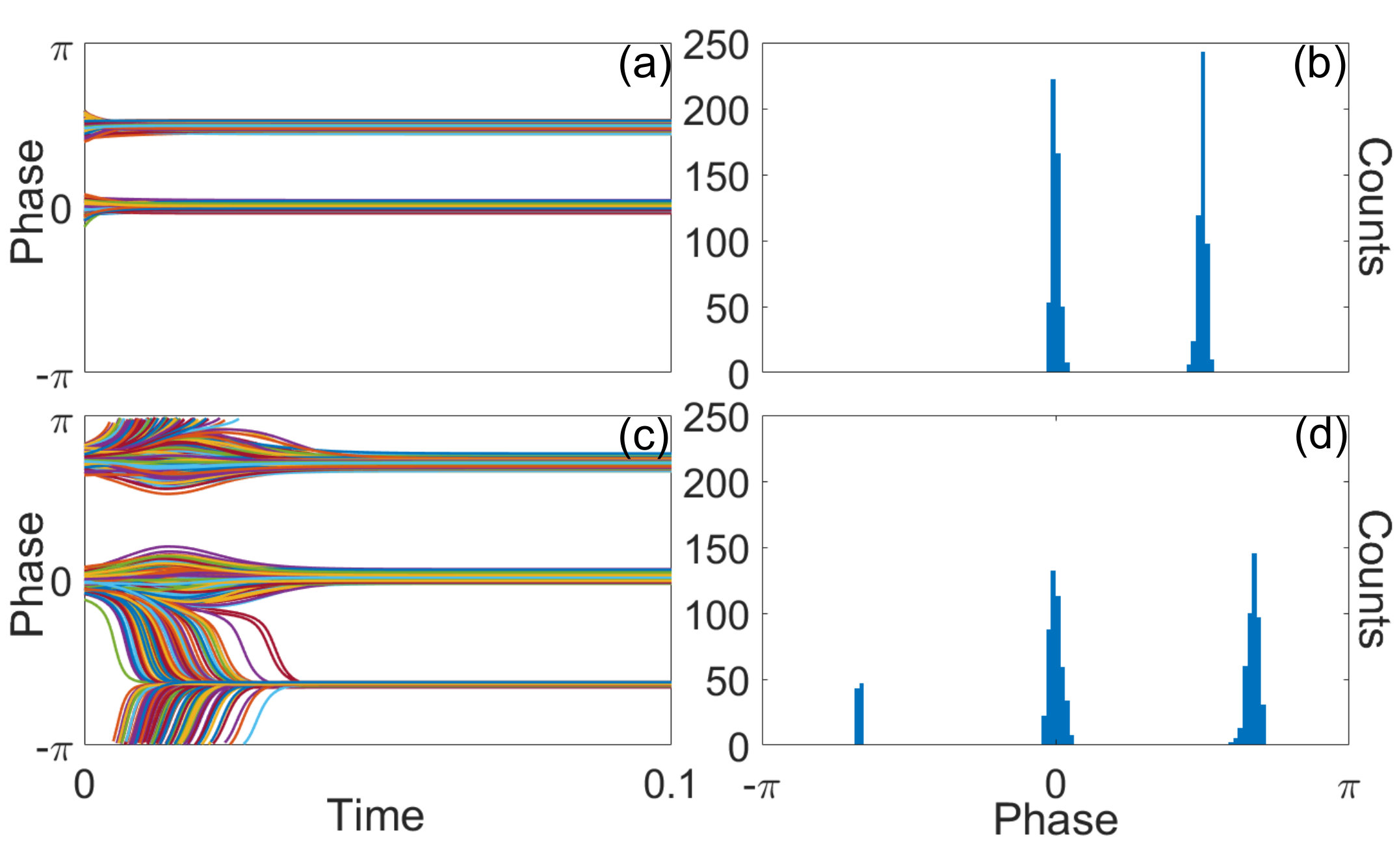 Figure 1
 Figure 2
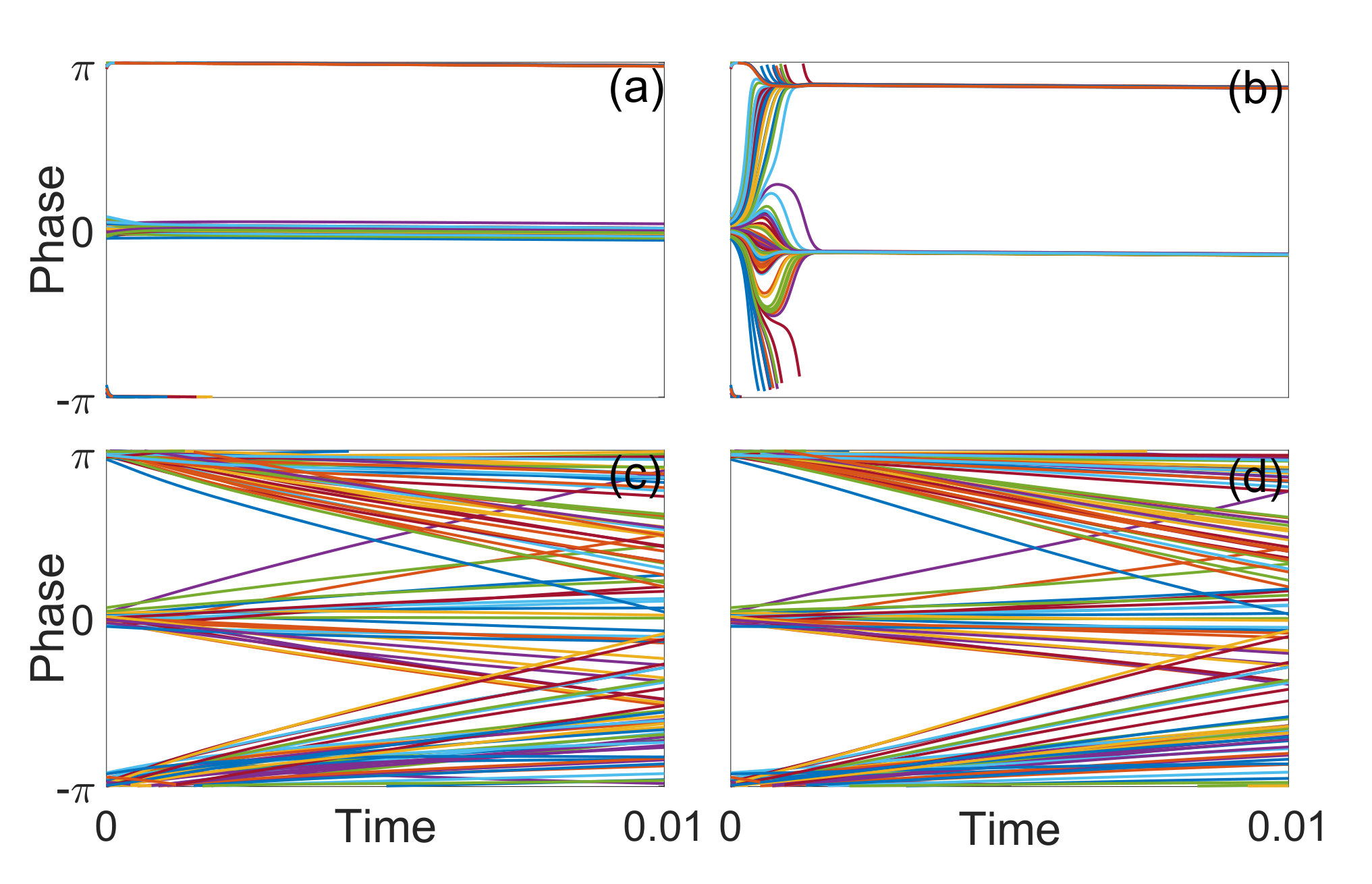 Figure 3
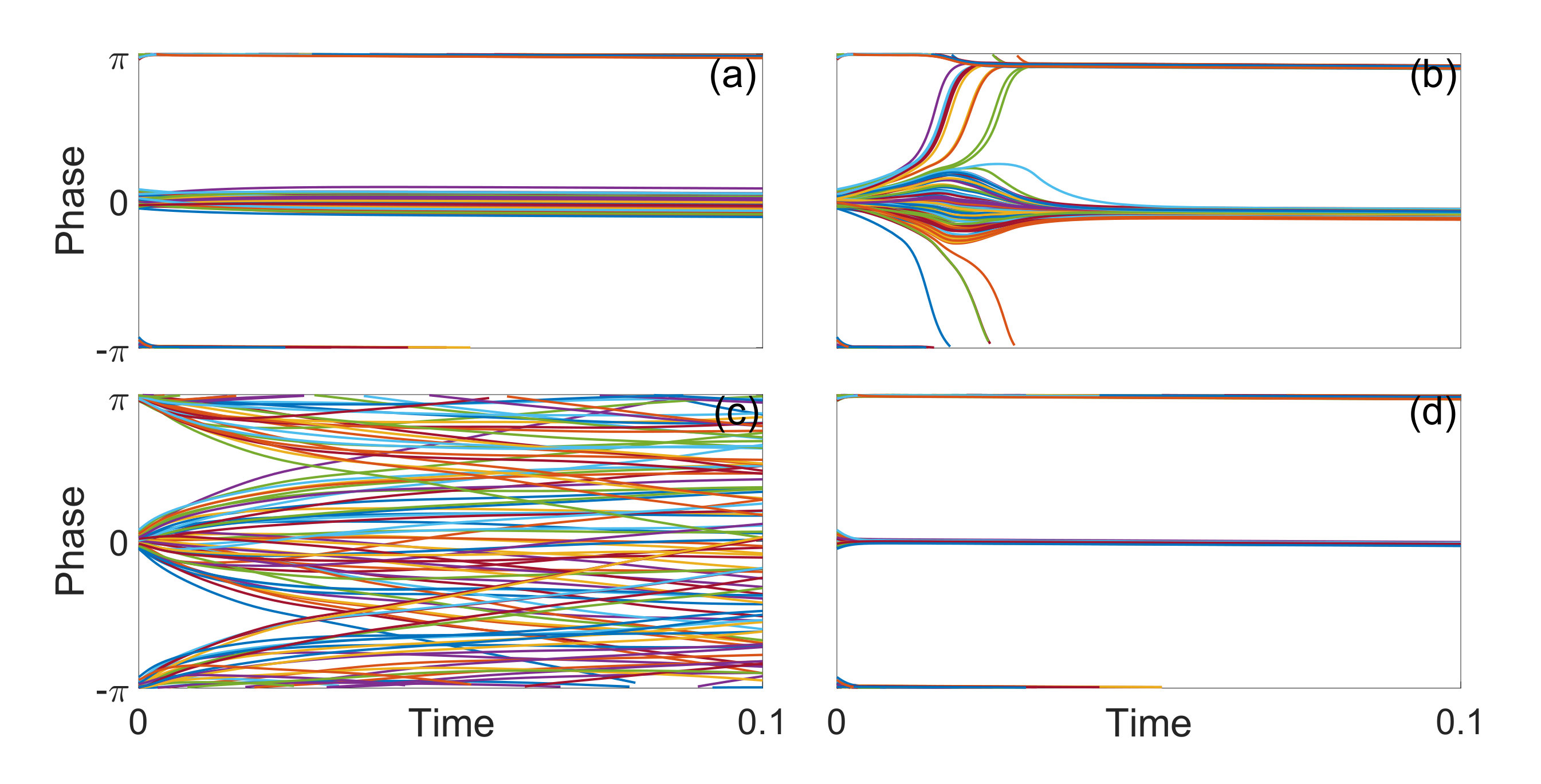 Figure 4
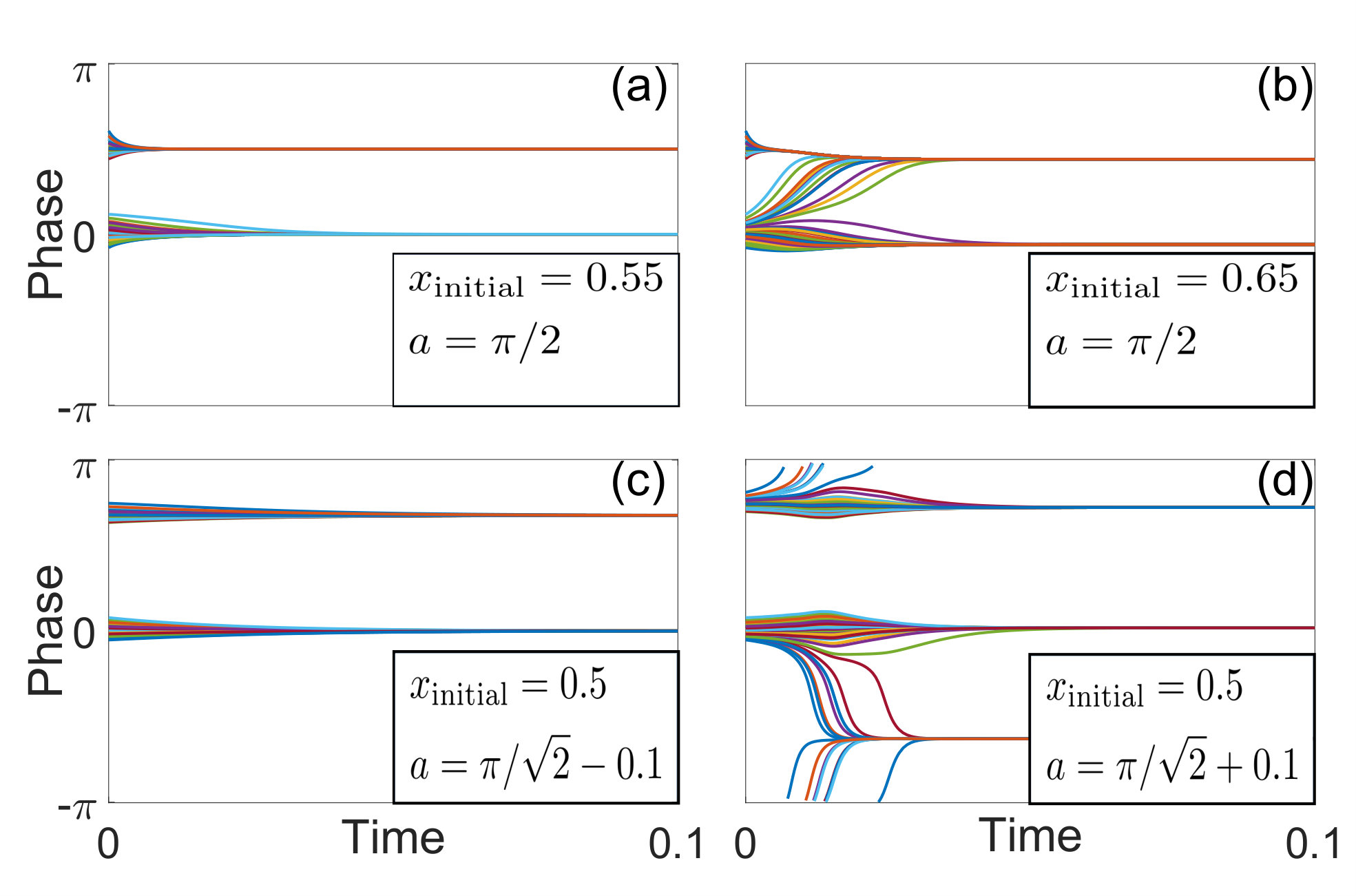 Figure 5
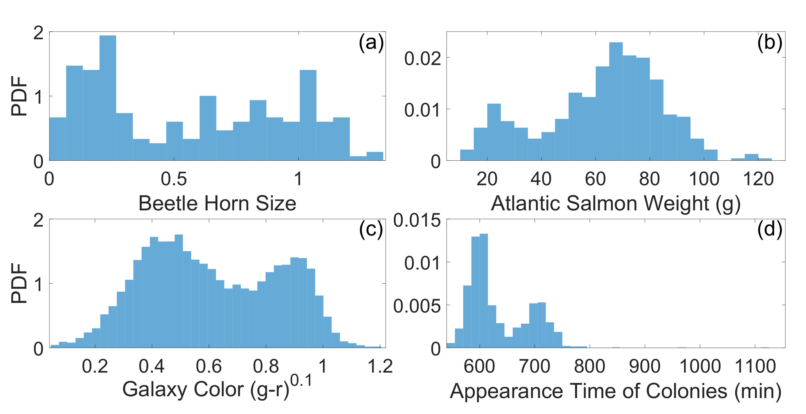 Figure 6
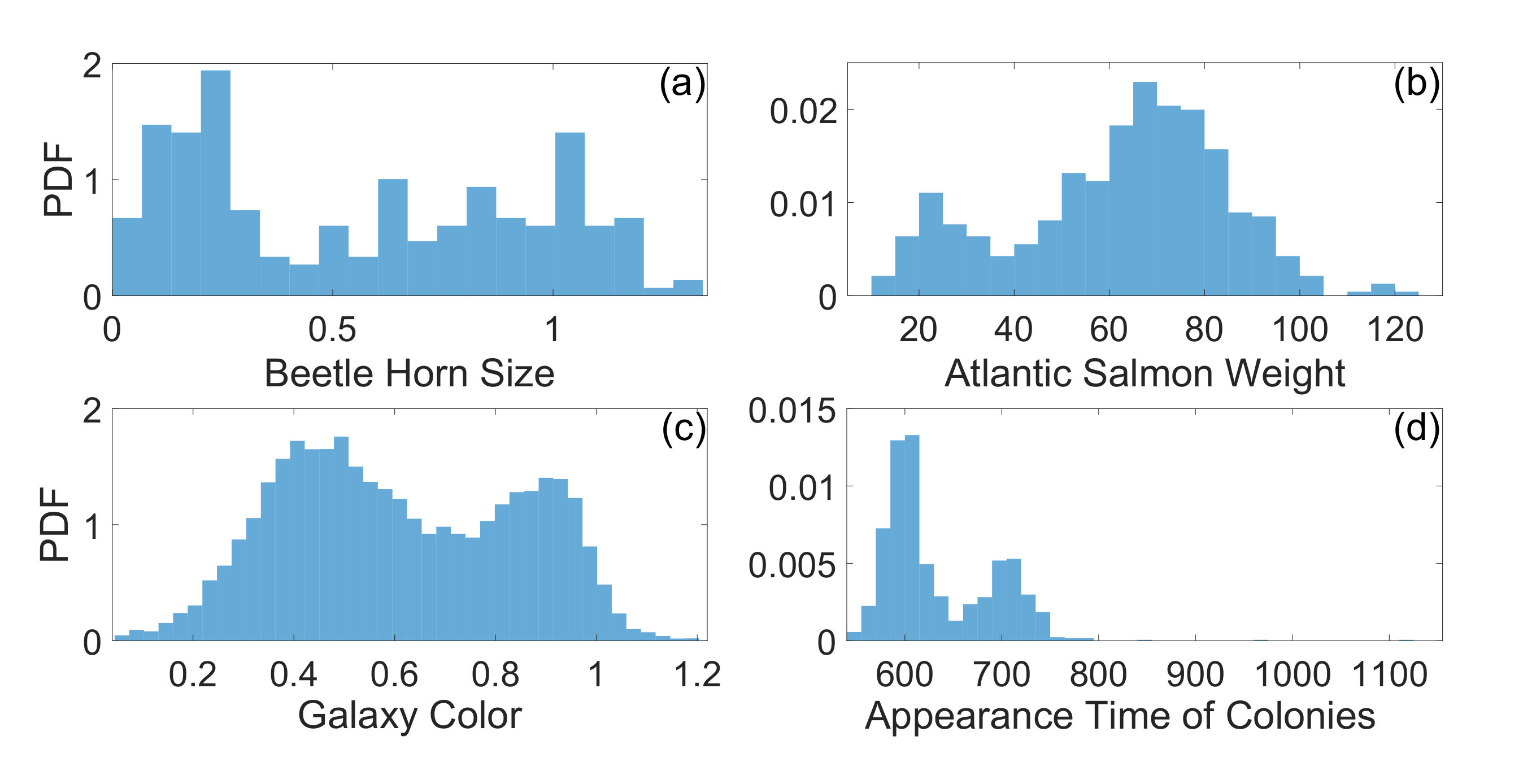 Figure 7
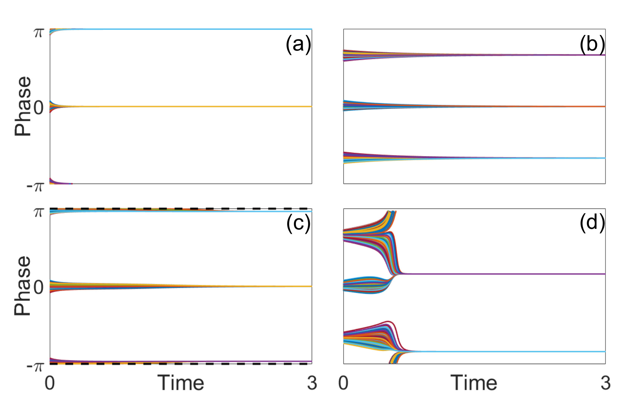 Figure 8
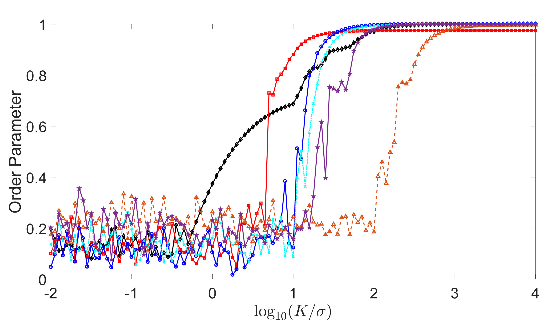 Figure 9
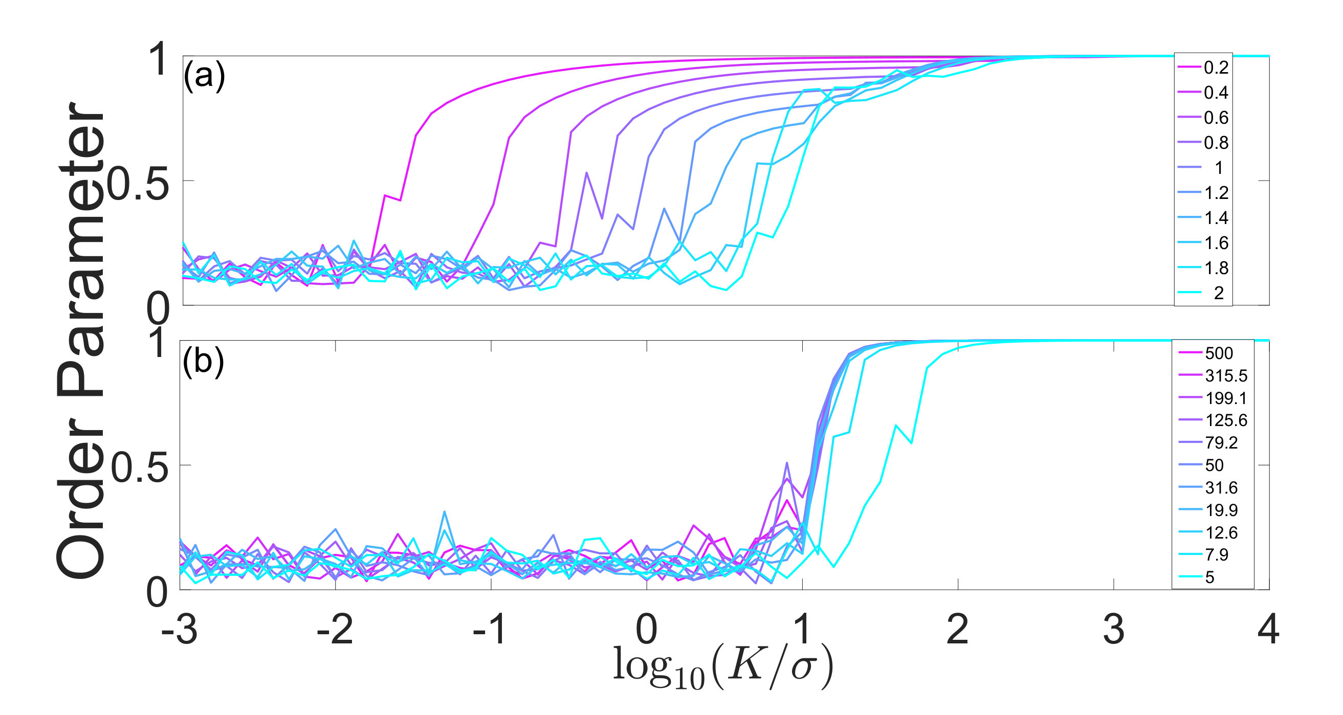 Figure 10
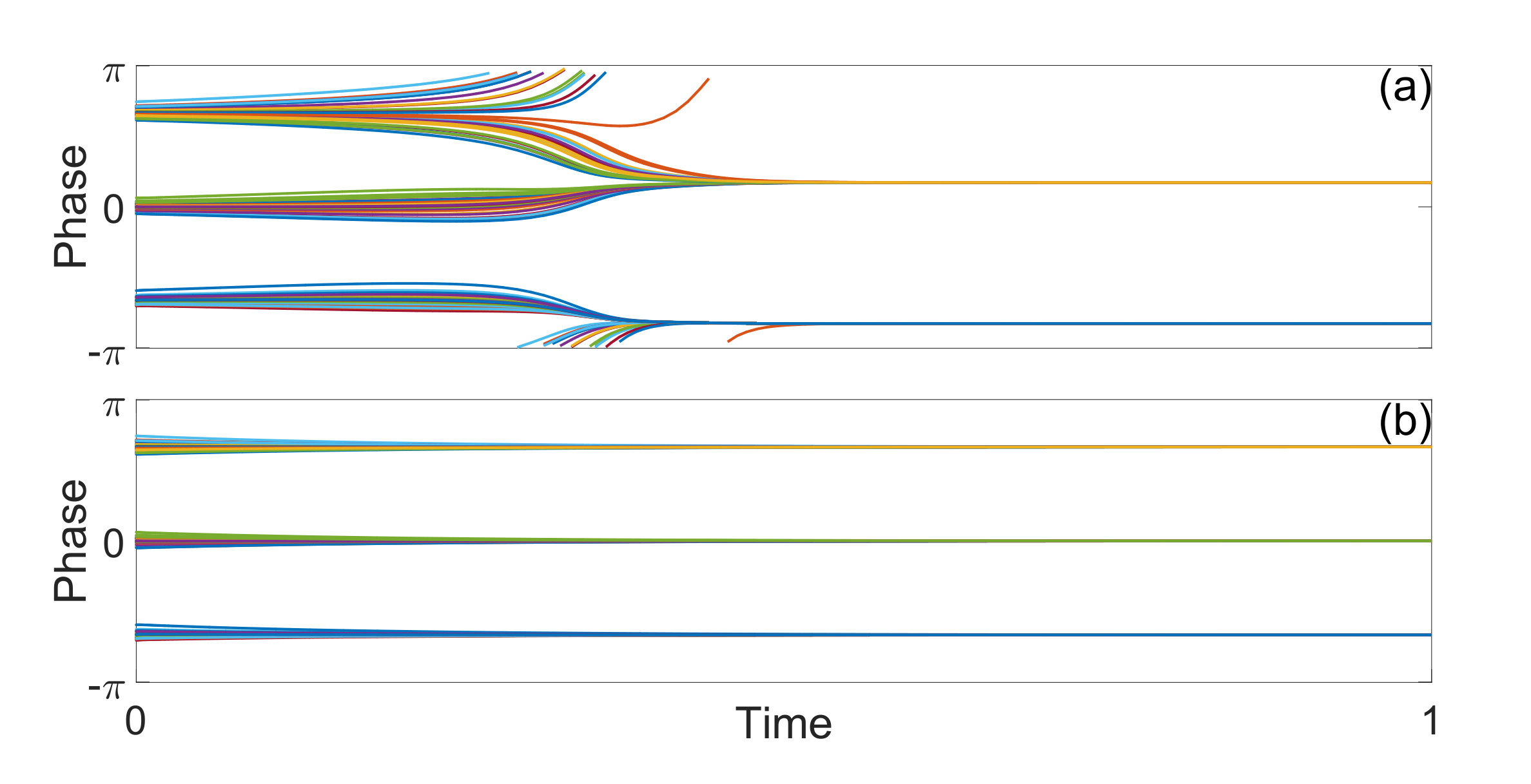 Figure 11
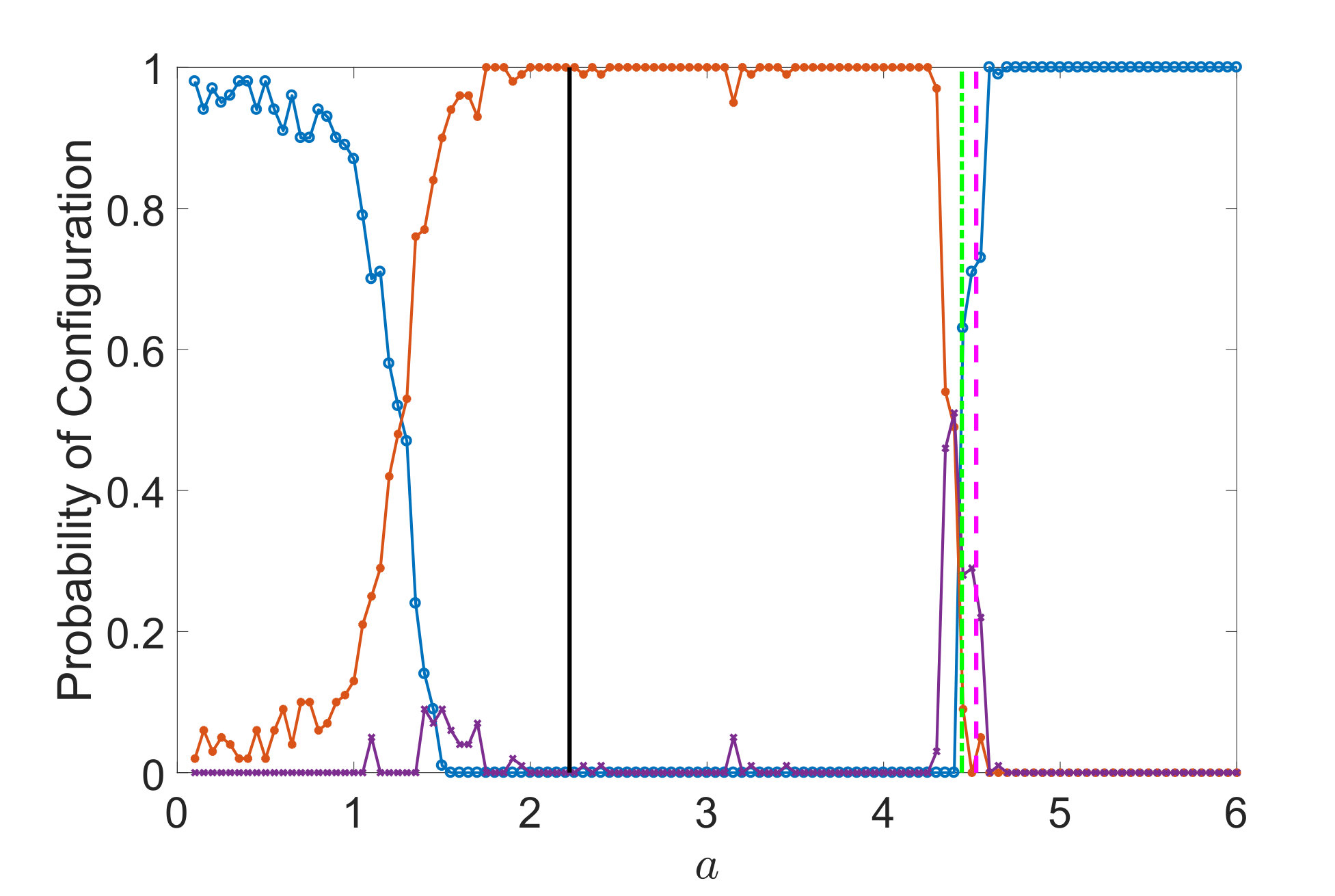 Figure 12
Peer Reviews
No public reviews on file for this paper yet. If you reviewed it on a platform where reviews are public (OpenReview, ICLR, NeurIPS, ICML), you can paste yours below so the community can read it here.
Videos
No videos yet. Explain this paper in a talk, walkthrough, or lecture? Add one.
\NewEnviron
scaletikzpicturetowidth[1]\BODY
A coupled oscillator model for the origin of bimodality and multimodality
J.D. Johnson
D.M. Abrams
Department of Engineering Sciences and Applied Mathematics, Northwestern University
McCormick School of Engineering and Applied Science
2145 Sheridan Road Evanston, IL 60208
Department of Engineering Sciences and Applied Mathematics, Northwestern University
McCormick School of Engineering and Applied Science
2145 Sheridan Road Evanston, IL 60208
Abstract
Perhaps because of the elegance of the central limit theorem, it is often assumed that distributions in nature will approach singly-peaked, unimodal shapes reminiscent of the Gaussian normal distribution. However, many systems behave differently, with variables following apparently bimodal or multimodal distributions. Here we argue that multimodality may emerge naturally as a result of repulsive or inhibitory coupling dynamics, and we show rigorously how it emerges for a broad class of coupling functions in variants of the paradigmatic Kuramoto model.
††preprint: AIP/123-QED††preprint: AIP/123-QED
In this paper we employ oscillators as a test system for understanding how bimodality—the splitting of oscillators into two rather than one cluster—may emerge as a result of coupling between interacting units. We present numerical and analytical results showing that repulsive coupling can lead to bimodality (or multimodality) for a wide range of detailed interaction dynamics.
I Introduction
Synchronization is a widespread phenomenon observed in biological Saigusa et al. (2008); Myung et al. (2015); Taylor et al. (2009), chemical Toiya et al. (2010); Vaidyanathan (2015); Li et al. (2003), physical Pantaleone (2002); Yoshida et al. (2000); Henk and Alejandro (2003); Ulrichs, Mann, and Parlitz (2009), and social settings Repp (2005); Kirschner and Tomasello (2009); De Paula (2009); Pluchino, Latora, and Rapisarda (2006). A paradigmatic mathematical model that can explain synchronization in many contexts is the Kuramoto model Kuramoto (2003, 1975); Strogatz (2000); Acebrón et al. (2005); Moreno and Pacheco (2004). Much work has been done on understanding the complex and surprising dynamics of the Kuramoto model and its variants, but the vast majority of that research focuses on the case of attractive coupling; here we are interested in the case where the coupling is repulsive.
Repulsive (or inhibitory) coupling is of physical interest as it arises frequently in the context of neuronal networks (e.g., see refs. Myung et al., 2015; Wang, Chen, and Perc, 2011), chemical interactions (e.g., refs. Toiya et al., 2010; Epstein, 1991; Hohmann, Kraus, and Schneider, 1998), and many other systems (see refs. Koseska et al., 2007; Ullner et al., 2007, 2008; Marvel, Strogatz, and Kleinberg, 2009; Laje and Mindlin, 2002; Balázsi et al., 2001). Some coupled oscillator models have examined repulsive coupling: Giver et al. developed a local variant of the Kuramoto model with repulsive coupling based on the interaction between water micro-droplets with reactants of the Belousov-Zhabotinsky reaction Giver, Jabeen, and Chakraborty (2011). Hong and Strogatz developed two variants of the Kuramoto model that involved mixes of positive and negative coupling Hong and Strogatz (2011, 2012).
The relationship between network structure and repulsive coupling has also been analyzed, with LevnajićLevnajić (2011, 2012) showing that, given the network coupling structure, many different phase configurations can arise. Recently, it has been shown that synchronization can arise in both repulsive and attractive coupling scenarios subject to common noise Pimenova et al. (2016); Nagai and Kori (2010); Gil, Kuramoto, and Mikhailov (2010); Gong et al. (2019). Gong et al.Gong et al. (2019), inspired by the work of Gil et al.Gil, Kuramoto, and Mikhailov (2010), studied instances where common noise can lead to clustering in the phase distribution of oscillators for repulsive coupling.
Nakamura et al.Nakamura, Tominaga, and Munakata (1994) investigated the effect of time-delayed nearest-neighbor coupling in the Kuramoto model and found that it could lead to the development of clustered states for both attractive and repulsive coupling. Mishra et al.Mishra et al. (2015) demonstrated that “chimeralike” states could arise with globally coupled Liénard systems incorporating both attractive and repulsive mean-field feedback. Yeldesbay et al.Yeldesbay, Pikovsky, and Rosenblum (2014) established that chimeralike states can arise in the Kuramoto-Sakaguchi model. They also considered a model with oscillators that could be synchronous (attractive coupling) or asynchronous (repulsive coupling) depending on their natural frequencies. They found that in this case a chimera state arises.
Golomb et al.Golomb et al. (1992) showed that clustering is possible in a coupled oscillator model with repulsive coupling that is suited for strong interactions between the limit-cycle oscillators. They further provided theory for when a frequency locked stationary phase distribution and when a nonperiodic attractor can arise.
Tsimring et al.Tsimring et al. (2005) showed that heterogeneous globally coupled oscillators obeying the standard Kuramoto model can cluster with all configurations having a zero order parameter, but this clustering breaks down as the number of oscillators increases. They also showed that, with local coupling, clustering can occur for nonidentical oscillators given sufficiently large coupling strength.
Closest to the work we present here, OkudaOkuda (1993) looked at the effect that an arbitrary coupling function may have on oscillators and developed theory as to when an -cluster state, with all clusters being the same size, can arise. He found that harmonics in the coupling function are necessary for clusters to arise.
The central limit theorem Billingsley (1995) may influence us to expect that distributions in nature should tend to a singly-peaked, unimodal shape akin to the Gaussian normal distribution. Yet, bimodality and multimodality can be observed in biological Chaudhary, Saeedi, and Costello (2016); Seeman et al. (1984a); Lewis and Rinzel (2003), social Wu et al. (2010a); DiMaggio, Evans, and Bryson (1996); Flay (1978), and chemical Bonifacio et al. (2015); Reiter and Epstein (1987); Ren-Chang, Jian-Chun, and Qiu-Jun (2011); Sun and Nesbitt (1977) contexts and beyondDekel and Birnboim (2006); Zhang, Mapes, and Soden (2003); Kuhl and Meltzoff (1982) (see Fig. 1 for selected examples). In this paper we demonstrate that multimodality may arise as a result of repulsive or inhibitory coupling dynamics and we give an in-depth explanation of how it can arise for a range of coupling functions.
II Model with antisymmetric repulsive coupling
We begin by considering a system of phase oscillators characterized by natural frequencies . The oscillators are globally coupled with coupling strength through an interaction function that depends only on the phase difference between each pair of oscillators:
[TABLE]
Here represents attractive coupling and represents repulsive coupling.
We consider interaction functions , , that satisfy the following conditions:
[TABLE]
These conditions impose: (2a) no coupling effects between oscillators in sync; (2b) locally attractive (repulsive) coupling near sync state for (); (2c) odd interaction function; (2d) no discontinuities in ; (2e) -periodic interaction function on domain. We point out that conditions and lead to .
II.1 Identical Oscillators
We assume that oscillators frequencies are drawn from a known frequency distribution . For simplicity we first consider the case of identical oscillators, i.e., we set the distribution to be , so the system becomes
[TABLE]
II.2 Bimodal equilibria
We assume that the number of oscillators is large, , and we look for bimodal equilibria by making the ansatz of an oscillator phase distribution , where describes the fraction in cluster 1. Note that this constitutes an explicit restriction to a bimodal manifold within the broader space of all possible oscillator phase distributions. Then system (3) can be reduced to two coupled ordinary differential equations (ODEs):
[TABLE]
We define a new phase-difference variable and write its dynamical system by subtracting Eq. (4) from Eq. (5):
[TABLE]
We observe that the fixed points of the system for are fully determined by the zeros of . From the assumptions above must have zeros at and . Furthermore, if conditions (2a–2e) hold and has no other zeros (as in the case of the red dashed curve from Fig. 2), then it is implied that . Hence, within the bimodal manifold, the fixed point at should be stable with being unstable. corresponds to a bimodal equilibrium with two clusters of oscillators separated by 180∘ of phase.
If additional roots of exist between [math] and , these will also correspond to bimodal fixed points with alternating stability (again restricted to the bimodal manifold). We focus on the cases where there are no other fixed points or there is exactly one other fixed point in ; other cases are similarly tractable. Figure 2 illustrates the typical general shapes of the interaction functions that we consider.
II.2.1 Stability of bimodal equilibrium
To investigate the broader stability of solutions to perturbations outside the bimodal manifold, we consider the perturbation of a single oscillator by a small amount . Because , we approximate the dynamics of the two clusters as unaffected by this perturbation. We examine the evolution of distance between the perturbed oscillator and the group from which it was perturbed, , to evaluate whether the system returns to its initial state.
For convenience, we move into a rotating frame by redefining , which is equivalent to setting . Without loss of generality we choose oscillator index from the cluster for the perturbation and assume , and thus (assuming for now that our interaction function has only one or zero fixed points in ). Then , and
[TABLE]
We expand the functions in a Taylor series to linear order:
[TABLE]
Assuming that (repulsive coupling, our case of interest in this manuscript), this implies stability if and only if
[TABLE]
A nearly identical calculation starting with the perturbation of a single oscillator from the (zero phase) cluster leads to a similar equation,
[TABLE]
Since Eqs. (7) and (8) must be simultaneously satisfied for stability of the full bimodal distribution, the following inequality must hold:
[TABLE]
Interestingly, this implies that the slope of the interaction function must be steeper at compared to if the bimodal state is to be stable. We can also compute explicit bounds on the proportion of the oscillators in each group by isolating fraction in inequality :
[TABLE]
III Concrete example
As a concrete example, we consider a simple class of interaction functions
[TABLE]
These functions have roots on at [math], , and , and satisfy all the conditions set forth earlier in section II. As long as there are three roots in , and one can check that for all choices of (see Fig. 3 for example plots). For inequality (10) to be satisfiable, we require
[TABLE]
which reduces to
[TABLE]
We note that symmetry of the roots allows us to consider positive without loss of generality. Figure 4 shows the results of numerical experiments where we test this predicted stability threshold. In each panel, Eq. (3) is implemented with the interaction function from Eq. (11). We initialize oscillators at and at , then add a small random perturbation to each oscillator’s initial phase, where is drawn from the normal distribution , with used in Fig. 4. We numerically integrate the system using a 4th/5th order Runge-Kutta scheme and consider evidence for stability if it approaches the unperturbed state, i.e. with . We note that in these experiments we set coupling strength .
In panels (a) and (b), we use oscillators, , and set , consistent with the stability threshold from Eq. (12), . The stable band of fractionation according to inequality (10) is then . In panel (a), we set , below the band’s upper bound; in panel (b), we set , above the band’s upper bound. As expected, the bimodal equilibrium appears stable in panel (a), but unstable in panel (b), where eleven oscillators move between clusters to establish a different equilibrium within the stable fractionation band ().
In panels (c) and (d), we again use oscillators and , but here we examine the predicted stability threshold from Eq. (12). We expect the bimodal state with to be unstable for all positive (but note that this state ceases to exist when ). We set since this is within the fractionation stability band from inequality (10) for all . In panel (c), we set , just below the threshold for stability; in panel (d), we set , just barely in the unstable domain. As expected, the bimodal equilibrium again appears stable in panel (c), but it appears unstable in panel (d). Since no fractionation will lead to a stable bimodal equilibrium, the system must move to an entirely different state, and it appears to converge to a trimodal distribution of oscillator phases.
We are able to understand why the system converges to a trimodal state by performing a similar analysis for the stability of three-cluster, or trimodal, oscillator distributions. One can show that a necessary condition for stability is:
[TABLE]
where is the angle separating clusters at and ( identified with ), and , , and are the fractionations of the three clusters at , , and respectively. With equal spacing between the clusters , the necessary condition simplifies to
[TABLE]
For the example function shown in Eq. (11) this is
[TABLE]
This implies that a trimodal state remains stable for all . It stably coexists with the bimodal state for , and may coexist with other multimodal states for . In general different multimodal states may stably coexist over various parameter ranges. More details of the analysis for trimodality can be found in the appendix.
IV Generalization to asymmetric interaction functions
We can relax assumption (2c) of an antisymmetric coupling function and still find stability boundaries for multimodal states. In place of Eq. (which used oddness of the coupling function), we find instead
[TABLE]
Clearly and both remain fixed points. Other fixed points exist if
[TABLE]
has a solution on . Figure 5 shows an example of an asymmetric interaction function. Geometrically this condition can be understood as identifying intersections of and its reflection when (or scaled versions when ). Once multimodal fixed points are identified, stability analysis is analogous to that presented earlier.
V Generalization to non-identical oscillators
We argue that real-world bimodal or multimodal distributions may result from similar dynamics to those presented in this paper. Of course, heterogeneity is inevitable in most real-world systems, yet we have focused thus far on the case of identical oscillators. While we leave the more general analysis for future work, we have conducted numerical experiments that appear to show that the predicted behavior occurs even in the presence of oscillator heterogeneity.
Again using the same example interaction function from Eq. (11), we now draw frequencies, , from a normal distribution and set the initial phases of the oscillators to (fraction ) or (fraction ), where is a small perturbation draw from the distribution . Figure 6 shows the results of perturbation experiments analogous to those presented in Fig. 4, with analogous results except that the final phase distributions have phases that cluster about the modes rather than all converging to them precisely (right panels show histograms of final states).
In Fig. 6 panels (a) and (b), we use oscillators and set and . Even with perturbed initial phases and heterogeneous natural frequencies, the oscillators still remain in the bimodal state as predicted for . Specifically, panel (b) shows that the steady state distribution of oscillators has finite-width clustering about the fixed point positions predicted from the identical-oscillator case. In panels (c) and (d), since , the bimodal state breaks down (consistent with the prediction of the identical-oscillator theory) and the system appears to converge to a trimodal equilibrium with three finite-width clusters.
VI Discussion
Coupled oscillators are an excellent testbed for models of synchronization or clustering. Even though real-world variables (e.g., sediment grain sizeSun et al. (2004), salmon body sizeThorpe (1977); Damsgrd et al. (2019), human communication frequencyWu et al. (2010b), dopamine receptor densitySeeman et al. (1984b), neutron star massSchwab, Podsiadlowski, and Rappaport (2010), galaxy colorBaldry et al. (2004), gamma ray burst durationMao, Narayan, and Piran (1994), tree heightEichhorn (2010), animal ornament sizeClifton, Braun, and Abrams (2016a)) may not be oscillatory or confined to a periodic domain, bimodality may emerge for qualitatively similar reasons. In our model, the coupling of one unit’s dynamical behavior to that of others is key to the phenomenon.
For clarity of presentation we have focused on a single example of interaction function (Eq. (11)), but evaluation of two other classes of interaction functions (triangle waves and antisymmetrized von-Mises kernels) also supports our analytical results—see supplementary material for details. In supplementary material, we also present further results regarding dependence of bimodal equilibria on coupling strength , as well as some numerical evidence regarding sizes of basins of attraction; each of these topics merits further in-depth study. The analysis we present here focuses exclusively on the case of all-to-all coupling; we leave further investigation of the impact of network structure for future work.
For real-world scenarios where bimodality or multimodality is of interest, the interaction function may not be known exactly. Nevertheless, we expect that it will often be possible to assess whether the conditions expressed in Eqns. (2) hold in a particular case. It also seems plausible that functions describing real-world interactions between coupled systems will have no more than a handful of roots, making bimodality and trimodality likely outcomes when repulsive or inhibitory coupling is imposed.
One particularly important case occurs when the interaction function has only roots at zero and , with the root at zero having larger or equal magnitude slope. That is the case in the standard Kuramoto model with sinusoidal coupling. In such a case we expect that the incoherent splay state will be stable. In general, the splay state should be stable when the tendency to cluster (due to long-distance interactions) cannot overcome the oscillators’ locally repulsive interactions.
VII Conclusions
We have shown that, when coupling is repulsive, multi-modality of the oscillator distribution can be a stable configuration for a wide range of interaction functions. We showed that bimodality can be expected under repulsive coupling when the slope of the interaction function at the origin is shallower than at the other root(s). We performed numerical experiments for both identical and nonidentical oscillators and observed results consistent with theory.
This demonstration that repulsive coupling can produce clustering under reasonable assumptions about the interaction dynamics is important as repulsive coupling is present in many natural systems. Hence, the theory we present in this paper provides an argument as to why one might expect multi-modality instead of unimodality or incoherence in systems known to have repulsive coupling.
Supplementary Material
See accompanying supplementary material for numerical experiments using a selection of additional interaction functions, for discussion of basins of attraction for different states, and for discussion of coupling strength dependency.
Appendix A Trimodal equilibria
We again consider a function that satisfies conditions (2a)–(2e). We look for solutions with oscillators distributed according to , where , so that the oscillators will be in three clusters at , , and (we again assume that the natural frequencies are identical):
[TABLE]
Here, . We define two variables and , so that the system reduces to
[TABLE]
We set , and arrive at the following system of equations:
[TABLE]
To set bounds on the fractionation of the clusters, we assume that there exists points such that Eqns. (21) and (22) are satisfied. Additionally, we put our system of coupled oscillators into a rotating frame so that . In the rotating frame, we set , , and . As before we perturb an oscillator from one of the three groups. We do this for all three groups and get a system of inequalities
[TABLE]
All these must be simultaneously satisfied for stability of a trimodal state. Adding, we find
[TABLE]
This states that the weighted sum of the slopes of the coupling function at , where the weights are the proportions for the groups separated by , is greater in magnitude than the slope at the origin. This condition reduces to
[TABLE]
if . As an example, we return to the class of interaction functions that we introduced in Section II. We relax the assumption that and consider the case when . To satisfy inequality , this means that
[TABLE]
which reduces to
[TABLE]
Figure 7 shows the results of a numerical experiment where we test this threshold. In both panels we use , , , and set . We expect the trimodal state to be unstable for . In panel (a) we set and perturb the oscillators by amount , with values drawn from the distribution . We can see that this perturbation leads to the system leaving the trimodal state and going to a bimodal state with phase difference.
One might be interested in why the bimodal state is stable in panel (a). Since there are only zeros at and , one may check the stability by evaluating the derivative of at these points. One can show that if
[TABLE]
the antiphase state is stable. Thus, when the trimodal state becomes unstable and perturbations lead to the stable bimodal state.
For the case, when , both the trimodal state and the bimodal state are stable configurations. Figure 8 shows the result of the numerical experiment where we place the parameter inside the previously stated interval and outside of the interval. In all panels we use , and set . As before, in all panels we perturb the oscillators by amount from the predicted fixed points, whose values are drawn from the distribution . In panels (a) and (b) we set . In these cases we expect both the bimodal state and the trimodal state to be stable for this value of . In panels (a) and (b), we set the fractionation to be equal in all groups, and we set the spacing between groups to be equal. As expected, we see that the trimodal state and the bimodal state are stable under perturbation.
In panel (c) we set . As expected, we see that the bimodal state is unstable and the system goes in to trimodal state. Given the proximity of the clusters to , we have added black dashed lines that at , so that one can see that the difference between the final state and . In panel (d), we set . We also observe an expected result, as trimodality appears to be unstable and the system converges to a bimodal equilibrium, which is stable given that .
In summary, we have a necessary condition for the stability of the trimodal equilibrium. Although, this condition is only necessary for stability, not sufficient, numerical experiments seems to point to it being an accurate threshold in examples we have considered. Also, theory and numerical experiments demonstrate that multistability of different multimodal equilibria is possible over parameter space. The theory for the stability of higher modes we leave for future work.
References
- Saigusa et al. (2008) T. Saigusa, A. Tero, T. Nakagaki, and Y. Kuramoto, Physical Review Letters 100, 018101 (2008).
- Myung et al. (2015) J. Myung, S. Hong, D. DeWoskin, E. De Schutter, D. B. Forger, and T. Takumi, Proceedings of the National Academy of Sciences 112, E3920 (2015).
- Taylor et al. (2009) A. F. Taylor, M. R. Tinsley, F. Wang, Z. Huang, and K. Showalter, Science 323, 614 (2009).
- Toiya et al. (2010) M. Toiya, H. O. González-Ochoa, V. K. Vanag, S. Fraden, and I. R. Epstein, The Journal of Physical Chemistry Letters 1, 1241 (2010).
- Vaidyanathan (2015) S. Vaidyanathan, International Journal of ChemTech Research 8, 759 (2015).
- Li et al. (2003) Y.-N. Li, L. Chen, Z.-S. Cai, and X.-Z. Zhao, Chaos, Solitons & Fractals 17, 699 (2003).
- Pantaleone (2002) J. Pantaleone, American Journal of Physics 70, 992 (2002).
- Yoshida et al. (2000) R. Yoshida, M. Tanaka, S. Onodera, T. Yamaguchi, and E. Kokufuta, The Journal of Physical Chemistry A 104, 7549 (2000).
- Henk and Alejandro (2003) N. Henk and R.-a. Alejandro, Synchronization of mechanical systems, Vol. 46 (World Scientific, 2003).
- Ulrichs, Mann, and Parlitz (2009) H. Ulrichs, A. Mann, and U. Parlitz, Chaos: An Interdisciplinary Journal of Nonlinear Science 19, 043120 (2009).
- Repp (2005) B. H. Repp, Psychonomic bulletin & review 12, 969 (2005).
- Kirschner and Tomasello (2009) S. Kirschner and M. Tomasello, Journal of Experimental Child Psychology 102, 299 (2009).
- De Paula (2009) A. De Paula, Journal of econometrics 148, 56 (2009).
- Pluchino, Latora, and Rapisarda (2006) A. Pluchino, V. Latora, and A. Rapisarda, The European Physical Journal B-Condensed Matter and Complex Systems 50, 169 (2006).
- Kuramoto (2003) Y. Kuramoto, Chemical oscillations, waves, and turbulence (Courier Corporation, 2003).
- Kuramoto (1975) Y. Kuramoto, in International symposium on mathematical problems in theoretical physics (Springer, 1975) pp. 420–422.
- Strogatz (2000) S. H. Strogatz, Physica D: Nonlinear Phenomena 143, 1 (2000).
- Acebrón et al. (2005) J. A. Acebrón, L. L. Bonilla, C. J. P. Vicente, F. Ritort, and R. Spigler, Reviews of modern physics 77, 137 (2005).
- Moreno and Pacheco (2004) Y. Moreno and A. F. Pacheco, EPL (Europhysics Letters) 68, 603 (2004).
- Wang, Chen, and Perc (2011) Q. Wang, G. Chen, and M. Perc, PLoS one 6, e15851 (2011).
- Epstein (1991) I. R. Epstein, Physica D: Nonlinear Phenomena 51, 152 (1991).
- Hohmann, Kraus, and Schneider (1998) W. Hohmann, M. Kraus, and F. Schneider, The Journal of Physical Chemistry A 102, 3103 (1998).
- Koseska et al. (2007) A. Koseska, E. Volkov, A. Zaikin, and J. Kurths, Physical Review E 75, 031916 (2007).
- Ullner et al. (2007) E. Ullner, A. Zaikin, E. I. Volkov, and J. García-Ojalvo, Physical review letters 99, 148103 (2007).
- Ullner et al. (2008) E. Ullner, A. Koseska, J. Kurths, E. Volkov, H. Kantz, and J. García-Ojalvo, Physical Review E 78, 031904 (2008).
- Marvel, Strogatz, and Kleinberg (2009) S. A. Marvel, S. H. Strogatz, and J. M. Kleinberg, Physical review letters 103, 198701 (2009).
- Laje and Mindlin (2002) R. Laje and G. B. Mindlin, Physical review letters 89, 288102 (2002).
- Balázsi et al. (2001) G. Balázsi, A. Cornell-Bell, A. B. Neiman, and F. Moss, Physical Review E 64, 041912 (2001).
- Giver, Jabeen, and Chakraborty (2011) M. Giver, Z. Jabeen, and B. Chakraborty, Physical Review E 83, 046206 (2011).
- Hong and Strogatz (2011) H. Hong and S. H. Strogatz, Physical Review Letters 106, 054102 (2011).
- Hong and Strogatz (2012) H. Hong and S. H. Strogatz, Physical Review E 85, 056210 (2012).
- Emlen (1996) D. J. Emlen, Evolution 50, 1219 (1996).
- Clifton, Braun, and Abrams (2016a) S. M. Clifton, R. I. Braun, and D. M. Abrams, Proceedings of the Royal Society B: Biological Sciences 283, 20161970 (2016a).
- Clifton, Braun, and Abrams (2016b) S. Clifton, R. Braun, and D. Abrams, Dryad Digital Repository.(doi: 10.5061/dryad. vb1pp) (2016b).
- Damsgrd et al. (2019) B. Damsgrd, T. H. Evensen, Ø. Øverli, M. Gorissen, L. O. Ebbesson, S. Rey, and E. Höglund, Royal Society Open Science 6, 181859 (2019).
- Damsgård et al. (2019) B. Damsgård, T. Evensen, Ø. Øverli, M. Gorissen, L. Ebbesson, S. Ray, and E. H’́aglund, “Data from: Proactive avoidance behaviour and pace-of-life syndrome in atlantic salmon,” (2019).
- Blanton et al. (2003) M. R. Blanton, D. W. Hogg, N. A. Bahcall, I. K. Baldry, J. Brinkmann, I. Csabai, D. Eisenstein, M. Fukugita, J. E. Gunn, Ž. Ivezić, et al., The Astrophysical Journal 594, 186 (2003).
- Abazajian et al. (2003) K. Abazajian, J. K. Adelman-McCarthy, M. A. Agüeros, S. S. Allam, S. F. Anderson, J. Annis, N. A. Bahcall, I. K. Baldry, S. Bastian, A. Berlind, et al., The Astronomical Journal 126, 2081 (2003).
- Baldry et al. (2004) I. K. Baldry, K. Glazebrook, J. Brinkmann, Ž. Ivezić, R. H. Lupton, R. C. Nichol, and A. S. Szalay, The Astrophysical Journal 600, 681 (2004).
- Ronin et al. (2017) I. Ronin, N. Katsowich, I. Rosenshine, and N. Q. Balaban, Elife 6, e19599 (2017).
- Goldberg et al. (2014) A. Goldberg, O. Fridman, I. Ronin, and N. Q. Balaban, Genome medicine 6, 112 (2014).
- Levnajić (2011) Z. Levnajić, Physical Review E 84, 016231 (2011).
- Levnajić (2012) Z. Levnajić, Scientific Reports 2, 967 (2012).
- Pimenova et al. (2016) A. V. Pimenova, D. S. Goldobin, M. Rosenblum, and A. Pikovsky, Scientific Reports 6, 38518 (2016).
- Nagai and Kori (2010) K. H. Nagai and H. Kori, Physical Review E 81, 065202 (2010).
- Gil, Kuramoto, and Mikhailov (2010) S. Gil, Y. Kuramoto, and A. S. Mikhailov, EPL (Europhysics Letters) 88, 60005 (2010).
- Gong et al. (2019) C. C. Gong, C. Zheng, R. Toenjes, and A. Pikovsky, Chaos: An Interdisciplinary Journal of Nonlinear Science 29, 033127 (2019).
- Nakamura, Tominaga, and Munakata (1994) Y. Nakamura, F. Tominaga, and T. Munakata, Physical Review E 49, 4849 (1994).
- Mishra et al. (2015) A. Mishra, C. Hens, M. Bose, P. K. Roy, and S. K. Dana, Physical Review E 92, 062920 (2015).
- Yeldesbay, Pikovsky, and Rosenblum (2014) A. Yeldesbay, A. Pikovsky, and M. Rosenblum, Physical review letters 112, 144103 (2014).
- Golomb et al. (1992) D. Golomb, D. Hansel, B. Shraiman, and H. Sompolinsky, Physical Review A 45, 3516 (1992).
- Tsimring et al. (2005) L. Tsimring, N. Rulkov, M. Larsen, and M. Gabbay, Physical Review Letters 95, 014101 (2005).
- Okuda (1993) K. Okuda, Physica D: Nonlinear Phenomena 63, 424 (1993).
- Billingsley (1995) P. Billingsley, Probability and Measure. 1995 (John Wiley & Sons, New York, 1995) p. 357.
- Chaudhary, Saeedi, and Costello (2016) C. Chaudhary, H. Saeedi, and M. J. Costello, Trends in Ecology & Evolution 31, 670 (2016).
- Seeman et al. (1984a) P. Seeman, C. Ulpian, C. Bergeron, P. Riederer, K. Jellinger, E. Gabriel, G. Reynolds, and W. Tourtellotte, Science 225, 728 (1984a).
- Lewis and Rinzel (2003) T. J. Lewis and J. Rinzel, Journal of Computational Neuroscience 14, 283 (2003).
- Wu et al. (2010a) Y. Wu, C. Zhou, J. Xiao, J. Kurths, and H. J. Schellnhuber, Proceedings of the National Academy of Sciences 107, 18803 (2010a).
- DiMaggio, Evans, and Bryson (1996) P. DiMaggio, J. Evans, and B. Bryson, American Journal of Sociology 102, 690 (1996).
- Flay (1978) B. R. Flay, Behavioral Science 23, 335 (1978).
- Bonifacio et al. (2015) P. Bonifacio, E. Caffau, M. Spite, M. Limongi, A. Chieffi, R. Klessen, P. François, P. Molaro, H.-G. Ludwig, S. Zaggia, et al., Astronomy & Astrophysics 579, A28 (2015).
- Reiter and Epstein (1987) J. Reiter and I. R. Epstein, Journal of Physical Chemistry 91, 4813 (1987).
- Ren-Chang, Jian-Chun, and Qiu-Jun (2011) Y. Ren-Chang, B. Jian-Chun, and F. Qiu-Jun, Atmospheric and Oceanic Science Letters 4, 229 (2011).
- Sun and Nesbitt (1977) S.-S. Sun and R. W. Nesbitt, Earth and Planetary Science Letters 35, 429 (1977).
- Dekel and Birnboim (2006) A. Dekel and Y. Birnboim, Monthly Notices of the Royal Astronomical Society 368, 2 (2006).
- Zhang, Mapes, and Soden (2003) C. Zhang, B. E. Mapes, and B. J. Soden, Quarterly Journal of the Royal Meteorological Society: A Journal of the Atmospheric Sciences, Applied Meteorology and Physical Oceanography 129, 2847 (2003).
- Kuhl and Meltzoff (1982) P. K. Kuhl and A. N. Meltzoff, Science 218, 1138 (1982).
- Sun et al. (2004) D. Sun, J. Bloemendal, D. K. Rea, Z. An, J. Vandenberghe, H. Lu, R. Su, and T. Liu, Catena 55, 325 (2004).
- Thorpe (1977) J. Thorpe, Journal of Fish Biology 11, 175 (1977).
- Wu et al. (2010b) Y. Wu, C. Zhou, J. Xiao, J. Kurths, and H. J. Schellnhuber, Proceedings of the National Academy of Sciences 107, 18803 (2010b).
- Seeman et al. (1984b) P. Seeman, C. Ulpian, C. Bergeron, P. Riederer, K. Jellinger, E. Gabriel, G. Reynolds, and W. Tourtellotte, Science 225, 728 (1984b).
- Schwab, Podsiadlowski, and Rappaport (2010) J. Schwab, P. Podsiadlowski, and S. Rappaport, The Astrophysical Journal 719, 722 (2010).
- Mao, Narayan, and Piran (1994) S. Mao, R. Narayan, and T. Piran, The Astrophysical Journal 420, 171 (1994).
- Eichhorn (2010) M. Eichhorn, Journal of forest research 15, 391 (2010).
Supplementary Material: A coupled oscillator model for the origin of bimodality and multimodality
J.D. Johnson D.M. Abrams
Supplementary Material: A coupled oscillator model for the origin of bimodality and multimodality
Appendix S1 Additional Coupling Functions
Figure S1 illustrates two additional coupling functions that we examined. We used a variant of the triangle wave (blue, solid) given by the equation
[TABLE]
assuming that , and an antisymmetrized variant of the von Mises distribution (red curves) given by
[TABLE]
We numerically probe the stability of the bimodal equilibrium using these interaction functions in Fig. S2. Here , the oscillators’ frequencies are drawn from a distribution , the phase perturbation, , is drawn from the distribution and we set . In panels (a) and (b) we take the triangle wave defined in Eq. (S29) and set ; this gives a stable fractionation threshold . We test that threshold numerically by setting in panel (a) and in panel (b). As expected, we see that the fractionation is stable in panel (a) and is unstable in panel (b).
In panels (c) and (d) we use the antisymmetrized von-Mises function from Eq. (S30) with and . In panel (c) we set , and, as expected, we see that the bimodal equilibrium appears unstable; this is because there does not exist a range of such that Eq. (10) can be satisfied given that the slope at the origin is far steeper than the slope at the . We note that in (c) the system appears to tend to the incoherent state. In panel (d) we set and observe that the bimodal state appears to be stable under perturbation, which is expected given that the slope at the is steeper when compared to the origin.
Appendix S2 Basins of Attraction for Multimodal States
We have conducted some preliminary numerical exploration of the sizes of basins of attraction for various equilibria for the example interaction function given in Eq. (11) of the main text. We simulated the system one hundred times with initial phases chosen independently at random from the uniform distribution over the circle, i.e. , and evaluated the fraction of the time that the system converged to each distinct equilibrium state. Results are shown in Fig. S3, with , , and oscillator natural frequencies drawn from the distribution .
Fig. S3 also shows the stability thresholds described in Eqns. (12) (bimodal state), (A.13) (antiphase state), and trimodal state (A.12) of the main text, visualized by the solid black, and dot-dashed green, and magenta vertical lines respectively. In order to classify the observed equilibria, we use a -means algorithm on the unit circle, with the number of clusters, , being decided by the gap statistic. We say that a equilibrium state is bimodal if , trimodal if , and so on.
We note that the results are consistent with our analysis in that the probability of a configuration is always zero in ranges of where it is excluded. Although, we have not analyzed equilibria with more than three modes, we observe that such modes are unlikely to be observed for most values of , and thus have apparently small basins of attraction.
Given that this experiment was conducted with heterogeneous oscillators, this lends plausibility to the idea that the system will end up in a multimodal state for sufficiently large coupling. More formal analysis of the basin size of the bimodal and trimodal state will be left for future work.
Appendix S3 Critical Coupling Strength
In the standard Kuramoto model with attractive coupling, there exists a critical coupling strength at which the system bifurcates from an incoherent state to the ordered state. To look for dependence in the system detailed in main text, we examine the simplest cases of and , and also conduct several numerical experiments with results shown in Fig. S4, though we leave more thorough exploration for future work.
Figure S4 shows how order varies as we increase coupling strength among nonidentical oscillators with the concrete interaction function used in the main text. Here, we set and draw the frequencies from the distribution . From here, we vary the quantity so that runs from -2 to 4. Each curves shown above represents the result of an experiment for a given value of . Here, the order parameter is defined as follows:
[TABLE]
Defining the order parameter in this fashion sets the value of the order parameter to be 1 whenever the final configuration is bimodal or an equally spaced trimodal solution. Just as in the standard Kuramoto model, if the coupling strength is not sufficiently large in magnitude, the system goes to the incoherent state due to intrinsic oscillator heterogeneity. We observe that the critical coupling strength appears to be proportional to the standard deviation of the frequency distribution, similar to the result in the standard Kuramoto analysis, but we point out that the critical coupling strength also appears to have dependence on the value of . We believe that some insight into this dependence can be gained from examining the simple and cases, though more rigorous analysis is left for future work.
For , the system reduces to
[TABLE]
where . Setting , we find that a fixed point must satisfy the equation:
[TABLE]
Note, this fixed point does not always exist, but if the coupling function has zeros, a fixed point must arise as .
Even without explicitly defining , we can observe scaling dependencies for the critical coupling strength , which is defined such that
[TABLE]
where is the value such that (the arg max). We observe that , which is expected if as in the standard Kuramoto model (since for two oscillators ) and is observed in our numerical experiments even for .
We also observe that scales with the maximum value of the interaction function , which in our numerical experiments depends on the parameter . Similar dependence is also evident if we consider the case.
For , we take the natural frequencies (without loss of generality) to be respectively. As before, we convert to difference coordinates and , and arrive at two conditions for existence of equilibria:
[TABLE]
which simplify to
[TABLE]
Hence, a necessary condition must satisfy for the existence of equilibria is
[TABLE]
So, just as in the case, we see that the critical coupling strength is proportional to the oscillator heterogeneity and inversely proportional to the maximum of the interaction function .
We hypothesize that similar scaling laws hold for , and find that such a hypothesis is consistent with data from numerical experiments shown in Fig. S4.
The reference list from the paper itself. Each links out to its DOI / PubMed record.
- 1Saigusa et al. (2008) T. Saigusa, A. Tero, T. Nakagaki, and Y. Kuramoto, Physical Review Letters 100 , 018101 (2008).
- 2Myung et al. (2015) J. Myung, S. Hong, D. De Woskin, E. De Schutter, D. B. Forger, and T. Takumi, Proceedings of the National Academy of Sciences 112 , E 3920 (2015).
- 3Taylor et al. (2009) A. F. Taylor, M. R. Tinsley, F. Wang, Z. Huang, and K. Showalter, Science 323 , 614 (2009).
- 4Toiya et al. (2010) M. Toiya, H. O. González-Ochoa, V. K. Vanag, S. Fraden, and I. R. Epstein, The Journal of Physical Chemistry Letters 1 , 1241 (2010).
- 5Vaidyanathan (2015) S. Vaidyanathan, International Journal of Chem Tech Research 8 , 759 (2015).
- 6Li et al. (2003) Y.-N. Li, L. Chen, Z.-S. Cai, and X.-Z. Zhao, Chaos, Solitons & Fractals 17 , 699 (2003).
- 7Pantaleone (2002) J. Pantaleone, American Journal of Physics 70 , 992 (2002).
- 8Yoshida et al. (2000) R. Yoshida, M. Tanaka, S. Onodera, T. Yamaguchi, and E. Kokufuta, The Journal of Physical Chemistry A 104 , 7549 (2000).