Refined swampland distance conjecture and exotic hybrid Calabi-Yaus
David Erkinger, Johanna Knapp

TL;DR
This paper tests the refined swampland distance conjecture in the Kahler moduli space of exotic Calabi-Yaus, confirming its validity through explicit geodesic length computations using sphere partition functions.
Contribution
It provides the first explicit verification of the refined swampland distance conjecture in exotic Calabi-Yau examples with pseudo-hybrid points, including non-abelian gauge models.
Findings
Refined swampland distance conjecture holds at pseudo-hybrid points.
Explicit geodesic length calculations confirm theoretical predictions.
Sphere partition function effectively computes Kahler metric in these models.
Abstract
We test the refined swampland distance conjecture in the Kahler moduli space of exotic one-parameter Calabi-Yaus. We focus on examples with pseudo-hybrid points. These points, whose properties are not well-understood, are at finite distance in the moduli space. We explicitly compute the lengths of geodesics from such points to the large volume regime and show that the refined swampland distance conjecture holds. To compute the metric we use the sphere partition function of the gauged linear sigma model. We discuss several examples in detail, including one example associated to a gauged linear sigma model with non-abelian gauge group.
Click any figure to enlarge with its caption.
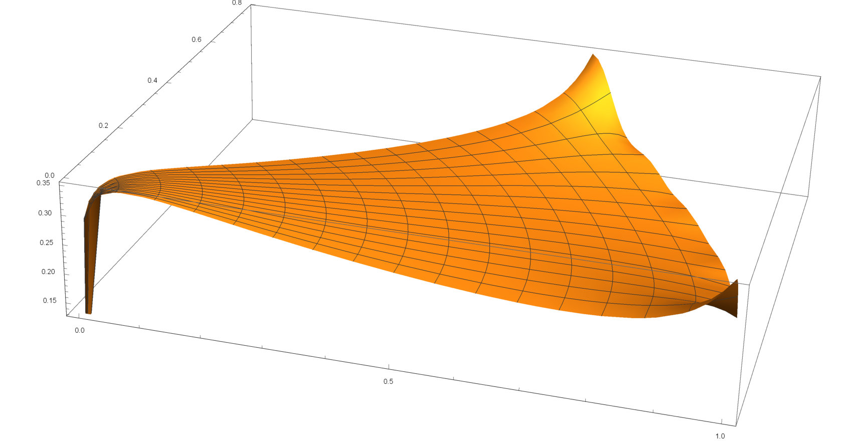 Figure 1
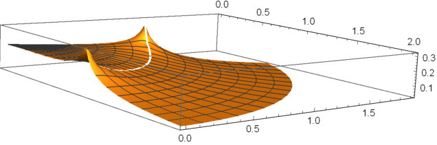 Figure 2
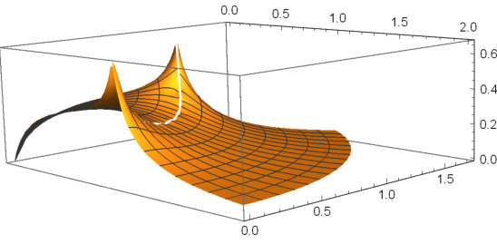 Figure 3
 Figure 4
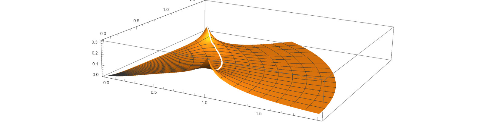 Figure 5
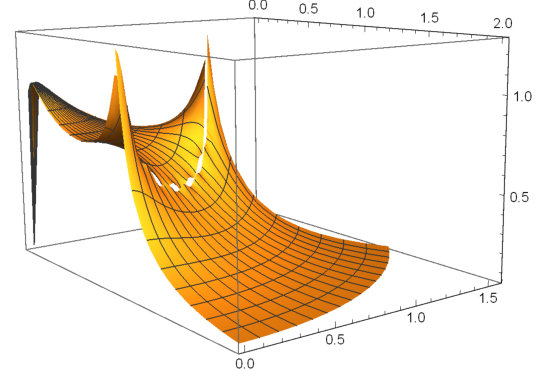 Figure 6
| type | distance on | description | |
|---|---|---|---|
| finite | Landau-Ginzburg, pseudo-hybrid | ||
| finite | (mirror of) conifold, pseudo-hybrid | ||
| infinite | hybrid | ||
| infinite | geometric |
| label | at | |||
|---|---|---|---|---|
| C1 | ||||
| C2 | ||||
| C3 |
| label | : | at | (sing. at ) | ||
|---|---|---|---|---|---|
| F1 | |||||
| F2 | |||||
| F3 |
| 1 | 2 | 3 | 4 | 5 | |
|---|---|---|---|---|---|
| 6 | 7 | 7 | 9 | 10 | |
Peer Reviews
No public reviews on file for this paper yet. If you reviewed it on a platform where reviews are public (OpenReview, ICLR, NeurIPS, ICML), you can paste yours below so the community can read it here.
Videos
No videos yet. Explain this paper in a talk, walkthrough, or lecture? Add one.
UWThPh2019-14
Refined swampland distance conjecture and exotic hybrid Calabi-Yaus
David [email protected], Johanna [email protected]
*Mathematical Physics Group, University of Vienna
Boltzmanngasse 5, 1090 Vienna, Austria*
Abstract
We test the refined swampland distance conjecture in the Kähler moduli space of exotic one-parameter Calabi-Yaus. We focus on examples with pseudo-hybrid points. These points, whose properties are not well-understood, are at finite distance in the moduli space. We explicitly compute the lengths of geodesics from such points to the large volume regime and show that the refined swampland distance conjecture holds. To compute the metric we use the sphere partition function of the gauged linear sigma model. We discuss several examples in detail, including one example associated to a gauged linear sigma model with non-abelian gauge group.
Contents
- 1 Introduction
- 2 Refined swampland distance conjecture
- 3 GLSM and sphere partition function
- 4 Models with
- 5 Testing the refined swampland distance conjecture
- 6 Conclusions
- A Evaluating the sphere partition function
- B Transforming the leading metric behavior
1 Introduction
Initiated by [1, 2], there has been tremendous activity around the question of how to characterize consistent UV complete theories of quantum gravity, referred to as the landscape, as opposed to the swampland which encompasses all theories that do not have this property. This has led to a whole zoo of swampland conjectures based upon which one can decide whether a given theory of quantum gravity is in the landscape or in the swampland. A recent review of the state-of-the-art, including hundreds of references, can be found in [3].
As string theory is believed to be a consistent theory of quantum gravity, any low-energy effective theory that comes from string theory should be part of the landscape. In the landscape of Calabi-Yau (CY) compactifications, those corners corresponding to large volume regions are the most studied. The inspiration for many conjectures comes from the typical properties of string theory at large volume. Considering regions in the moduli space that are far away from large volume points provides a non-trivial test for the validity of the conjectures. In this work we aim to test one of the conjectures in more exotic corners of the stringy moduli space.
Concretely, we will test the refined swampland distance conjecture (RSDC) [4, 5, 6]. The swampland distance conjecture (SDC) was first proposed in [2] and states that at infinite distance from a given point in the moduli space the effective theory breaks down because an infinite tower of light states appears. The information that enters these conjectures can be readily obtained from standard techniques in string theory and has been tested in concrete settings [7, 8, 9, 10, 11, 12, 13, 14, 15, 16, 17, 18, 19]. The refined swampland distance conjecture was proposed in [4, 5, 6]. It gives a bound on the lengths of geodesics in the scalar moduli space of a theory of quantum gravity. In [20, 21] the conjecture was tested by computing the lengths of geodesics in the Kähler moduli space of CY threefolds. This was done by explicitly calculating the (quantum corrected) metric on and numerically solving the geodesic equation in order to determine the lengths of the geodesics. In particular it was shown that geodesics starting at Landau-Ginzburg points, i.e. limiting points at finite distance in the moduli space, and going all the way to a large volume point satisfy the RSDC. The main examples were CY hypersurfaces with one and two parameters.
The goal of this work is to extend the discussion of [20] to one-parameter CYs that are more exotic. Our focus will be on examples of CYs that have pseudo-hybrid points. Pseudo-hybrid models [22] are, like Landau-Ginzburg models, at finite distance in the moduli space, but their field theoretic description is not well-understood. They have been linked to singular CFTs, and it has been argued that they do not have a proper limit where gravity decouples. Due to these somewhat mysterious properties, they make good candidates for testing the RSDC. For this purpose we will compute lengths of geodesics from such points to large volume points.
In order to compute the metric on the moduli space we use the gauged linear sigma model (GLSM) [23] and supersymmetric localization. In [24, 25] it was shown that the sphere partition function [26, 27] of the GLSM computes the exact Kähler potential on . This method allows us to compute the metric directly on without taking the detour to the complex structure moduli space of the mirror. Furthermore, by means of supersymmetric localization one can access all regions of and is not restricted to well-studied large volume settings. Another advantage is that these methods also apply for CYs associated to non-abelian GLSMs. Such CYs cannot be analyzed within the framework of toric geometry. One of our examples will be a one-parameter CY with a pseudo-hybrid point that arises from a GLSM with non-abelian gauge group [28].
The article is organized as follows. In section 2 we recall the swampland distance conjecture and its refinement and discuss how it is realized for Kähler moduli spaces of CYs. Section 3 provides a lightning review on GLSMs and the sphere partition function. In section 4 we discuss our examples and give some details on the properties of pseudo-hybrids from the viewpoint of the GLSM. We then proceed to compute the sphere partition function. The main results of the article are presented in section 5 where we test the RSDC for our examples. We confirm the conjecture holds for these exotic models.
While this work was in preparation [15] appeared which also computes the metrics on for the examples we discuss, albeit with different methods.
Acknowledgments: We would like to thank Ralph Blumenhagen, Emanuel Scheidegger, Thorsten Schimannek, Eric Sharpe and Harald Skarke for discussions and comments on the manuscript. JK thanks the University of Chicago for hospitality. The authors were supported by the Austrian Science Fund (FWF): [P30904-N27]. JK was also supported by a faculty grant of the Universities of Chicago and Vienna.
2 Refined swampland distance conjecture
The swampland distance conjecture (SDC) is a statement on the properties of the scalar moduli spaces of a consistent theory of quantum gravity. The claim is that, given a scalar moduli space and a point , there exist other points that are arbitrarily far away from . At these parametrically large distances an infinitely large tower of light states appears,
[TABLE]
where and are the masses at and , respectively. The geodesic distance is obtained from the metric on . As the field theory description breaks down due to infinitely many massless degrees of freedom.
In [5, 20] a refined swampland distance conjecture (RSDC) was put forward. It gives constraints on the parameter in (2.1). Define and denote by the geodesic distance from at which the exponential drop-off sets in. Then the RSDC states that, in Planck units,
[TABLE]
In this work we will test the RSDC in a concrete setting and collect further evidence in its favor. To this end, we choose a framework where also the inspiration for many of these conjectures comes from: type II string compactifications on compact CY threefolds. We consider the parameter space to be the Kähler moduli space of the CY.
In such settings one can test the conjecture by explicitly computing lengths of geodesics in . This is not a trivial task, because the stringy Kähler moduli space decomposes into chambers, not all of which contain large volume points. Generic paths on will cross boundaries between chambers. This amounts to analytic continuation beyond the range of validity of a choice of local coordinates on . Thus, the computation of the geodesic distances between two generic points and crossing various chambers in has to be split up into computing geodesics within the individual chambers that are matched along the boundaries. According to the RSDC, one expects that all the distances involved are of order .
The Kähler moduli space of a CY is itself a Kähler manifold. To obtain the metric, one computes the Kähler potential on , where are the Kähler moduli. Given , the metric is
[TABLE]
The Kähler potential is subject to worldsheet instanton corrections. To compute it, one can either use mirror symmetry or results from supersymmetric localization [26, 27, 24, 25]. The latter link the Kähler potential to the sphere partition function of the GLSM associated to the CY. We will use the GLSM method. The necessary ingredients will be summarized in section 3.
Once one has the Kähler metric, one can compute the distance between two points and in the same chamber via
[TABLE]
where is an affine parameter. If we take into account quantum corrections to comparatively high orders, it is hard to evaluate this integral analytically. Instead, the geodesics can be obtained by numerically solving the geodesic equation
[TABLE]
In the following, we will restrict ourselves to models with . It is convenient to express the complex coordinate in terms of radial and an angular variable, i.e. in (2.5). In these coordinates, the geodesic equation becomes
[TABLE]
Given suitable starting values, these equations can be solved numerically in order to obtain the lengths of the geodesics. In the examples we have considered we solved the geodesic equation up to order . Given these results, we can explicitly evaluate the distances in (2.2). We start from a point at finite distance in a certain chamber in and then cross the boundary of the chamber to approach a point at infinite distance. The exponential drop-off becomes significant in the second chamber after traversing a path of length . Therefore, is the proper distance from the starting point to the chamber boundary, and the distance after which the tower of light states appears in the chamber with a limiting point at infinite distance. The full length of the geodesic is then characterized by [20]
[TABLE]
Conjecturally, this is also of order . In section 5 we will test the RSDC for such examples.
3 GLSM and sphere partition function
To define an GLSM we choose a (not necessarily abelian) gauge group . The scalar components of the chiral multiplets are coordinates on a vector space . They transform in the matter representation . In the general case one has . For the CY case the matter representation must satisfy . This translates into the condition that the weights () of , i.e. the gauge charges of the matter fields, sum to zero. Furthermore there is a vector R-symmetry under which the fields transform in the representation . GLSMs associated to compact CYs have a non-zero superpotential , which has R-charge . Let and be the Lie algebras of and of a maximal torus , respectively. The scalar components of the gauge multiplet are denoted by . We further denote the FI parameters and the (-periodic) theta angles by , respectively. For the calculations using the sphere partition function it is convenient to define . This FI-theta parameter is related to the complexified Kähler parameter of the CY. We further define a pairing . With , there are natural pairings and .
To determine the vacua of the theory one has to find the zeros of the scalar potential
[TABLE]
where is the moment map and is the gauge coupling. The first term implies which we will assume from now on. Among the solutions to , there are two special classes. The first one is which implies
[TABLE]
The first expression are the D-term equations, the second the F-terms. There can be different solutions depending on the values of . These are referred to as phases of the GLSM. They divide up the parameter space, and hence , into chambers. In this way GLSMs can be used to probe the stringy Kähler moduli space. In the phases some or all of the gauge symmetry is broken. If a continuous subgroup is unbroken, one has a strongly coupled phase, otherwise one refers to the phases as Higgs phases.
Another type of solutions are those where for all . Then the theory develops a Coulomb branch. Classically, this can only happen if some of the FI parameters are zero, i.e. at phase boundaries. The gauge group is broken to the maximal torus , and the are unconstrained. The Coulomb branch is lifted by one-loop corrections which generate an effective potential for :
[TABLE]
The first term is the classical term, are the positive roots of . The Coulomb branch persists at the critical locus of . Via mirror symmetry this locus maps to part of the discriminant in the complex structure moduli of the mirror CY. In models with more than one Kähler modulus there are also mixed branches. Since we will not discuss such models in this work, we refrain from giving details. When computing geodesics, one should avoid the singular loci encoded in .
For the computation of the Kähler potential we use the sphere partition function . This was first computed in [26, 27] via supersymmetric localization. The connection to was first observed in [24]:
[TABLE]
The definition of the sphere partition function for the CY case is
[TABLE]
where is a normalization constant. The integral can be evaluated using the residue theorem. Depending on the phase, entering via in the exponential, one closes the contours such that one gets a convergent expression. In models with non-abelian , these are multidimensional integrals even if .
4 Models with
In this section we will discuss examples of CYs with one Kähler parameter and their associated GLSMs. The GLSMs have two phases, i.e. the stringy Kähler moduli space is divided into two chambers. Along the boundary between two phases there are singular points where the theory has a Coulomb branch. We will mainly focus on geodesics that cross the phase boundary.
The limiting points in the phases and at the phase boundaries of one-parameter models can be characterized by the local exponents () associated to each point. These exponents are determined by the Picard-Fuchs operator related to the CY. To be precise, the Picard-Fuchs operator is usually associated to the mirror CY where is a local coordinate in the complex structure moduli space of the mirror. However, it has been shown that also the sphere and the hemisphere partition function of the GLSM satisfy GKZ and Picard-Fuchs equations [29, 30, 31]. Therefore it makes sense to associate differential operators to phases of GLSMs.
Consider the Picard-Fuchs differential operator , where is the local coordinate around the singular point at . The exponents are determined by solving
[TABLE]
Picard-Fuchs operators of this type have been constructed systematically [32]. Depending on the structure of , the corresponding points in have been referred to as -, -, -, and -points in [32, 15]. Their properties are summarized in table 1.
-points are at finite distance in the moduli space. Typical examples are Landau-Ginzburg orbifold theories, but they can also correspond to more exotic phases that have properties similar to Landau-Ginzburg models. -points are also at finite distance. These points arise at the singular points at the phase boundaries, but can also appear as limiting points in a phase. The latter case has been studied for instance in [22, 33], where models of this type were named pseudo-hybrids. -points are at infinite distance in the moduli space, and it has been argued in [15] that an infinite number of D-branes becomes massless, as expected by the SDC. -points typically correspond to hybrid phases, which are described in terms of Landau-Ginzburg orbifolds fibered over some base manifold. Finally, -points are also at infinite distance. These are geometric points, as one finds them in large volume phases. In the one-parameter case, the RSDC has been shown to hold for geodesics connecting Landau-Ginzburg and -points [20]. In this work we will discuss geodesics from -points and other examples of -points to -points.
Let us give some more details on those -points that are the limiting points in pseudo-hybrid phases. We will characterize pseudo-hybrid phases by their common features. In all the known examples the classical vacuum in the pseudo-hybrid phase has more than one component. The different components exhibit different symmetry breaking patterns. In contrast to large volume or Landau-Ginzburg phases, a low energy effective description is currently unknown for pseudo-hybrid models. In [22] it was argued that such models may not have a proper limit where gravity decouples. The associated conformal field theories are singular. Another feature of these phases is that a finite number of branes become massless at the limiting point. Note that in the context of complete intersection CYs also certain -points can exhibit pseudo-hybrid behavior in the sense that the vacuum configurations have several branches associated to different Landau-Ginzburg models.
In the next three subsections we will introduce the examples we will be working with. We will recall the GLSM description and the discussion of the phases. We will first focus on abelian GLSMs with gauge group . There are models corresponding to CYs whose associated Picard-Fuchs operators are hypergeometric differential equations. See for instance [34, 35] for partial list and [36] for a full classification. The complete list has also recently been given in [15]. Three models within this class have -type pseudo-hybrid phases, see table 2. The first example was considered from a GLSM point of view in [22]. We also discuss the other two models. Furthermore we consider an -type example which is not a standard Landau-Ginzburg model. Finally, we also discuss a -type pseudo-hybrid phase of a non-abelian GLSM, first constructed in [28].
4.1 -type pseudo-hybrid examples from abelian GLSMs
In the following we will discuss three abelian GLSMs with a -type pseudo-hybrid phase. In table 2 we collect some information on these examples, including the geometry in the large volume () phase, the Hodge numbers, and the local exponent in the pseudo-hybrid phase at . For further information see also [15].
4.1.1 C1
The GLSM of this model was discussed in [22] and we repeat the GLSM analysis here. The chiral matter content is
[TABLE]
The gauge invariant superpotential is
[TABLE]
where are generic homogeneous polynomials of degrees , respectively. The D-term equation is
[TABLE]
where is the FI parameter. The F-terms are
[TABLE]
In the phase we find a smooth complete intersection of codimension in as indicated in table 2:
[TABLE]
The exotic phase is at . The D-term excludes the point and the F-terms imply that . Thus, the classical vacuum is a weighted . To see the full picture, we have to turn on classical fluctuations of the . First we observe that for generic loci in we do not find proper vacua. In this case the gauge symmetry is completely broken. The Landau-Ginzburg model fibered over this base does not lead to a well-defined ground state. The superpotential contains quadratic terms, and hence all the are massive. Thus, we get zero contribution to the central charge, which implies that these vacua are not CY. Furthermore R-symmetry is broken: if all get a VEV and thus must have R-charge zero, there is no consistent way to assign R-charge to the such that the Landau-Ginzburg superpotential has R-charge two.
There are two special loci on the vacuum manifold which exhibit different behavior. At the point there is an unbroken , and one recovers a Landau-Ginzburg orbifold with superpotential in . There are no quadratic terms in the superpotential, and therefore all are massless. The R-symmetry is preserved: we can assign charge to all . This amounts to choosing in the table of charges above. The central charge of this Landau-Ginzburg model is , and we do not get a superconformal field theory of a CY. This implies that this Landau-Ginzburg model alone cannot describe the theory at low energies.
A further branch is a curve , where a is preserved and all can be assigned R-charge . This corresponds to in the table above. Fibering a Landau-Ginzburg orbifold over this curve, the superpotential is quadratic. Naively, one would assume that there are only massive degrees of freedom that do not play a role in the low-energy CFT. Also the R-charge assignment would indicate this. However, the situation is more subtle. Note that we can rewrite the Landau-Ginzburg potential as
[TABLE]
where is a generic matrix, linear in . When the rank of drops, i.e. when there will be massless degrees of freedom. This is a situation similar to the models studied in [37, 38].
To summarize, the -phase has two branches where the gauge symmetry is broken to a and a , respectively. The former is of a hybrid-type, the latter is a Landau-Ginzburg orbifold. This is the typical behavior of a pseudo-hybrid model.
Since we are interested in computing geodesics that cross phase boundaries we also have to determine the singularities at the phase boundaries that are encoded in the Coulomb branch of the GLSM. Given the scalar component of the vector multiplet, the effective potential is
[TABLE]
The critical locus is at
[TABLE]
Now we compute the sphere partition function in the two phases. Inserting into the definition (3.5) gives
[TABLE]
Applying the transformation
[TABLE]
we get
[TABLE]
To evaluate the sphere partition function in a given phase we close the integration contour in such a way that the integral converges. One has to take into account the poles of the Gamma functions that are enclosed in the contour. For details of this rather technical discussion we refer to appendix A.
In the phase we close the contour to the right so that only the poles coming from contribute. We obtain the following result:
[TABLE]
where
[TABLE]
and
[TABLE]
The evaluation of the sphere partition function in the phase is more involved. Closing the contour to the left, two types of poles of and contribute. Due to coinciding poles we have to be mindful not to over-count. There are two possibilities, namely a pole of is a simultaneous pole of and vice versa. A careful analysis reveals that whenever this happens the denominator of cancels such a contribution. Taking this into account, the sphere partition function is a sum of two terms. Again, we refer to the appendix for details. The total result is
[TABLE]
where
[TABLE]
with
[TABLE]
The second contribution is
[TABLE]
with
[TABLE]
4.1.2 C2
In this model the field content of the GLSM is
[TABLE]
The superpotential is
[TABLE]
where are generic polynomials of degrees and , respectively. In the phase we recover
[TABLE]
This complete intersection CY has Hodge numbers .
The phase is a pseudo-hybrid. The scalar potential is zero for and , which does not lead to well-defined vacua for generic . At the point one finds a Landau-Ginzburg orbifold with in . The R-charge assignment is as above with . This actually gives a CFT of central charge , i.e. it is CY. There is another branch with where a is preserved and the R-charges are given by . This theory is massive and one is tempted to argue that it does not contribute in the IR. Nevertheless, this branch seems to have some effect, because the limiting point is -point, as is reflected in behavior of computed below. It would be interesting to understand this better.
The Coulomb branch analysis shows that the singular point is at
[TABLE]
After the transformation (4.11) the sphere partition function is given by
[TABLE]
The evaluation of the partition function is similar to the C1-case. Therefore we will simply state the results in the two phases.
For on the poles of in (4.25) contribute and we obtain
[TABLE]
with
[TABLE]
The steps to obtain the result in the phase are the same as for the previous example. Again, we find two contributions from and :
[TABLE]
However, in contrast to the previous example we now have to take into account a possible over-counting of poles. Details on this issue are given in section A.2. From the poles of we get the following contributions:
[TABLE]
with
[TABLE]
From the poles of we get
[TABLE]
with
[TABLE]
4.1.3 C3
As the final example of this class we consider the GLSM with the following field content
[TABLE]
The superpotential is
[TABLE]
with generic polynomials of degrees and , respectively. The phase is again a complete intersection
[TABLE]
with Hodge numbers . The other phase is a pseudo-hybrid. The classical potential is zero for and . At one finds a Landau-Ginzburg orbifold in with potential , massive , and R-charge assignment . Curiously, the central charge of the CFT is , which exceeds the value for the CY case. There is another branch with with an unbroken and R-charges given by . The locus of the singularity is
[TABLE]
After the transformation (4.11) the sphere partition function reads
[TABLE]
The evaluation in the different phases can be done by the same methods as in the previous models and therefore we give only the final results in the two phases. The only subtlety is that now also in the phase two different poles contribute and we must take into account a potential over-counting. This is similar to the situation for the model in section 4.1.2 and therefore can be treated in the same way as outlined in section A.2.
In the phase we find that the only contribution is given by coinciding poles of and :
[TABLE]
with
[TABLE]
For we again find two contributions:
[TABLE]
with
[TABLE]
The second contribution is given by:
[TABLE]
and
[TABLE]
Closer inspection reveals that the poles cancel except for .
4.2 -type examples from abelian GLSMs
Among the hypergeometric examples there are three with limiting points of type that do not correspond to Landau-Ginzburg points. Earlier discussions of these examples can be found in [35, 39, 40, 41, 15]. We collect the relevant information about these models in table 3.
We describe them in terms of GLSMs with field content
[TABLE]
where the and can be read off from table 3. The superpotential has the form
[TABLE]
with homogeneous polynomials of degrees . The phases are the complete intersections indicated in table 3. The vacuum manifold in the -phase is . At the point there is an unbroken and one finds a corresponding Landau-Ginzburg orbifold at this point with a R-charge assignment for the fields. Analogously, one finds a Landau-Ginzburg orbifold at . The singular point in the moduli space and the corresponding values for can be read off from the last column in table 3.
Since these models are very similar to the -type models, we only compute the sphere partition function for one of them, namely F1. The definition of the sphere partition function for this case is
[TABLE]
where we have defined via (4.11) as usual. The evaluation in the -phase is completely analogous to the -type examples. The result is
[TABLE]
with
[TABLE]
In the -phase only first order poles contribute. This is a typical behavior for -type models. A study of the location of the poles reveals that certain poles of are a subset of the poles of . Therefore we will first take into account all poles of and then consider the remaining poles of . We find for the contribution:
[TABLE]
We see that only gives a non-zero contribution. The contributions for get canceled. This is anticipated as we expect only first order poles in this phase. Since we only have first order poles, the residue can be evaluated explicitly. We find
[TABLE]
with
[TABLE]
The contribution from results in:
[TABLE]
Again we only have first order poles and the result for the residue is
[TABLE]
with
[TABLE]
We have excluded the case as this would lead to a double counting of poles. Nevertheless this contribution would have been canceled anyway.
4.3 Non-abelian example with a pseudo-hybrid phases
So far, we have only discussed models that can be realized in terms of toric geometry and thus by abelian GLSMs. All the methods that we have used also apply to non-abelian GLSMs. Indeed, -type pseudo-hybrid phases also appear for non-abelian models. The first one-parameter example with a pseudo-hybrid phase was found in [28]. Further examples with have been identified in [42].
Due to conceptual and technical challenges, non-abelian models are difficult to come by. One problem is that one of the phases is typically strongly coupled, i.e. in the low-energy effective theory a continuous subgroup of the GLSM gauge group is unbroken. While it is understood how to compute the sphere partition function in such cases, the result will not be absolutely convergent, and one needs to apply Borel summation to get a convergent expression. In practice, this is doable only for the very lowest orders in the expansion. Another problem is related to the fact that all known one-parameter non-abelian GLSMs have more than one singular point at the phase boundary. This also means that the associated Picard-Fuchs differential operators are no longer hypergeometric. In the region between the singular points it is not clear whether one should choose the metric for the -phase or for the -phase. Neither will have good convergence properties there. A further complication is related to numerics. The expressions for the sphere partition function are more complicated than in the abelian case. This also complicates the numerical calculation of the geodesics. One aspect is that the calculations work much more efficiently for a suitable choice of coordinate on . As has been demonstrated in [20] for the abelian examples, it is best to choose a coordinate in such a way that the (only) singular point at the phase boundary is at . Having more than one singular point, there is no obvious choice for a “good” coordinate.
In view of these difficulties, we have not been able to give a complete discussion of geodesics crossing phase boundaries. Nevertheless, we have been able to make some explicit computations by restricting ourselves to geodesics within a weakly-coupled pseudo-hybrid phase. The example we consider is a one-parameter non-abelian GLSM with gauge group that has been discussed in [28]. The matter content is
[TABLE]
where refers to the fundamental representation and is the determinantal representation of . The superpotential is
[TABLE]
where (). By gauge invariance, the antisymmetric matrix has the following structure. The first block transforms according to , i.e. it is cubic in and bilinear in . The lower block transforms in the representation, which means that the entries are linear in . The off-diagonal blocks are in representation, i.e. the entries are quadratic in and linear in .
This model has an -point in the -phase which is a smooth Pfaffian CY in weighted [43] characterized by the condition . It is a strongly coupled phase where an subgroup of remains unbroken. The -phase is a pseudo-hybrid phase of type that is at finite distance in the moduli space.
There are two singular points at
[TABLE]
Note that the points are not at the same theta angle: and ().
The sphere partition function for this model has been computed in [28]. In our limited discussion we will compute the lengths of geodesics starting at the pseudo-hybrid point and ending at the -value of the nearest singular point. For this purpose we only need the result of the sphere partition function in the phase. The sphere partition function can be written as
[TABLE]
where we have defined () and . The contributions to the integrand are
[TABLE]
In the -phase the sphere partition function can be written as
[TABLE]
The first term is
[TABLE]
with
[TABLE]
The second contribution is
[TABLE]
where
[TABLE]
To obtain this result, one has to compute a multi-dimensional residue, which is considerably harder that the one-dimensional case that we had to deal with for the abelian GLSMs. Prescriptions for evaluating such integrals can be found for instance in [44, 45, 46, 47]. We outline some of the steps in appendix A.3. The leading behavior of the sphere partition function is [28]
[TABLE]
This is the expected behavior for a pseudo-hybrid phase.
5 Testing the refined swampland distance conjecture
In this section we present our results for the lengths of geodesics in the models discussed in section 4.
5.1 -type pseudo-hybrid examples from abelian GLSMs
5.1.1 C1
In section 4.1.1 we have computed the sphere partition function for this model. For the numerical calculations it is convenient to replace the variable by
[TABLE]
Furthermore, we write in terms of polar coordinates111We parameterize using the “classical” Kähler parameter with . Since our focus is on computing geodesic distances, the results will be independent of the choice of parametrization. We choose the one that seems most natural for the GLSM point of view. If we were to extract Gromov-Witten invariants from , we would have to follow the steps outlined in [24].:
[TABLE]
With this choice, the pseudo-hybrid point is at and the singular point at the phase boundary is at . Using this and the results eqs. 4.13, 4.17 and 4.19 of the sphere partition function, the leading behavior of the metric in the two phases is
[TABLE]
We plot the metric in fig. 1, along with the metric of the quintic.
As for the quintic, the limiting point at is at finite distance in the moduli space, but the behavior is slightly different due to the logarithm: near the singular point the logarithm dominates and the behavior of the metric is similar to a large volume phase. Near the pseudo-hybrid point the polynomial behavior wins over so that the distance remains finite. This is shown in fig. 2. We only see a divergent behavior if the geodesic ends at the singular point at the phase boundary (solid line). From the plot one can also read off at which value of the dependence on the angular variable sets in.
We are interested in computing geodesics that start near the pseudo-hybrid point and go all the way to the large volume phase. We call the distance inside the phase and calculate this distance as the geodesic distance to the phase boundary. In order to get an approximation for the distance behavior in the phase we follow the discussion of [20]. Looking at the leading behavior of the metric in phase and calculating the distance for a path with constant one gets:
[TABLE]
Replacing by gives:
[TABLE]
We also define as in (2.8). We compute the geodesics for various starting values for . As a starting value for we choose222Due to numerical issues we could not start at . The additional distance one should add by starting away from [math] turns out to be negligible. . Fitting against the asymptotic behavior, we get the values for the parameters that are summarized in table 4. The angular variable takes values between , but as one can see from the plot of the metric in fig. 1, there is a symmetry around . For the fit we therefore focus on the region . Let us also comment on the geodesics with small values of . These geodesics are rather short in the large radius phase and they are not very useful for testing the conjecture. Nevertheless we kept them in our discussion, because we are mostly interested in the behavior in the small radius regime. There they display no behavior which would justify an exclusion. The mean values of the fitted parameters are
[TABLE]
Our results are in agreement with the RSDC. Comparing to the quintic [20], we see that the numerical values of are by about a factor larger.
5.1.2 C2
The analysis of this model is completely analogous to the first one. Using the results of the sphere partition function from section 4.1.2, we define
[TABLE]
and further
[TABLE]
This parametrization moves the singularity to . The leading behavior of the metric in the two phases is
[TABLE]
A plot of the metric is given in fig. 3.
The plot in fig. 4 shows at which value of the angle dependence sets in.
The asymptotic behavior is the same as in (5.4), and so we can write:
[TABLE]
A table with the fitted values for this model is given in table 5.
Again we used the symmetry of the metric and focused on the region . Also in this model we started from . The mean values of the fitted parameters are
[TABLE]
This is again in agreement with the RSDC.
5.1.3 C3
Using the results of section 4.1.3 we define
[TABLE]
and
[TABLE]
This choice moves the singularity to . In these coordinates the leading behavior of the metric in the two phases is
[TABLE]
The metric has been plotted in fig. 3. As in the previous two examples, we compute the lengths of geodesics in the numerically,whereby as before we started from , and fit the geodesics in the phase against,
[TABLE]
The results are summarized in table 6. The mean values of the fitted parameters are
[TABLE]
which is in agreement with the RSDC.
5.1.4 Comparing C1, C2 and C3
Comparing the results for the distances in the pseudo-hybrid phase (see eqs. 5.6, 5.11 and 5.16), we see that the values vary between the models. These differences can be explained by looking at the asymptotic behavior of the metric333This has also been computed [15]. In appendix appendix B we transform our results to the form given in [15]. eqs. 5.3, 5.9 and 5.14. If we approach the point the contribution is strongly suppressed by the polynomial behavior in the models C2 and C3. For the model C1 the logarithmic contribution is only suppressed by and therefore we obtain the longest distance for these models. This behavior can also be seen in the plots of the metric figs. 3 and 1 and in more detail in the plots figs. 2 and 4 where we plotted the metric behavior in the pseudo-hybrid phase for different values of . One sees that in the C1 model the logarithmic behavior is much more dominant than for the other two models.
Comparing our results to the results given in [20] for the one parameter hypersurface examples we see that the C1 model shows the greatest deviations from the values given there. This can also be traced back to the different behavior of the metric in the pseudo-hybrid phase compared to the behavior of the metric in the Landau-Ginzburg phase of these models (see e.g. fig. 1 for the quintic). Models with Landau-Ginzburg phases yield much smaller values for than models with pseudo-hybrid phases. Among the pseudo-hybrid models, grows larger the more the metric of the model deviates from the metric in a Landau-Ginzburg phase. The specifics of the phase are thus related to the values of the distance. Based on these considerations, it seems possible to make more precise statements on the bounds (2.2).
The lengths associated to the large volume phases have a behavior comparable to the results of [20]. Whether the underlying geometry is a hypersurface or a complete intersection does not seem to have an obvious effect on the distance parameters.
5.2 -type example
The next example has been discussed in section 4.2. We choose the coordinate such that
[TABLE]
Given this, we define
[TABLE]
The remaining steps are the same as for the -type model. We plot the metric in fig. 5. Even though is singular at , the distance remains finite. This can be seen considering the leading order behavior of the metric in this phase:
[TABLE]
Integrating using (2.4) gives a finite contribution also for . The leading behavior in the large radius phase is the same as in the other models.
Plots of the metric for fixed values of are depicted in fig. 6.
Due to the symmetry in we consider geodesics for . Computing geodesics starting near444The starting value for the numerical calculation is . Using (2.4) one can compute the distance from to this value for a path with constant . One finds a contribution of which we added as a correction to the numerical results for . and ending in the -phase, we can numerically determine the length parameters as summarized in table 7. The mean values are
[TABLE]
We see that compared to the previous models, the distance in the -phase is larger than in the models C2 and C3 and larger than in the -type models discussed in [20]. The corresponding distance in the C1-model is slightly bigger. This behavior is as expected. This is illustrated in fig. 7, where we plotted the metric in the various model for the central value. Though the metric in the F1-model diverges at the origin, it soon drops significantly under the value of the metric in the C1-model. In total, we again find agreement with the RSDC.
5.3 Non-abelian example with a pseudo-hybrid phase
Based on the results of section 4.3, we can compute the distances for geodesics that start at the pseudo-hybrid point and end at the -value of the nearest singular point. Given (4.62), we find
[TABLE]
This means that is closer to the pseudo-hybrid phase. In order to simplify the calculation we introduce a coordinate in such a way that the pseudo-hybrid point is at and the nearest singular point is at . Following [43] it is convenient to choose
[TABLE]
Switching to polar coordinates, we define
[TABLE]
This moves the nearest singularity to .
The leading behavior of the metric is
[TABLE]
with
[TABLE]
We observe that the leading behavior is similar to the behavior of the C1-example, except for the prefactor . This also gives us an additional check for the distances we compute numerically. Compared to C1, they should scale with a factor . Note that , so the distances will be shorter than for C1.
The metric is plotted in fig. 8.
As for the abelian models we observe a symmetry around . To see where the -dependence sets in, we plot the metric for specific values of in fig. 9.
The numerical results for the distances for various starting values of are summarized in table 8.
The mean value of the distance in the pseudo-hybrid phase is
[TABLE]
This is in agreement with the RSDC. Comparing to the C1-model, we find that
[TABLE]
This is in good agreement with .
One can also get an approximation for by computing the integral (2.4) for the leading term of the metric, which is independent of . In this case we find . This is significantly smaller than (5.26). We can trace this back to the fact that we are integrating up to the boundary of the convergence radius at where the subleading terms give larger contributions555Of course the result is still convergent.. If we only integrate up to, say, the leading term is a good approximation.
6 Conclusions
In this work we have shown that the RSDC holds for exotic hybrid CYs. We did this by explicitly computing the lengths of geodesics in the Kähler moduli space of one-parameter CY threefolds with pseudo-hybrid phases, and confirmed the RSDC. The specifics of the model were reflected in the numerical values for the distances. There are several interesting directions for further research.
One of them concerns CYs arising as phases of non-abelian GLSMs. While we have seen indications that the RSDC is satisfied for these models, the discussion is certainly not fully satisfactory and should be improved by addressing the challenges discussed in section 4.3. We may return to this question in future work. In general, it might be worthwhile to study CYs that are not complete intersections in toric varieties in the context of swampland conjectures. A greater variety of examples might also improve the conjectures. For instance, one might be able to specify what “” means more precisely. It would be interesting to study in more detail how the properties of the phases influence the numerical values of the lengths of the geodesics. A similar observation has been made in [20] where it was observed that the lengths are related to the number of moduli.
Another interesting question concerns the SDC for exotic limiting points such as hybrid points that are at infinite distance in the moduli space. For -type hybrid models it has been conjectured in [15] that in infinite tower of D0 and D2-branes becomes massless. It would be interesting to understand this better, for instance with the help of the GLSM.
Finally, it may be interesting to further study the pseudo-hybrid phases themselves in more detail. In this work we were mainly concerned with testing the RSDC and did not require the details about the low-energy description of the - and -points. Nevertheless, our rather superficial discussion revealed some curious properties. In order to understand this better, a discussion of the other -type models along the lines of [22] that also includes an analysis of the behavior of D-branes in these phases may be worthwhile. Even though they look simpler, a thorough analysis of the -type examples may also be of interest. In this work we wrote down the most obvious abelian GLSMs for these models and obtained consistent results. As far as their construction in toric geometry is concerned, these models arise in a non-trivial way from models with more than one parameter [40, 41]. It would be interesting to understand these connections better via the GLSM.
Appendix A Evaluating the sphere partition function
Since we are only dealing with one-parameter models, the evaluation of the sphere partition function is relatively straight forward. See for instance [48] for a pedagogical discussion of a one-parameter example. We will discuss the details in a manner similar to [46] that also works for higher dimensional residue integrals.
The general form of a contribution in the sphere partition function from a matter field is
[TABLE]
The -function has poles if the argument takes values in . The expression (A.1) has poles in the numerator and the denominator:
[TABLE]
for .
The problem of the finding contributing poles can be recast into the geometric problem by introducing divisors. For a general contribution we get:
[TABLE]
In the one-dimensional case, i.e. for , we can simply solve to find the location of a pole:
[TABLE]
We also have to take into account possible cancellations of a pole of the numerator by a pole of the denominator in (A.1). To derive the conditions for when this happens we insert into and find
[TABLE]
Since a valid has to be in , we find the condition
[TABLE]
for a cancellation. As a consequence, the zeros of are only contributing poles if
[TABLE]
A.1 C1
Let us now give the details of the evaluation of the sphere partition function of the pseudo-hybrid model discussed in section 4.1. Our starting point is (4.12). The divisors for the pseudo-hybrid model, together with the conditions to avoid a cancellation are
[TABLE]
for . The poles lie along the real line, and we define the half-lines
[TABLE]
The exact location of the poles can be calculated from eqs. A.8, A.9 and A.10 and results in
[TABLE]
For , one finds
[TABLE]
First, we consider the phase, where the poles along , i.e. those coming from , contribute. Introducing a shift , one can write all the contributions in terms of residues at . The integrand of the sphere partition function becomes
[TABLE]
where we have introduced . To further simplify the calculation we define . This simplifies the sums:
[TABLE]
Further using the reflection formula , the terms in the integrand can be written as
[TABLE]
Putting everything together, we arrive at the result in the main text.
Next, we consider the phase, where the poles along contribute. Closing the contour to the left, two types of poles of and contribute. Due to cancellations of poles, we have to be mindful not to over-count. There are two possibilities, namely a pole of is a simultaneous pole of and vice versa. A careful analysis reveals whenever this happens the denominator of cancels such a contribution.
Let us first focus on the contribution from . We shift the integration variable so that . The contributions to the integrand become
[TABLE]
To simplify the summations we introduce which gives the sums
[TABLE]
Note the constraint on the sums in and which is solved by
[TABLE]
Hence, we introduce
[TABLE]
so that we finally arrive at
[TABLE]
The integrand of the sphere partition function becomes
[TABLE]
Applying the reflection formula as in the phase, we arrive at the result in the main text.
Finally, we consider the contribution of . Defining , the integrand can be written as
[TABLE]
The sum in is restricted to . Defining , the sums simplify to
[TABLE]
To remove the constraint on we further define
[TABLE]
which yields
[TABLE]
After these transformations the contributions to the integrand become
[TABLE]
Using the reflection formula the contribution to the sphere partition function becomes
[TABLE]
with
[TABLE]
Further investigation shows that only for there is a second order pole, for there is a cancellation of poles. Taking this into account, we finally arrive at the result in the main text.
A.2 C2
Here we will give details on the evaluation of the sphere partition function for the model discussed in section 4.1.2. As most of the steps are similar to the evaluation described in section A.1 we will only comment on the steps on how to avoid an over-counting of the poles. In this model an over-counting can only occur in the phase. This is obvious from the structure of the partition function (4.25). Therefore we will only discuss this phase.
The contributions in the small radius phase come from and . Similar to the steps in section A.1 we introduce the following divisors:
[TABLE]
The poles lie at
[TABLE]
Now one inserts a pole of into (A.33) and solves for . This gives
[TABLE]
A valid must fulfill . So it follows that poles coincide if:
[TABLE]
Similarly, by inserting a pole of into (A.32) and solving for for , one gets . This is expected, considering (A.39). We know that and we see that every pole of is a pole of . In order to avoid an over-counting we do the following. First we sum over all poles of and get so all poles of and the odd poles of . Then we sum over the even poles of and get the remaining poles of and avoid a double counting of poles of .
As for the evaluation in section A.1 we will reduce the integral to a sum over residues. Let us start with the contribution from . We make the following transformation:
[TABLE]
In this case the sums read
[TABLE]
To simplify the summation let us introduce . We get the constraint . From this it follows that
[TABLE]
Therefore we introduce
[TABLE]
This yields the following sums
[TABLE]
After all the transformations the integral contributions read:
[TABLE]
Putting everything together we find the result in section 4.1.2.
The contribution from is a little more involved, because we have to consider a restriction on the poles in order to avoid an over-counting. First we apply the transformation:
[TABLE]
Here we must restrict the sum to even , because the odd values are already accounted for in . Therefore we make the replacement . This results in the following sums
[TABLE]
where we introduced . But since we must impose . In order to fulfill this condition we set
[TABLE]
Due to we see that only are allowed contributions. So we get the following sums
[TABLE]
After these transformations the various contributions read
[TABLE]
Collecting all the results we get the expression in the main text.
We refrain from giving details on the evaluation of the sphere partition function in the model C3, because the discussion is completely analogous to C1 and C2. The same also holds for the model F1.
A.3 Non-abelian model
In this section we outline some details of the calculation of the multi-dimensional residue (4.63) in the -phase of the non-abelian model. We follow the references [44, 45, 46, 47].
Finding the contributing poles in a multidimensional residue can be translated into a geometric problem of finding intersections of divisors associated to the poles of the integrand. We have already used this in the one-dimensional case, but only in the multi-dimensional case all aspects of the formalism become visible. For the non-abelian model we denote the divisors by . These are defined by taking the arguments of the Gamma functions in the numerators of and shifting them by an integer that is constrained such that the corresponding Gamma function has a pole. For example,
[TABLE]
The -dependence enters into . Convergence considerations divide the space into two half-spaces
[TABLE]
These are separated by the line
[TABLE]
Since we consider the case , the poles in are relevant. Furthermore gets divided into two half lines by . This information can be used to define an orientation compared to the standard basis of . This will determine the signs in the residue. To determine the residues, one has to consider intersections of the divisors with . In our case, some of the divisors are parallel to which is why has to be slightly tilted. The intersection points can lie either on or . The poles contributing to the -phase are those where pairs of divisors intersecting on and , respectively, intersect in . In our case, we have to consider the intersection of the divisors
[TABLE]
The order is given in such a way that the orientation is always positive and all the residues come with a positive sign.
The next step is to exclude cancellations or double-counting of poles. This is quite tedious, but we have found that the following strategy works.
Contribution from : Sum over . 2. 2.
Contribution from : Sum over with the condition . 3. 3.
Contribution from : Sum over subject to the condition .
With this, the contribution from is automatically accounted for. Hence, we get three terms:
[TABLE]
Due to symmetries it turns out that . To evaluate the residues, we perform shifts of the summation variables that are very similar to the abelian case and arrive at similar expressions. For instance, we get
[TABLE]
with defined in the main text. The explicit computation of the residue is problematic due the -functions in the denominator. To evaluate this expression we use the following property of the Grothendieck residue at :
[TABLE]
with . Applying the identity
[TABLE]
we can rewrite bring the expression into a form , where is regular. After further modifications and repeated use of the reflection formula we can argue that and
[TABLE]
Furthermore we find
[TABLE]
with and . Using this we arrive at the result in section 4.3. The evaluation of goes along similar lines.
Appendix B Transforming the leading metric behavior
Here we will show the necessary transformations to transform the leading behavior of the metric in the pseudo hybrid phase to the form given in [15]. We will use the following -function identities:
[TABLE]
Furthermore we use
[TABLE]
B.1 C1
Here we use , (B.3), and (B.2) for . Given this, one can show that (5.3) can be written in the following form:
[TABLE]
B.2 C2
By (B.2) we can write (5.9) as
[TABLE]
B.3 C3
We use the following identity:
[TABLE]
and apply (B.3). Further using (B.2) on we can show that (5.14) can be transformed to:
[TABLE]
B.4 F1
Here we simply use (B.2) with . It follows that (5.19) can be rewritten as
[TABLE]
The reference list from the paper itself. Each links out to its DOI / PubMed record.
- 1[1] C. Vafa, “The String landscape and the swampland,” hep-th/0509212 .
- 2[2] H. Ooguri and C. Vafa, “On the Geometry of the String Landscape and the Swampland,” Nucl. Phys. B 766 (2007) 21–33, hep-th/0605264 .
- 3[3] E. Palti, “The Swampland: Introduction and Review,” 2019. 1903.06239 .
- 4[4] F. Baume and E. Palti, “Backreacted Axion Field Ranges in String Theory,” JHEP 08 (2016) 043, 1602.06517 .
- 5[5] D. Klaewer and E. Palti, “Super-Planckian Spatial Field Variations and Quantum Gravity,” JHEP 01 (2017) 088, 1610.00010 .
- 6[6] E. Palti, “The Weak Gravity Conjecture and Scalar Fields,” JHEP 08 (2017) 034, 1705.04328 .
- 7[7] T. W. Grimm, E. Palti, and I. Valenzuela, “Infinite Distances in Field Space and Massless Towers of States,” JHEP 08 (2018) 143, 1802.08264 .
- 8[8] S.-J. Lee, W. Lerche, and T. Weigand, “Tensionless Strings and the Weak Gravity Conjecture,” JHEP 10 (2018) 164, 1808.05958 .