Modular Hamiltonian of a chiral fermion on the torus
David Blanco, Guillem P\'erez-Nadal

TL;DR
This paper computes the modular Hamiltonian for a chiral fermion on a torus at finite temperature using a simple image method, revealing non-locality even for single intervals, a novel finding in the field.
Contribution
It introduces a straightforward method to derive the modular Hamiltonian for a chiral fermion on a torus, highlighting its non-local nature even in simple cases.
Findings
Modular Hamiltonian is non-local for a single interval.
Method based on images is simple and potentially generalizable.
First example of non-local modular Hamiltonian in this context.
Abstract
We consider a chiral fermion at non-zero temperature on a circle (i.e., on a torus in the Euclidean formalism) and compute the modular Hamiltonian corresponding to a subregion of the circle. We do this by a very simple procedure based on the method of images, which is presumably generalizable to other situations. Our result is non-local even for a single interval, and even for Neveu-Schwarz boundary conditions. To the best of our knowledge, there are no previous examples of a modular Hamiltonian with this behavior.
Click any figure to enlarge with its caption.
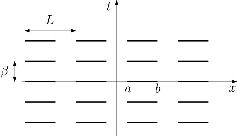 Figure 1
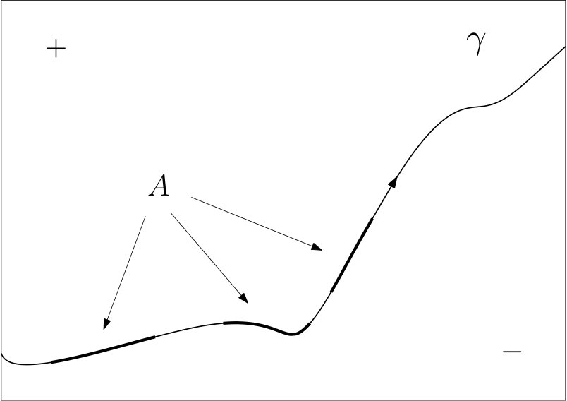 Figure 2
 Figure 3
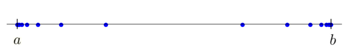 Figure 3
Peer Reviews
No public reviews on file for this paper yet. If you reviewed it on a platform where reviews are public (OpenReview, ICLR, NeurIPS, ICML), you can paste yours below so the community can read it here.
Videos
No videos yet. Explain this paper in a talk, walkthrough, or lecture? Add one.
Modular Hamiltonian of a chiral fermion on the torus
David Blanco
Departamento de Física, FCEN, Universidad de Buenos Aires and IFIBA-CONICET
1428 Buenos Aires, Argentina
Guillem Pérez-Nadal
Departamento de Física, FCEN, Universidad de Buenos Aires and IFIBA-CONICET
1428 Buenos Aires, Argentina
Abstract
We consider a chiral fermion at non-zero temperature on a circle (i.e., on a torus in the Euclidean formalism) and compute the modular Hamiltonian corresponding to a subregion of the circle. We do this by a very simple procedure based on the method of images, which is presumably generalizable to other situations. Our result is non-local even for a single interval, and even for Neveu-Schwarz boundary conditions. To the best of our knowledge, there are no previous examples of a modular Hamiltonian with this behavior.
I Introduction
In recent years, the study of entanglement and its measures has proven to be very useful in unveiling some of the deepest properties of Quantum Field Theory (QFT). Entanglement measures are based on the reduced density matrix, or equivalently on (minus) its logarithm, the modular Hamiltonian. Among other applications, the knowledge of modular Hamiltonians was essential for the proof of the averaged null energy condition Faulkner:2016mzt , the derivation of quantum energy inequalities Blanco:2013lea ; Blanco:2017akw and the formulation of a well-defined version of the Bekenstein bound Casini:2008cr . Modular Hamiltonians also played a key role in applications to holography, the most notable case probably being the derivation of the linearized Einstein equations in the bulk from entanglement properties of the boundary Conformal Field Theory (CFT) Faulkner:2013ica ; Lashkari:2013koa ; Blanco:2018riw ; Swingle:2014uza .
There are only few cases where modular Hamiltonians have been computed. The result is universal and local for the vacuum of any QFT reduced to Rindler space Unruh:1976db ; Bisognano:1976za , and from this result one can also derive CFT expressions for the vacuum reduced to a ball in the plane Casini:2011kv , for a thermal state reduced to an interval in the plane in 1+1 dimensions Hartman:2015apr and for the vacuum reduced to an interval in the cylinder in 1+1 dimensions Cardy:2016fqc . In these cases the modular Hamiltonian turns out to be local, but non-local contributions are expected to appear in general. This was first shown explicitly with the calculation of the modular Hamiltonian of the vacuum state reduced to an arbitrary set of disjoint intervals in 1+1 dimensions for free chiral fermions on the plane Casini:2009vk , later for the cylinder Klich:2015ina and more recently for free chiral scalars on the plane Arias:2018tmw . Another notable result is the modular Hamiltonian for the vacuum state of any QFT reduced to regions ending on a null plane Casini:2017roe .
In this paper we compute a new modular Hamiltonian, namely that corresponding to a chiral fermion on the circle at non-zero temperature (i.e., on the torus in Euclidean language). Our analysis is based on the method of images applied to the calculation of the Euclidean propagator, which enables us to map the problem to a similar problem on the plane. The method turns out to be very simple, and we expect it to have applications beyond the case of chiral fermions. Our result is non-local even for a single interval, even for Neveu-Schwarz (antiperiodic) boundary conditions.
II Modular Hamiltonian from the resolvent
Consider a chiral fermion on a circle of length . The Hamiltonian is
[TABLE]
where the sign depends on the chirality. Suppose that the field is in a thermal state with inverse temperature . The purpose of this paper is to compute the reduced density matrix corresponding to a subset of the circle or, equivalently, the modular Hamiltonian
[TABLE]
Since the global state is Gaussian, the reduced density matrix is also Gaussian and hence the modular Hamiltonian has the form
[TABLE]
As shown in peschel2003calculation , the kernel is related to the two-point function () by
[TABLE]
where both and are viewed as operators acting on functions on . This equation can be rewritten as
[TABLE]
where is the resolvent of ,
[TABLE]
as can be easily checked by explicitly performing the integral in (5). Thus, the problem of computing the modular Hamiltonian reduces to that of finding the resolvent of .
III The method of images
Our strategy for computing the resolvent is based on the method of images applied to the calculation of the Euclidean propagator , which is defined by
[TABLE]
for and by analytic continuation for other values of and , where is the step function. Depending on the spin structure chosen on the circle, the Euclidean propagator can be either periodic or antiperiodic in with period , and it is antiperiodic in with period . Due to these quasiperiodicity properties, we may view as a section of a line bundle over a torus of circumferences and . Inserting (1) in (III) one sees that the Euclidean propagator satisfies
[TABLE]
for . Identifying with via the map , this equation says precisely that is analytic in for and has a simple pole at with residue . In other words,
[TABLE]
where is analytic in for . In the language of complex variables the quasiperiodicity conditions read
[TABLE]
where , , and . Eqs. (9) and (10) have a unique solution. Indeed, the difference between two solutions is analytic for and satisfies (10), so it is analytic and bounded throughout the complex plane. By Liouville’s theorem, such a function is necessarily a constant, so the antiperiodicity in the imaginary direction implies . In order to find the solution, let us first look at the limiting case , where the torus becomes a plane and the quasiperiodicity conditions (10) are replaced by the condition that vanish at infinity. Since the only analytic function that vanishes at infinity is the zero function, the solution of Eq. (9) on the plane is
[TABLE]
Going back to the torus, i.e., to generic values of and , we can solve Eqs. (9) and (10) by the method of images,
[TABLE]
where is the lattice
[TABLE]
and . Indeed, the function (12) clearly has the form (9), and one can easily check that it satisfies the quasiperiodicity conditions (10).
Let now . It is clear from (III) that (note that it is important to take the limit from above, because if we take it from below we pick a delta function). With our identification of with , we thus have
[TABLE]
so, by (12),
[TABLE]
where , see Fig. 1,
and
[TABLE]
for . The main reason why the method of images is useful for us is that Eq. (15) also holds for the powers of the operators involved,
[TABLE]
for any , where denotes the kernel of the operator (not to be confused with ). We can see this by induction. First, the above equation is satisfied for (this is Eq. (15)). And second, if it holds for some we have
[TABLE]
In the third equality we have used the translational invariance of , and in the fourth we have defined and . Eq. (17) implies that the method of images works for any function of which can be expressed as a power series. In particular, it works for the resolvent,
[TABLE]
In the case of zero temperature, , the terms with do not contribute to the sum (12), so the lattice effectively reduces to and, in consequence, the region reduces to an arrangement of segments in the real line. The resolvent is well-known in that case Casini:2009vk , so we can use it to obtain via the above equation. To the best of our knowledge, is not known for generic temperatures, where is a collection of segments distributed all over the complex plane, but it can be easily computed as we will explain in the next section.
IV The resolvent for a generic set of segments in the plane
Consider a curve in the complex plane with both endpoints at infinity, and a subset , see Fig. 2. As shown in the figure, divides the plane into two regions: the one to the left of the curve ( region) and the one to the right ( region); if is the real line these regions are the upper and lower half-planes respectively.
The purpose of this section is to compute the resolvent of the operator with kernel
[TABLE]
for , where denotes the limit of as is approached from the region. This resolvent is known in the case where is the real line Casini:2009vk ; as we will see, the computation for generic is remarkably simple.
We will first obtain an expression for the powers of . Then we will insert that expression into the expansion of the resolvent in powers of and find that it is easy to perform the sum. For the square we have
[TABLE]
where
[TABLE]
Note that
[TABLE]
Indeed, if is a slight deformation of which has the same endpoints but travels through the region we have
[TABLE]
where the contour in the last integral encircles , and hence . We can rewrite (IV) as an operator equation,
[TABLE]
Now, using (23) and (25) it is a simple matter to check that the operator-valued function
[TABLE]
satisfies . In turn, this implies for the -th derivative , as can be easily shown by induction. Noting that , we thus obtain
[TABLE]
Inserting this expression into the expansion of the resolvent in powers of (which is a geometric series) we recognize the Taylor series of ,
[TABLE]
where in the last step we have used (23) and defined
[TABLE]
Eq. (IV) gives the resolvent for a generic subset of a generic curve. Let us particularize it to the case where is a collection of horizontal segments, with . In this case the integral (22) is easily computed,
[TABLE]
and, using the relation (there is a principal part implicit in the first term), the resolvent (IV) takes the form
[TABLE]
This result agrees with that of Casini:2009vk in the case where is contained in the real line.
V Modular Hamiltonian on the torus
Our last step is to use the resolvent just computed to obtain the resolvent on the torus by the method of images, Eq. (19), and from it the modular Hamiltonian. For simplicity, we concentrate on the case where is a single interval, , but the analysis that follows extends straightforwardly to the general case of multiple intervals. Setting in (30) yields
[TABLE]
This series is ambiguous because it is not absolutely convergent. However, its second derivative is unambiguous,
[TABLE]
where is the Weierstrass elliptic function (see sigma for a review). Since the latter is related to the Weierstrass sigma function
[TABLE]
by , we conclude that
[TABLE]
where
[TABLE]
and are undetermined constants. The Weierstrass sigma function is quasiperiodic,
[TABLE]
where and . Therefore, is also quasiperiodic,
[TABLE]
where . Substituting the resolvent (IV) with into (19), and using (35), (36) and (38), we obtain for the resolvent on the torus
[TABLE]
where
[TABLE]
which does not need the regulator because the argument of the logarithm is real and positive, and
[TABLE]
Note that the constant has dropped out because only involves the difference , see (IV). Note also that the summand above may diverge exponentially as grows; preventing this divergence fixes . Therefore, the ambiguity in disappears from the resolvent on the torus. Now, has the following properties: (i) it is analytic in for except for a simple pole at with residue ; and (ii) it is quasiperiodic,
[TABLE]
By the argument we gave under Eq. (10), there is only one function with these properties. This function is
[TABLE]
where
[TABLE]
(recall that ). Indeed, is analytic, has a simple zero at the origin with and does not vanish anywhere else in the region . Together with quasiperiodicity, this implies that the second ratio in (43) is analytic, from which property (i) follows. On the other hand, Eq. (37) and the relation imply
[TABLE]
from which property (ii) follows. Thus, Eqs. (V) and (43) give the resolvent on the torus. Inserting it into (5), noting that the terms with a delta function cancel and changing the variable of integration from to yields the modular Hamiltonian,
[TABLE]
We have checked that this result coincides with known results in the limits Hartman:2015apr and Klich:2015ina , including the presence of a non-local term in the case (periodic, or Ramond, boundary conditions). In order to obtain a more explicit expression for and generic, note from (45) that is quasiperiodic in ,
[TABLE]
where ( is odd and satisfies , so is real). Therefore,
[TABLE]
where
[TABLE]
Now, for fixed, the argument of the delta function above decreases monotonically from to as goes from to , and hence it has a unique zero for each . For this is . Noting that one easily obtains the local contribution to the modular Hamiltonian,
[TABLE]
where
[TABLE]
In order to obtain the non-local contribution (i.e., the contribution from the remaining values of ), note that the delta function in (V) selects precisely those pairs of points for which is periodic. On the other hand, satisfies a second quasiperiodicity property, analogous to (47) with replaced by and replaced by . Using these two facts, one can rewrite the integral on the right-hand side of (48) in terms of a contour integral encircling a single pole. Evaluating the latter by residues finally yields the non-local contribution to the modular Hamiltonian,
[TABLE]
For fixed, this non-local term has support in an infinite number of points which tend to accumulate near the endpoints of the interval, as shown in Fig. 3. Thus, the modular Hamiltonian is highly non-local, both for Ramond ( and Neveu-Schwarz () boundary conditions.
The above is a novel explicit example of a modular Hamiltonian, which has the interesting property of being highly non-local even for a single interval, for any choice of boundary conditions. It thus opens a new window for the exploration of the entanglement properties of QFT. While this manuscript was nearing completion a work with related results appeared Hollands:2019hje , and another similar study Fries:2019ozf appeared after this paper was first announced on arXiv. We leave the comparison between the three analyses for future work.
Acknowledgements.— The authors would like to thank Horacio Casini, Pascal Fries, Alan Garbarz, Gaston Giribet, Andrés Goya, Martín Mereb and Ignacio Reyes for very fruitful discussions. This work was supported by CONICET and Universidad de Buenos Aires, Argentina.
The reference list from the paper itself. Each links out to its DOI / PubMed record.
- 1(1) T. Faulkner, R. G. Leigh, O. Parrikar, and H. Wang, “Modular Hamiltonians for Deformed Half-Spaces and the Averaged Null Energy Condition,” JHEP , vol. 09, p. 038, 2016.
- 2(2) D. D. Blanco and H. Casini, “Localization of Negative Energy and the Bekenstein Bound,” Phys. Rev. Lett. , vol. 111, no. 22, p. 221601, 2013.
- 3(3) D. Blanco, H. Casini, M. Leston, and F. Rosso, “Modular energy inequalities from relative entropy,” JHEP , vol. 01, p. 154, 2018.
- 4(4) H. Casini, “Relative entropy and the Bekenstein bound,” Class. Quant. Grav. , vol. 25, p. 205021, 2008.
- 5(5) T. Faulkner, M. Guica, T. Hartman, R. C. Myers, and M. Van Raamsdonk, “Gravitation from Entanglement in Holographic CF Ts,” JHEP , vol. 03, p. 051, 2014.
- 6(6) N. Lashkari, M. B. Mc Dermott, and M. Van Raamsdonk, “Gravitational dynamics from entanglement ’thermodynamics’,” JHEP , vol. 04, p. 195, 2014.
- 7(7) D. Blanco, M. Leston, and G. Pérez-Nadal, “Gravity from entanglement for boundary subregions,” JHEP , vol. 18, p. 130, 2018.
- 8(8) B. Swingle and M. Van Raamsdonk, “Universality of Gravity from Entanglement,” ar Xiv e-print , 2014.