Assessing non-linear models for galaxy clustering III: Theoretical accuracy for Stage IV surveys
Benjamin Bose, Kazuya Koyama, Hans A. Winther

TL;DR
This study compares two models for galaxy clustering in large surveys, finding the TNS model more accurate and robust across various tests, which is crucial for precise cosmological measurements.
Contribution
The paper provides a comprehensive MCMC comparison of TNS and EFTofLSS models, establishing the TNS model's superior validity range for Stage IV survey analyses.
Findings
TNS model's validity range is broader and more robust.
EFTofLSS model struggles with highly biased tracers and large volumes.
Constraints on the growth rate are stronger with the TNS model.
Abstract
We provide in depth MCMC comparisons of two different models for the halo redshift space power spectrum, namely a variant of the commonly applied Taruya-Nishimichi-Saito (TNS) model and an effective field theory of large scale structure (EFTofLSS) inspired model. Using many simulation realisations and Stage IV survey-like specifications for the covariance matrix, we check each model's range of validity by testing for bias in the recovery of the fiducial growth rate of structure formation. The robustness of the determined range of validity is then tested by performing additional MCMC analyses using higher order multipoles, a larger survey volume and a more highly biased tracer catalogue. We find that under all tests, the TNS model's range of validity remains robust and is found to be much higher than previous estimates. The EFTofLSS model fails to capture the spectra for highly biased…
Click any figure to enlarge with its caption.
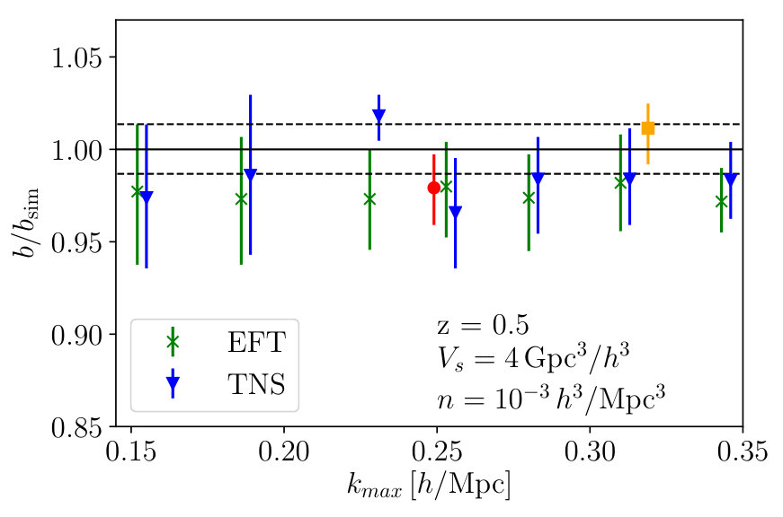 Figure 1
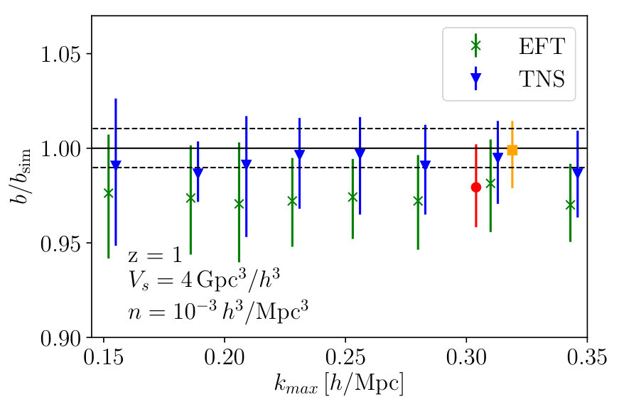 Figure 2
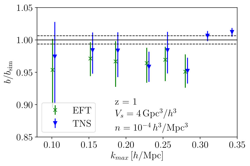 Figure 3
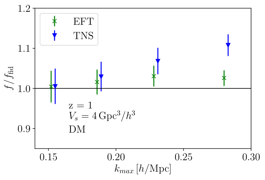 Figure 4
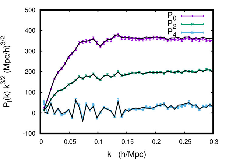 Figure 5
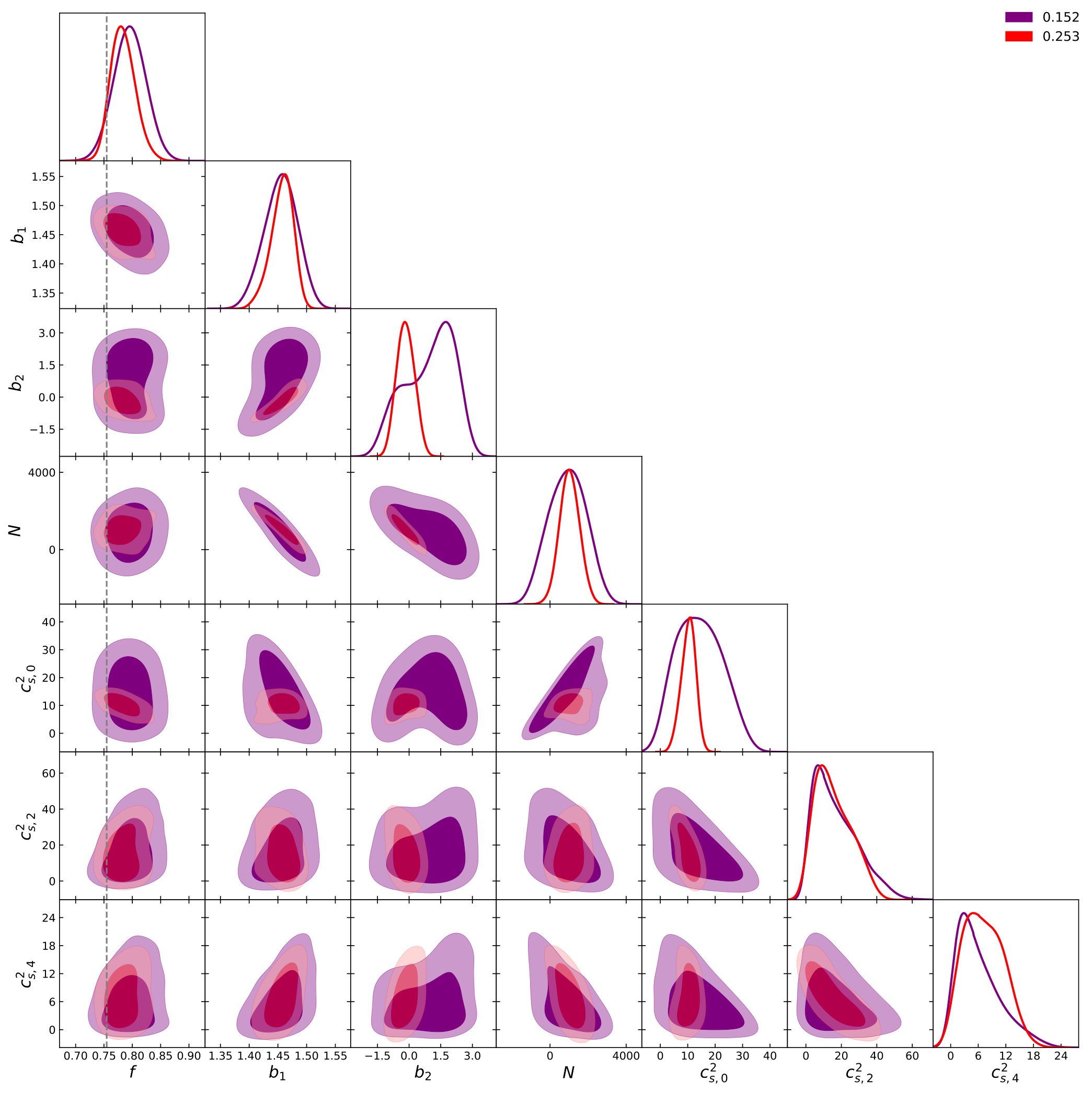 Figure 6
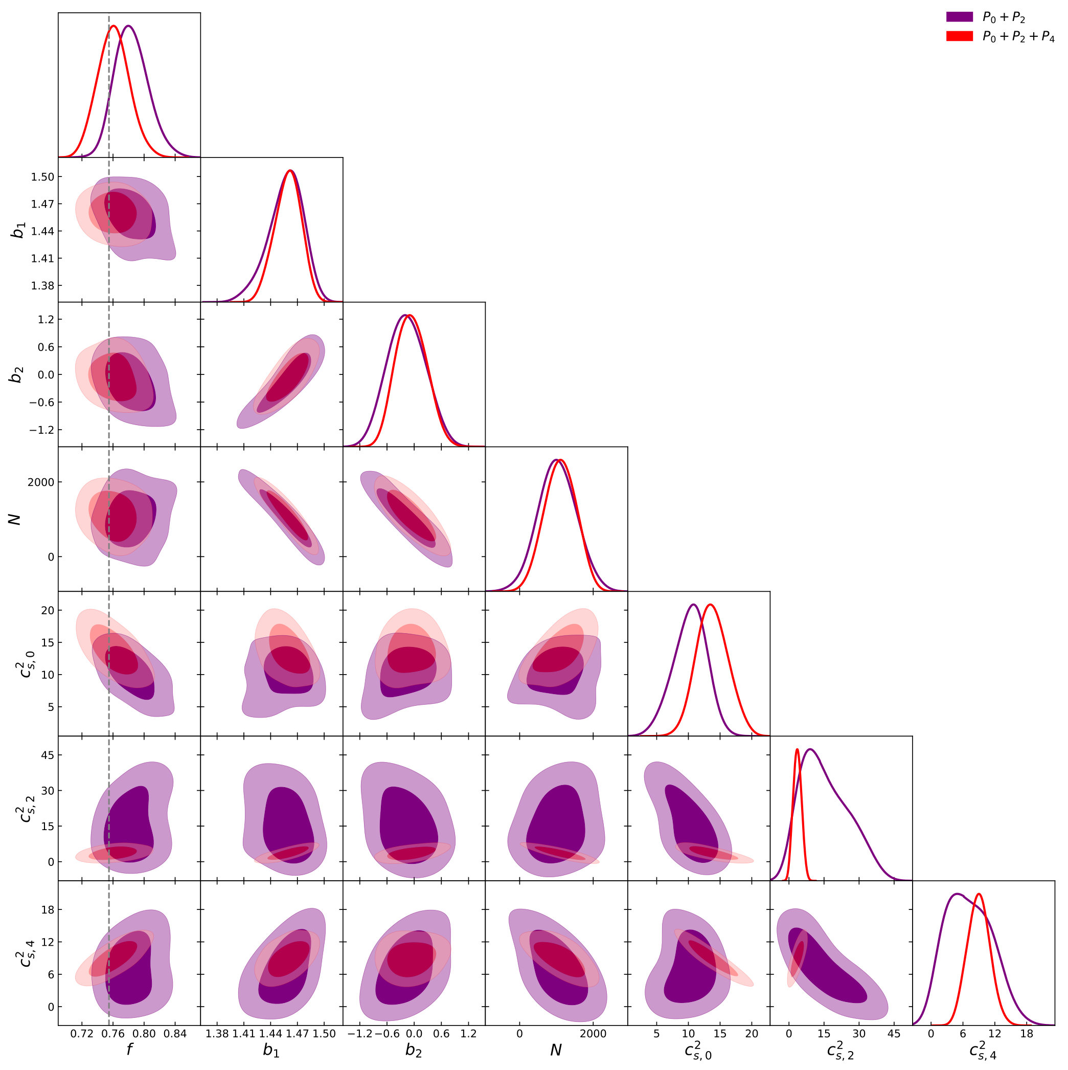 Figure 7
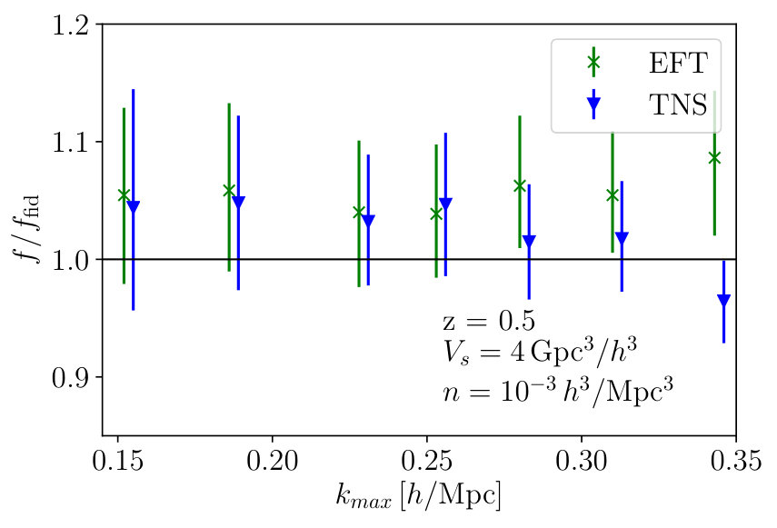 Figure 8
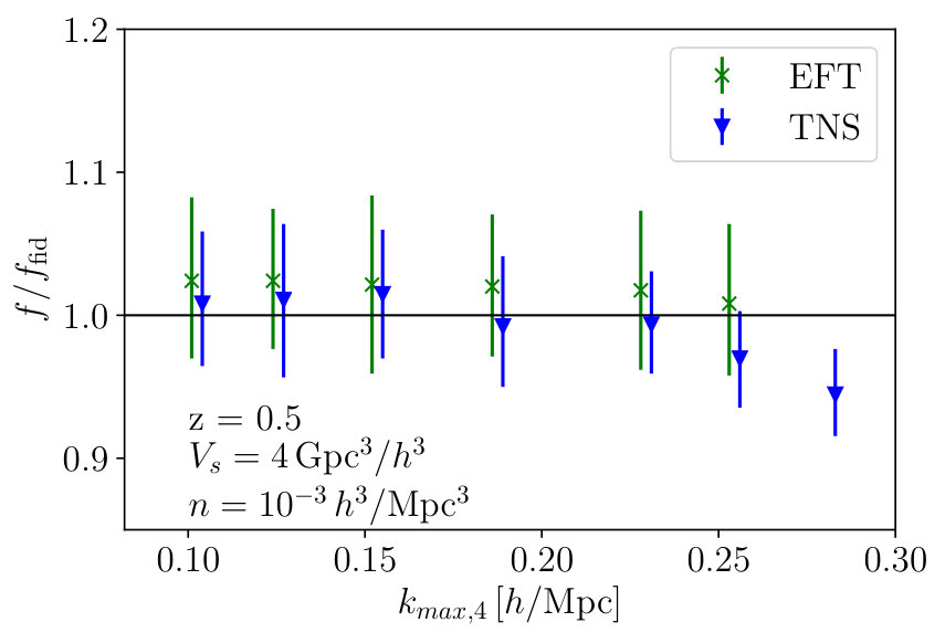 Figure 9
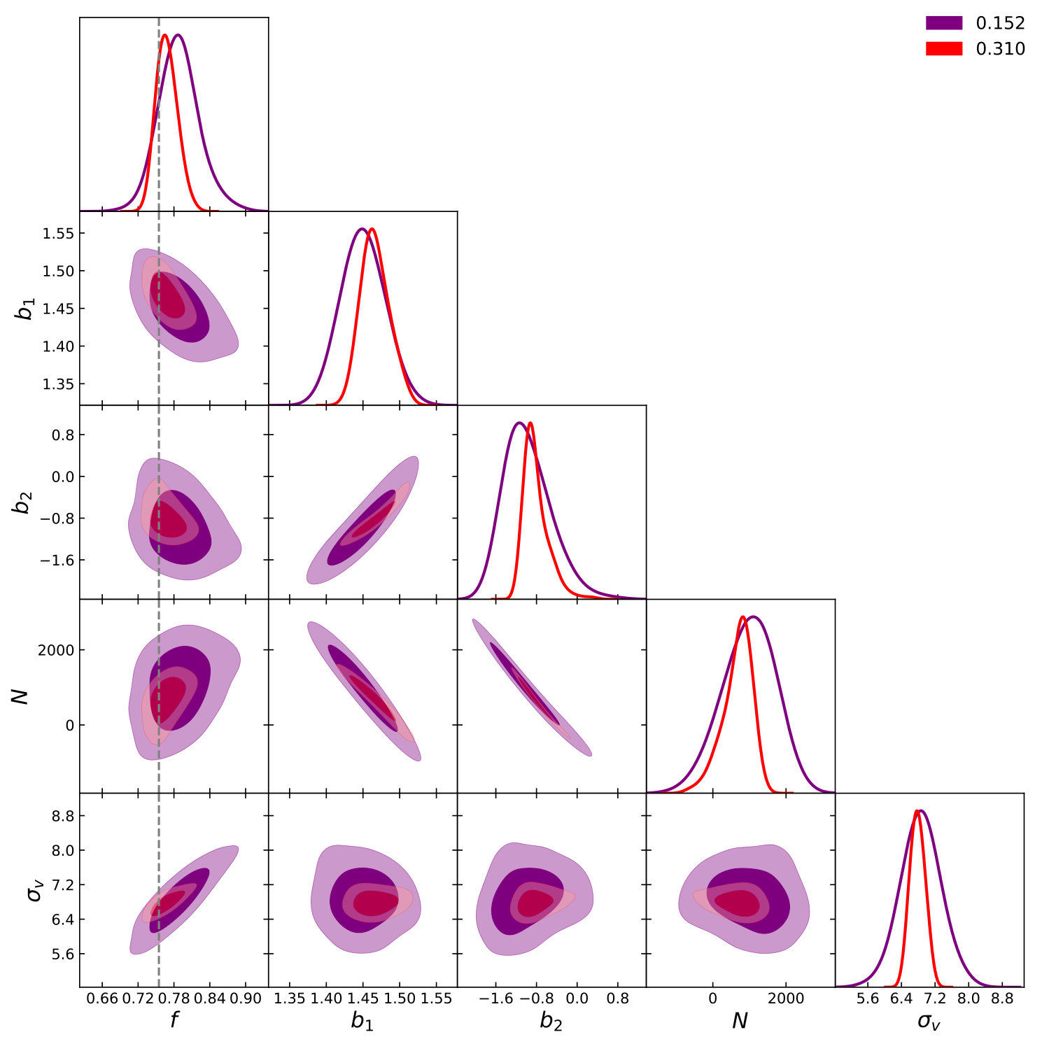 Figure 10
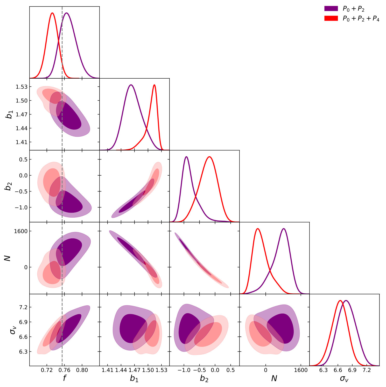 Figure 11
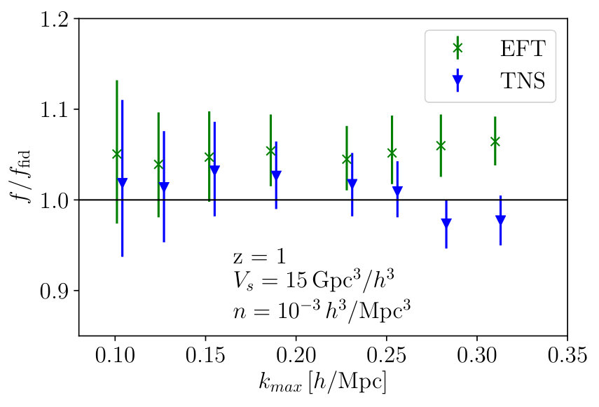 Figure 12
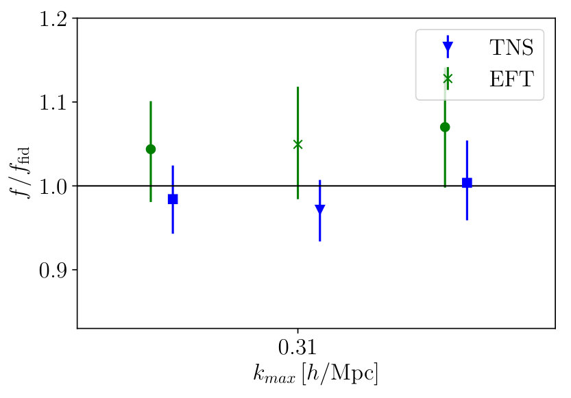 Figure 13
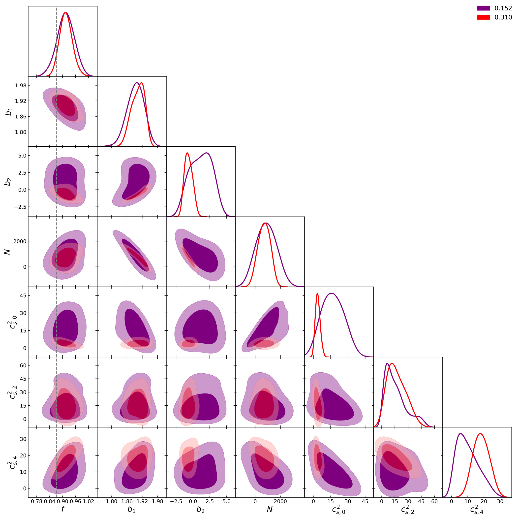 Figure 14
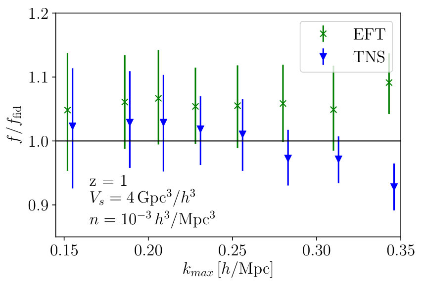 Figure 15
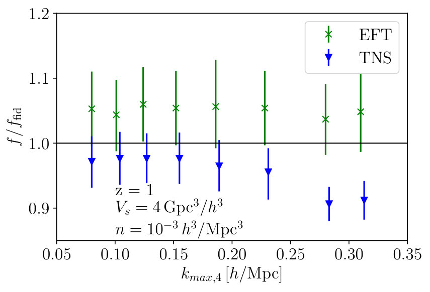 Figure 16
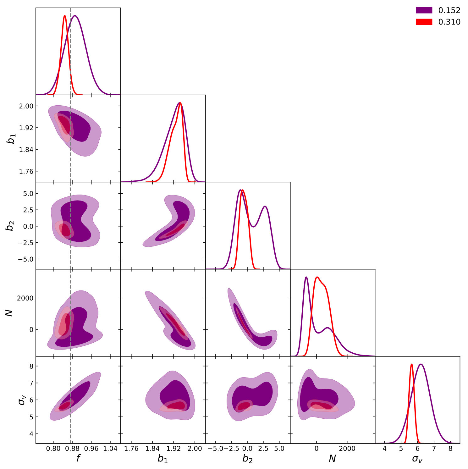 Figure 17
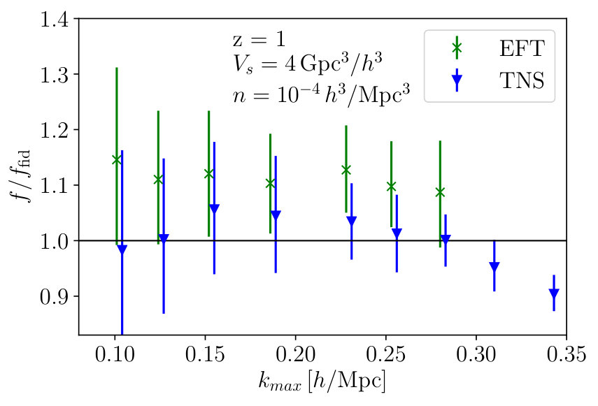 Figure 18
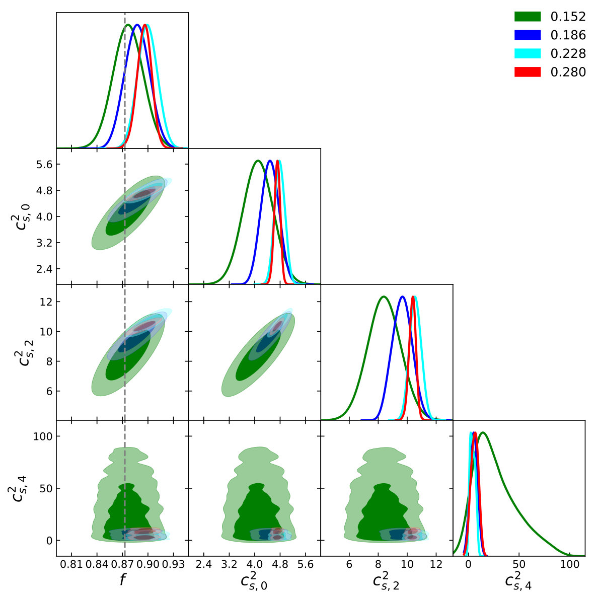 Figure 19
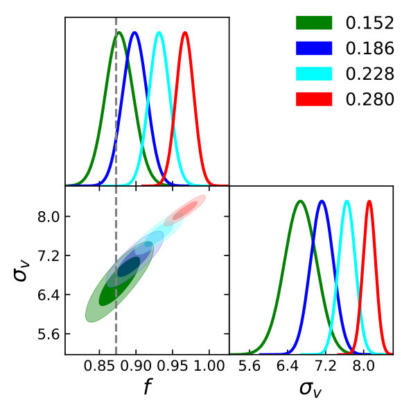 Figure 20
| Multipoles | TNS-based model | EFTofLSS-based model | |||
|---|---|---|---|---|---|
| 1 | 4 | ||||
| 1 | 4 | ||||
| 0.5 | 4 | (0.253) | |||
| 0.5 | 4 | ||||
| 1 | 15 | ||||
| 1 | 4 |
Peer Reviews
No public reviews on file for this paper yet. If you reviewed it on a platform where reviews are public (OpenReview, ICLR, NeurIPS, ICML), you can paste yours below so the community can read it here.
Videos
No videos yet. Explain this paper in a talk, walkthrough, or lecture? Add one.
Assessing non-linear models for galaxy clustering III: theoretical accuracy for Stage IV surveys
Benjamin Bose
Departement de Physique Theorique, Universite de Geneve, 24 quai Ernest Ansermet, 1211 Geneve 4, Switzerland
Kazuya Koyama
Institute of Cosmology & Gravitation, University of Portsmouth, Portsmouth, Hampshire, PO1 3FX, UK
Hans A. Winther
Institute of Cosmology & Gravitation, University of Portsmouth, Portsmouth, Hampshire, PO1 3FX, UK
Institute of Theoretical Astrophysics, University of Oslo, 0315 Oslo, Norway
Abstract
We provide in depth MCMC comparisons of two different models for the halo redshift space power spectrum, namely a variant of the commonly applied Taruya-Nishimichi-Saito (TNS) model and an effective field theory of large scale structure (EFTofLSS) inspired model. Using many simulation realisations and Stage IV survey-like specifications for the covariance matrix, we check each model’s range of validity by testing for bias in the recovery of the fiducial growth rate of structure formation. The robustness of the determined range of validity is then tested by performing additional MCMC analyses using higher order multipoles, a larger survey volume and a more highly biased tracer catalogue. We find that under all tests, the TNS model’s range of validity remains robust and is found to be much higher than previous estimates. The EFTofLSS model fails to capture the spectra for highly biased tracers as well as becoming biased at lower wavenumbers when considering a very large survey volume. Further, we find that the marginalised constraints on for all analyses are stronger when using the TNS model.
I Introduction
Future spectroscopic galaxy surveys will have the power to probe the growth rate of cosmological structure, , to an unprecedented level of precision. The measurement of the anisotropy in the galaxy distribution, the so called redshift space distortions (RSD) Hamilton (1997), is one such way to get a measure of this, and will tell us a lot about gravity and cosmology. This comes with the caveat that we apply an accurate theoretical model to the data. If the model we apply is not sufficiently accurate then the value of we infer from the data will not be the ’true’ value, and our picture of nature will be biased.
This caveat becomes very important in the context of stage IV surveys such as Euclid111www.euclid-ec.org Laureijs et al. (2011) and the Dark Energy Spectroscopic Instrument (DESI)222www.desi.lbl.gov Aghamousa et al. (2016). The issue here is that the data will come with very small observational errors which will greatly penalize small inaccuracies in our modelling. This then requires that applied models be heavily scrutinized and tested before being applied to real observational data and drawing conclusions about the universe.
The two point correlation function, or power spectrum, has been the observable commonly used in past data sets Blake et al. (2011); Reid et al. (2012); Macaulay et al. (2013); Beutler et al. (2014); Gil-Marín et al. (2016); Simpson et al. (2016); Beutler et al. (2017). As it uses only galaxy pairs, it can be measured with relatively high statistical significance, a significance that is enhanced as we move to smaller galaxy separations. For this reason, modeling the smaller scales becomes an attractive means of tightening constraints on growth. But as mentioned, this needs to be done carefully and any potential power spectrum models must be well validated. These models usually come with additional degrees of freedom (dof) that are necessary to model largely unknown physics, such as non-linear matter dynamics or the bias between galaxy and dark matter distributions. These so called nuisance parameters degrade constraints on cosmology and gravity in data analyses as they are marginalised over. Thus, a model whose nuisance parameters are few and non-degenerate with cosmological ones is strongly preferred.
In a previous work Bose et al. (2019), we identified two prominent and competing semi-perturbative models for the redshift space galaxy power spectrum. Namely, the TNS model Taruya et al. (2010) with a Lorentzian damping prefactor and an effective field theory of LSS (EFTofLSS) Baumann et al. (2012); Carrasco et al. (2012) inspired model. Both these models attempt to model the quasi non-linear regime of structure formation in different ways and both were shown to do well in reproducing the measured halo power spectrum from COLA Tassev et al. (2013); Izard et al. (2016); Howlett et al. (2015); Valogiannis and Bean (2017); Winther et al. (2017) simulations when was fixed to its fiducial value. In that work we were concerned with determining the degeneracies of each model’s dofs as well as forecasting the model’s constraint on in the context of a future spectroscopic survey. We also obtained realistic constraints in a limited Markov Chain Monte Carlo (MCMC) analysis.
In this work we go a step further in testing how robust each of these model’s accuracy is by making use of various data sets in the setting of a real data analysis. In particular, we use a large suite of high resolution COLA simulations to test the accuracy of the TNS and EFTofLSS model. We do this by letting the growth rate of structure and all additional model dof to vary in further MCMC analyses. We then identify where each model fails to reproduce the fiducial growth rate and compare their respective constraints.
This paper is organized as follows: In Sec. II we present the biased tracer RSD models. In Sec. III we present the simulations we use and our primary MCMC analysis. In Sec. IV we present the results from additional analyses testing the robustness of the models to different data sets and errors. In Sec. V we summarize our findings and conclude.
II Theoretical Models
We will begin by presenting the two biased tracer RSD models. These were described and studied in Bose et al. (2019) and we refer the reader to this paper for more explicit information on the exact formulas.
The first is the TNS RSD model Taruya et al. (2010) combined with the tracer bias model of McDonald and Roy McDonald and Roy (2009). The model is given by
[TABLE]
where the superscript S denotes the power spectrum in redshift space, is the cosine of the angle between and the line of sight and are the 1-loop galaxy power spectra with the bias model of McDonald and Roy (2009) implicitly included. The logarithmic growth rate of structure is also implicit (again see Bose et al. (2019)). The real space power spectra are all constructed within standard Eulerian perturbation theory at the 1-loop level 333 Note that within the loop integrals we parametrise the integrated wave number as and then take a UV cut-off of . We have found that the integrals are insensitive to this choice at or above the chosen value. See Makino et al. (1992) for a discussion on this issue. , , and are perturbative RSD correction terms Taruya et al. (2010), while the prefactor, , is phenomenological and here takes a Lorentzian form
[TABLE]
where is a free parameter and represents the velocity dispersion of the tracers. We again refer the reader to Bose et al. (2019) for the formulas for the perturbative components of the model, along with the explicit dependency on the independent free bias parameters , where is the linear bias, is the second order bias term and is a stochasticity term.
We remark that this model is very similar to the model chosen for the BOSS analysis Beutler et al. (2017) and has been very well studied and successful in reproducing simulation measurements. It has also shown robustness when considering alternative theories of gravity (see for example Bose and Koyama (2016); Bose et al. (2018a)). The full set of nuisance parameters in this model is .
The second model we consider is one based on the EFTofLSS prescription for the redshift space dark matter spectrum (see de la Bella et al. (2017) for example). To this we introduce the tracer bias model of McDonald and Roy (2009) (same as used in Eq. 1) as well as use a resummation scheme Vlah et al. (2016); de la Bella et al. (2017) 444 See Matsubara (2008); Senatore and Zaldarriaga (2014); Lewandowski et al. (2015) for alternative schemes that have been shown to be equivalent to the one adopted here in Bose et al. (2018b). for the dark matter 1-loop power spectra only as these are the leading contributions to the oscillations associated with baryon acoustic oscillations when fitting the counter terms. Note that we do not do a full resummation of the redshift space spectrum as in de la Bella et al. (2017), but the impact of resummation has also been shown to have a low impact on the best-fit analysis conducted in de la Bella et al. (2018) where they consider halos in redshift space. The expression is given as
[TABLE]
where are the sound speed parameters of EFTofLSS, is the linear growth factor, is the primordial power spectrum 555Produced using CAMB Lewis and Bridle (2002) for example. and
[TABLE]
The nuisance parameters of this model are which is an additional 2 over the TNS approach described by Eq. 1. A slight variant of Eq. 3 was found to be well motivated in de la Bella et al. (2018) through a Bayesian criterion which accounts for number of free parameters of the model as well as fits to simulations. On the other hand, the proper treatment of bias in EFTofLSS has been presented in Perko et al. (2016) but comes with 10 nuisance parameters (compared to the 6 of Eq. 3). Given this, it is very unclear whether this model would be favoured over the ones presented here.
In Eq. 1 and Eq. 3 cosmological parameter dependence enters through the primordial power spectrum with the parameter 666 governs the amplitude of density perturbations at Mpc/ where is the tophat window function. being completely degenerate with the linear growth factor . In our analysis we fix or equivalently . Further we fix a fiducial cosmology and in doing so any results made on the robustness or range of validity are consequently conservative. Any results on constraining power are conversely optimistic as we do not marginalize over cosmology.
III Simulations
The simulations used in this paper were created using a modified version Winther et al. (2017) of the L-PICOLA code Howlett et al. (2015). These simulations use the fast approximate COmoving Lagrangian Acceleration (COLA) method Tassev et al. (2013). We created a set of realisations of a CDM cosmology defined by . The simulations had particles in a box of with grid-cells. We also ran a full N-body simulation using the RAMSES Teyssier (2002) code that had the same initial condition as one of the COLA simulations which allowed us to check the accuracy of our results. These results can be found in Appendix A.
From the simulations we computed halo catalogs using a friends-of-friends (FOF) algorithm777The halo finder MatchMaker has been included in the MGPICOLA code used in this paper. See https://github.com/damonge/MatchMaker and https://github.com/HAWinther/MG-PICOLA-PUBLIC. The halo catalogs were then trimmed based on a number density criterion (we considered samples with and ) giving us the mock data from which we computed the RSD multipoles and the real-space power spectrum.
PICOLA multipoles are measured using the distant-observer approximation. That is, we assume the observer is located at a distance much greater then the box size (), so we treat all the lines of sight as parallel to the chosen Cartesian axes of the simulation box. Next, we use an appropriate velocity component ( or ) to displace the position of a matter particle or dark matter halo to put it into redshift space. We then average over three line-of-sight directions. We further average over the PICOLA realisations. These are calculated at both and .
IV Results
Our aim here is to test the accuracy of each of the models outlined in Sec. II and their ability to model the non-linear regime. To do this we perform a fit to the simulated data. First we perform an angular decomposition of in terms of the multipole moments. This is what is commonly done in real data analyses Beutler et al. (2014, 2017). These multipoles can be defined as
[TABLE]
where denote the Legendre polynomials and is given by Eq. 1 or Eq. 3. For the majority of our analyses we utilize the monopole () and quadrupole (). The inclusion of the hexadecapole is known to significantly restrict the range of validity/applicability of the models considered. This partly comes from the fact that each multipole has a different damping scale and so we do not expect a model with less RSD parameters than the number of multipoles, to be able to capture all of them accurately. Higher order multipoles have finer features as a function of angle and so may also pick out inaccuracies in the full anisotropic spectrum. Since the information gain is roughly proportional to each independent one can access, a restriction in range results in a reduction in valuable cosmological information. So, since the monopole and quadrupole contain most of the RSD information we first perform fits using only and and then introduce but restrict the scales to which we compare it to the data. This is what was done in the BOSS analysis Beutler et al. (2017). An analysis using this procedure is outlined in a later subsection.
Using the multipoles we perform a large number of MCMC analyses on the simulation data in order to test the model’s recovery of the fiducial growth rate at various inclusion of scales. We vary all model nuisance parameters in these analyses as well as , imposing the following flat priors .
We model our log likelihood using the statistic
[TABLE]
where is the covariance matrix between the different multipoles, is the smallest physical scale used in the analysis and conversely is the largest physical scale. We apply linear theory to model the covariance matrix between the multipoles (see Appendix C of Taruya et al. (2010) for details). This has been shown to reproduce N-body results up to at Taruya et al. (2010). Again, for the majority of our analyses we only consider since these have the largest signal and contain most of the RSD information. We do consider the impact of in a later subsection.
We wish to work within the context of stage IV surveys. Therefore, we will concentrate our analysis on which will be a key redshift targetted by the Euclid mission Amendola et al. (2018). Further we use planned tracer number density, and a realistic observational volume888Note that this depends on the bin-width, and here the volume chosen corresponds to a bin width of . of Aghamousa et al. (2016); Majerotto et al. (2012); Amendola et al. (2018) in our covariance matrix in Eq. 6 999Note we also assume a linear bias in the covariance as determined by the simulation halo catalogs, i.e. the ratio of to . For the catalog we take for and at .. This volume and number density are also reflected in our halo catalogues and unless otherwise stated, these will be the default parameters of the analysis.
We will also provide supplementary analyses which will consider the hexadecapole, a lower redshift where non-linear structure formation is greater, a different catalog of halos with a lower number density and the impact of having a larger survey volume which will better reflect the combined power of the whole survey over many bins.
IV.1 Dark Matter
Before considering halos, we look at the dark matter distribution as it will be instructive to understand the capabilities of the pure RSD models, i.e. setting and in Eq. 1 and Eq. 3. Again, this is done at using . Fig. 1 shows the two-dimensional posterior distributions for the TNS and EFTofLSS models when we only consider dark matter for various used in Eq. 6 while Fig. 2 shows the marginalised constraints on as a function of . We clearly see both models become biased with a criterion in their recovery of the fiducial value of at around . The TNS model diverges quickly as we include even smaller scales in the analysis while the EFTofLSS model remains biased but this bias does not seem to increase significantly with the inclusion of smaller scales. This is likely due to the fact that TNS has one free parameter to describe the damping thus it cannot capture the different damping of and . At the fractional marginalised error on is found to be and for TNS and EFTofLSS respectively.
Secondly, we immediately note from Fig. 1 that there are significant degeneracies between and the model nuisance parameters. This is not a new result for the TNS model Zheng et al. (2017); Bose et al. (2017). What we find here though is that this degeneracy doesn’t weaken as we go to smaller scales. For the EFTofLSS we can see degeneracy between the sound speed parameters and as well. This degeneracy seems to weaken as we push to non-linear scales, especially between , and . The degeneracy between and is also very clear101010Note that only comes with powers of greater or equal to 4 and so in the monopole and quadrupole it does not significantly contribute..
These results can almost be directly compared to those from de la Bella et al. (2017) who also use simulations using the Multidark cosmology in their comparisons. They consider and find that and match the simulation measurements within and respectively up to . These results are significantly higher than what we find here, when we consider bias of cosmological parameters as our criterion for . Our is more comparable to Lewandowski et al. (2015) who determine a reliable scale of at , using a percent level deviation criterion.
IV.2 Halos
Here we investigate the halo multipoles. Fig. 3 shows the marginalised constraints on from the MCMC analyses as a function of for both TNS and EFTofLSS models. We see that again, under a criterion, the models seem to do equally well, and become biased at around , which is significantly larger than the dark matter case. This suggests the bias model provides much added freedom to the models. Further, for TNS, the velocity dispersion of halos is found to be significantly less indicating that different damping of the monopole and quadrupole is not as necessary as in the dark matter case. At the fractional marginalised error on is found to be and for TNS and EFTofLSS respectively.
In Fig. 4 and Fig. 5 we plot the two-dimensional posterior distributions for TNS and EFTofLSS respectively at two different ; and . In the TNS model the degeneracy of with persists but is significantly reduced by the inclusion of non-linear information. Further, degeneracies of with the bias parameters is also reduced with the inclusion of smaller scales. This results in a significant improvement of constraints, with the fractional marginalised error on going from to . In the EFTofLSS case we find a marginal improvement on the fractional error on from to . This is unsurprising due to the larger number of nuisance parameters we need to marginalise over.
IV.3 Analysis at
Here we consider the same survey volume and number density as in the previous subsection but repeat the analysis for . Fig. 6 again shows the mean value of obtained from MCMC analyses using and as a function of . Here we see that again the TNS model does very well in capturing the non-linear RSD halo multipoles without biasing estimates of . On the other hand, the EFTofLSS model becomes slightly biased at . Using the same criterion, we have for the TNS and for the EFTofLSS models. At these we find the fractional marginalised error on to be and for TNS and EFTofLSS respectively. We find at the TNS gives a error which is in fact worse than EFTofLSS despite the smaller parameter space. This is consistent with what we find in Bose et al. (2019), but in that work we did not provide a robust check for the ’true’ .
We again plot the two-dimensional posterior distributions in Fig. 7 and Fig. 8 for TNS and EFTofLSS respectively at two different ; and for TNS and and for EFTofLSS. We find that the parameter degeneracies do not change significantly between and for both models. We also find that at we get similar gains in the constraints on by going to smaller scales. This improves its fractional marginalised error on from to while the EFTofLSS gains less due to its lower , going from to .
So far the TNS model seems to outperform the EFTofLSS model considered here, but this may be because we are not fully utilising all the EFTofLSS free parameters. To better test the capabilities of this model we will next include in our analyses.
IV.4 Impact of hexadecapole
In this subsection we include in the analysis. As mentioned previously, this would severely restrict the range of scales allowed in the analysis since in general modelling of has been found to be poor for the TNS model Beutler et al. (2017); Markovic et al. (2019), and taking it to too high a can result in a biased estimate for . We thus proceed by fixing for and as determined in the previous section (see Fig. 3 and Fig. 6). Then, we include up to a new testing for bias of at the level as before. Note that above we only include terms with in the likelihood given in Eq. 6. We do this for both and .
Fig. 9 and Fig. 10 shows the marginalised constraints as a function of at and respectively. At we see that the TNS becomes slowly biased, with a determined while the EFTofLSS remains unbiased up to . A similar trend is seen at , with the EFTofLSS remaining unbiased all the way up to while the TNS becomes biased before reaches , which at the level is determined to be . This is to be expected as the EFTofLSS allows for individual non-linear damping over the 3 multipoles using all 3 while the TNS only utilises a single free parameter for all 3 multipoles.
We find that at the determined , the marginalised fractional errors on for the TNS model to be and while the EFTofLSS model’s are and at and respectively, where in brackets we indicate the fractional errors determined only using and . This indicates that at , given the hexadecapole’s weak signal and our errors, it doesn’t offer significant additional information on the growth of structure. At it becomes more important and improves constraints significantly for the TNS model whereas for the EFTofLSS it again doesn’t add to the constraints. To gain insight into this we look at the two-dimensional posterior distributions. This is shown in Fig. 11 and Fig. 12 for the TNS and EFTofLSS respectively. In the TNS case, both affects the degeneracy and the constraints on , which has a strong degeneracy with . This results in the noticeable improvement of the marginalised constraints on . In the EFTofLSS case, although improves the constraints on the value of and , these lack a strong degeneracy with (unlike ) and so constraints on are not improved. Further, by including we move the best fit sound speed parameters, , to larger values which reduces the impact of the positivity priors we impose on these parameters. This can explain why at including does not improve the constraint on in the EFTofLSS case.
We also comment on the effect of at in the TNS case. Given the small , we don’t expect to make a noticeable impact. By inspection of the two-dimensional posteriors between the and the analyses (not shown in the paper), we find the parameter degeneracies are not impacted by and it only serves to sharpen most of the marginalised distributions, with the exception of which broadens slightly. Since the constraint on does not degrade significantly we do not investigate this matter further.
Of course all the results so far rely on the errors and scatter of the data. The next three subsections are dedicated to investigating these issues. We first look at the effect of smaller errors.
IV.5 Analysis with
In this section we again concentrate on and the number density but consider a much larger survey volume, which will give a better representation of the errors when using many redshift bins and of the total power of upcoming surveys.
Again, we show the marginalised constraints on from the MCMC analyses as a function of for both TNS and EFTofLSS models in Fig. 13. Immediately we note the EFTofLSS model becomes biased very quickly with a new which is to be expected from Fig. 3 where all the mean values from the MCMC analyses lie significantly above the fiducial. On the other hand the TNS model seems robust against the reduced error bars and barely maintains its original . We find the marginalised fractional errors on at these are and for TNS and EFTofLSS respectively where the bracketed values are from the analysis using . Naturally the TNS constraints are improved significantly maintaining the same , but we also note that the EFTofLSS results also improve despite the far lower . If we maintain the same the EFTofLSS produces a fractional error, but its mean value of is biased by over . Similarly, if we take the TNS model to we find a fractional error of which is comparable to that of the EFTofLSS model.
IV.6 Analysis with
Here we investigate the impact of taking a catalog of more massive halos which translates to a lower number density. On the theoretical side, in the analytic covariance we use and while keeping while the halo catalog measured from simulations makes a number density cut of . This naturally introduces larger errors through the analytic covariance prescription used in Eq. 6 as well as larger scatter in the data due to a lower number of halos. These halos are more massive and so also more biased allowing a test for the flexibility of the bias model, as well as its compatibility with each RSD model.
Once again, Fig. 14 shows the marginalised constraints on from the MCMC analyses as a function of for both models. Similar to Fig. 13, where we considered a larger survey volume, we find the TNS model remains robust achieving . The EFTofLSS model on the other hand becomes biased much earlier at , but this bias seems to be within over a large range of . Again, the fractional errors at the determined are and for the TNS and EFTofLSS model respectively, where the bracketed value is that obtained from the analysis.
To investigate why the EFTofLSS fails at such a small we provide a test in Appendix B where we compare the best fit value of over the full range of to that measured from the simulations. This gives a good indication of what scales the bias model works well at. In particular, we refer the reader to Fig. 19, which supports a failure in the bias model when considering highly biased tracers as seen in Fig. 14 for the EFTofLSS. Further, in Lewandowski et al. (2015); Fujita et al. (2016) which consider the full biased tracer model for EFTofLSS Perko et al. (2016), they consider terms which scale with halo mass. These typically go as or are partially degenerate with the counter terms considered here. Since we observe a biased recovery of in the EFTofLSS-like model we consider at we do not expect these terms to rescue this model. Further, in Appendix B we also find that the Roy and McDonald model seems to break down at the same scales for both TNS and EFTofLSS model and so additional bias terms may be needed in both of these RSD models.
IV.7 Analysis using fewer realisations
Finally, as mentioned in Sec. III, our simulation measurements are the average of realisations and so represent an ideal measurement which are not truly representative of a real observation which will come with scatter which is associated with the errors we’ve attached. Our goal was to test for bias in the models when modelling non-linearity and so we wanted to use highly converged data. In reality, scatter in the data may affect the and in turn introduce a bias if we are to trust a determined from mocks. To investigate this issue we consider 2 sets of 4 realisations taken randomly from the original 35. We repeat the analysis at , using and for twice, once each using the average of both these sets.
Fig. 15 shows the results at for the 2 sets of 4 realisations (shown as circular dots) for the TNS and EFTofLSS models. The plot indicates that the we have determined using the 35 realisations is robust against scatter in the data within the given errors. Further, for both models we find the qualitative shape of the contours does not change appreciably for most of the parameters although central positions and overal sizes do shift within of the realisation average contours for some parameter pairs.
V Discussion and Conclusion
In this work we have extended a number of previous analyses de la Bella et al. (2018); Osato et al. (2018); Markovic et al. (2019) which attempt to discern which models are most apt to model galaxy clustering for upcoming surveys. In particular, we select the two models identified in Bose et al. (2019) as being contenders; the TNS model with a Lorentzian damping factor and an EFTofLSS based model. The EFTofLSS model is similar to one of the leading models identified in de la Bella et al. (2018). We extend previous works by completing many MCMC analyses, using high quality PICOLA simulation data, in which we vary the growth rate of structure as well as all model nuisance parameters (4 for TNS and 6 for EFTofLSS). In particular, we thoroughly test for biased estimation of by the models when considering quasi non-linear scales. These tests are all conducted within the context of upcoming surveys through our selection of the halo catalogs, the simulation volume and our modelling of the RSD-multipole covariance matrix. Further, we test the robustness of the models by considering a different redshift, the hexadecapole, a different halo catalog, a different survey volume and scatter in the data. All our core results are summarised in Table 1.
Overall, we find that the TNS model seems to do better in its constraints on and range of validity than the EFTofLSS model considered here, despite the EFTofLSS’s larger nuisance parameter space. This is not inconsistent with the results of Bose et al. (2019) where a robust test for was not performed. In fact at both redshifts we find a much larger for the models. Although Bose et al. (2019) find that at both models achieve the same , with EFTofLSS giving better marginalised constraints, we find the models push to a higher when properly tested for bias, and the inclusion of these smaller scales may give TNS the edge we see here. But, our conclusion here of course comes with a number of caveats. First, we do not vary the Alcock-Paczynski parameters Alcock and Paczynski (1979) nor consider cosmology beyond , and so do not account for degeneracies between nuisance parameters and these. Second, our EFTofLSS model is phenomenological in the sense that we have treated tracer bias in an ad hoc way by bolting on the bias model of McDonald and Roy (2009). Appendix B suggests that this treatment seems to do well for low biased tracers. The proper treatment of bias within the EFTofLSS follows Perko et al. (2016) and includes 4 more nuisance parameters. With so many nuisance parameters, it seems unlikely that one can achieve better performance in terms of constraints as suggested in de la Bella et al. (2018). But it is still left to be checked if the full biased tracer EFTofLSS model can achieve better constraints than the TNS and we leave that for a future work. Finally, we used an idealised mock data based on dark matter halos and a Gaussian covariance matrix in this work. In order to apply these models to actual observations, we need to take into account the distributions of galaxies within dark matter halos, a survey window function as well as non-Gaussian covariance matrix. These strongly depend on specifications of a specific future survey and we will need to redo the analysis using galaxy mocks designed for the survey.
Beyond constraining power, the models each offer their own advantages and disadvantages. The TNS model is simpler in terms of number of parameters which makes it computationally preferable especially when performing MCMC analyses with a large parameter space where convergence may become an issue. It is flexible in terms of modelling the small scale fingers-of-god damping. Using the Lorentzian damping, it effectively re-sums an expansion of the damping term in . The fact that its constraining power strongly depends on the form of the this damping term indicates that we could improve the model by taking into account the different damping of multipoles. Priors on can also be conceivably achieved through simulations and even observations Hikage et al. (2012), which would improve the model’s constraining abilities. Further, loop corrections in the perturbative part can be added to improve its modelling of the small scales at the considered redshifts. Alternatively, these corrections can be calibrated by simulations Song et al. (2018); Zheng et al. (2018). The model has also been already extended to general theories of gravity and dark energy Bose and Koyama (2016); Bose et al. (2018a).
On the other hand, the EFTofLSS model provides a very systematic way of modelling the small scales and also a way of keeping track of theoretical uncertainties. This will be very important for upcoming surveys where percent level accuracy is needed. It also provides more flexibility in modelling higher order multipoles as seen here, without biasing . Further, priors on the sound speed parameters, can be achieved through multiple redshift measurements and a knowledge of their dependency on redshift Foreman and Senatore (2016). There have also been some attempts to extend this model to modified theories of gravity and dark energy Lewandowski et al. (2017); Cusin et al. (2018); Bose et al. (2018b).
Independent of model comparisons, we find that the TNS with a Lorentzian damping factor as well as the perturbative components modelled within SPT is a very good prescription for galaxy clustering modelling, achieving at and . In previous analyses this particular form of the TNS model was not considered, and rather a Gaussian damping was used with a RegPT Taruya et al. (2012) prescription for the perturbative components Beutler et al. (2014, 2017) which was found to have significantly worse fits to simulations in Bose et al. (2019) at the redshifts considered here. A feature left to be desired of this model is an ability to model the hexadecapole up to a larger . Ways to include the hexadecapole in an optimal way is left to a future work. Further, in principle, for a self-consistent joint data analysis of lensing and galaxy clustering, across a wide range of scales, one would need the same input matter power spectrum. Perturbative models for lensing are highly restrictive and so including a non-linear matter spectrum as input for RSD modelling is also something the authors are highly interested in. This would be very relevant for upcoming surveys that perform both lensing and clustering such as Euclid.
Acknowledgments
The authors are exceedingly grateful to Dida Markovic and Alkistis Pourtsidou for useful discussions. We would also like to thank the anonymous referee for their suggestions and critiques. BB acknowledges support from the Swiss National Science Foundation (SNSF) Professorship grant No.170547.m KK and HAW is supported by the European Research Council through 646702 (CosTesGrav). KK is also supported by the STFC grant ST/N000668/1 and ST/S000550/1.
Appendix A Comparison of N-body and COLA
In this appendix we present a comparison of real and redshift space matter power spectrum of the halo distribution from full N-body to those obtained using approximate COLA simulations. COLA simulations are computationally much cheaper than doing full N-body simulations, but they are not exact and it’s therefore important to ensure that the results are in agreement. This is especially important when it comes to halos. Having a too low force resolution (low compared to particles in the simulation) or using too few time-steps in a COLA simulation can easily bias the halo population both in terms of abundance and halo properties. For a study on this see Izard et al. (2016), but note that the results depends sensitively on simulations parameters like the boxsize, the number density and also on the halo finder used. We found that using a simple FOF halo finder gave the best agreement (apposed to using for example Rockstar which also takes into account velocity information to locate halos).
For one of the COLA realisations used in this paper we output the initial conditions and ran a full N-body simulation using RAMSES Teyssier (2002). We computed FOF halo catalogs and estimated and for a subsample of the halos with number density . The comparison at can be seen in Fig. 16. is shown to agree to down to , agrees to and for the scatter is quite big, but the overall agreement is typically .
Appendix B Testing the Bias Model
In this appendix we provide an additional test for the models, specifically we check at which scales the TNS and EFTofLSS give biased estimates of the linear bias . This value can be measured from the halo and matter simulation spectra in the large scale limit. We would expect a full model of tracer bias to maintain this value for even when fitting to the small scales since additional bias degrees of freedom should capture non-linear bias effects independent of . In this way, if the models predict a value for that does not match the ’fiducial’ it is an indication that the bias model is failing and additional modelling is required. One may also expect such a failing to be strongly correlated with resulting biased estimates of cosmological parameters.
In Fig. 17 we show the mean value of from the MCMC analyses at with and at varying . We also show the error bars from the analyses as well as dashed lines representing the errors from the simulation measurements. We find that both the TNS and EFTofLSS model do not produce biased values of for . The inclusion of the hexadecapole also does not bias the recovered value of , shown as orange and red dots on the plot. Similarly, Fig. 18 shows the case. Again, both models do not show any biasing of the value of .
Finally, when we consider more highly biased tracers (more massive halos) the recovered value of does indeed move away from its measured value. These results are shown in Fig. 19. We find that both of the models prefer lower values of that are more than away from the measured value when we consider scales . This is reflected in Fig. 14 where we see an early biasing of the recovered value of by the EFTofLSS model.
The reference list from the paper itself. Each links out to its DOI / PubMed record.
- 1Hamilton (1997) A. Hamilton, astro-ph/9708102 (1997).
- 2Laureijs et al. (2011) R. Laureijs et al. (EUCLID), ESA-SRE(2011)12 (2011), ar Xiv:1110.3193 [astro-ph.CO] .
- 3Aghamousa et al. (2016) A. Aghamousa et al. (DESI), FERMILAB-PUB-16-517-AE (2016), ar Xiv:1611.00036 [astro-ph.IM] .
- 4Blake et al. (2011) C. Blake et al. , Mon. Not. Roy. Astron. Soc. 415 , 2876 (2011) , ar Xiv:1104.2948 [astro-ph.CO] . · doi ↗
- 5Reid et al. (2012) B. A. Reid et al. , Mon. Not. Roy. Astron. Soc. 426 , 2719 (2012) , ar Xiv:1203.6641 [astro-ph.CO] . · doi ↗
- 6Macaulay et al. (2013) E. Macaulay, I. K. Wehus, and H. K. Eriksen, Phys. Rev. Lett. 111 , 161301 (2013) , ar Xiv:1303.6583 [astro-ph.CO] . · doi ↗
- 7Beutler et al. (2014) F. Beutler et al. (BOSS), Mon. Not. Roy. Astron. Soc. 443 , 1065 (2014) , ar Xiv:1312.4611 [astro-ph.CO] . · doi ↗
- 8Gil-Marín et al. (2016) H. Gil-Marín et al. , Mon. Not. Roy. Astron. Soc. 460 , 4188 (2016) , ar Xiv:1509.06386 [astro-ph.CO] . · doi ↗