TL;DR
This paper compares two non-linear galaxy clustering models, the TNS and EFTofLSS, using simulations and statistical analyses to determine their validity and forecast their effectiveness for future galaxy surveys.
Contribution
It provides a comprehensive validation and comparison of the TNS and EFTofLSS models for galaxy clustering, including forecasts for Stage IV surveys and a novel comparison of Fisher and MCMC methods.
Findings
TNS model with Lorentzian damping performs best among variants.
EFTofLSS model may yield tighter constraints on growth rate $f$ at certain redshifts.
Good agreement found between Fisher matrix and MCMC forecasts.
Abstract
Accurate modelling of non-linear scales in galaxy clustering will be crucial for data analysis of Stage IV galaxy surveys. A selection of competing non-linear models must be made based on validation studies. We provide a comprehensive set of forecasts of two different models for the halo redshift space power spectrum, namely the commonly applied TNS model and an effective field theory of large scale structure (EFTofLSS) inspired model. Using simulation data and a least- analysis, we determine ranges of validity for the models. We then conduct an exploratory Fisher analysis using the full anisotropic power spectrum to investigate parameter degeneracies. We proceed to perform an MCMC analysis utilising the monopole, quadrupole, and hexadecapole spectra, with a restricted range of scales for the latter in order to avoid biasing our growth rate, , constraint. We find that the TNS…
Click any figure to enlarge with its caption.
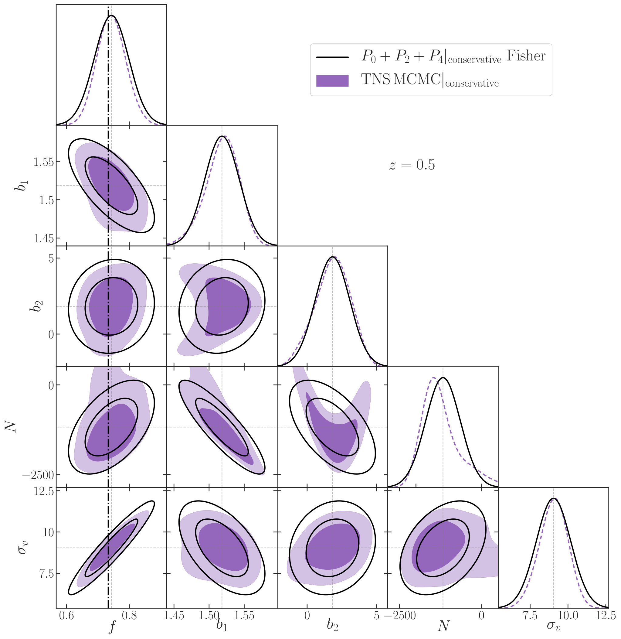 Figure 1
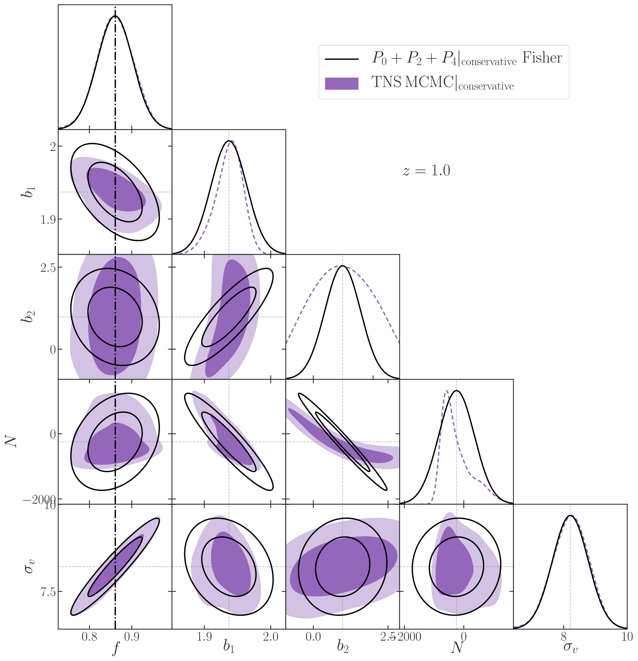 Figure 2
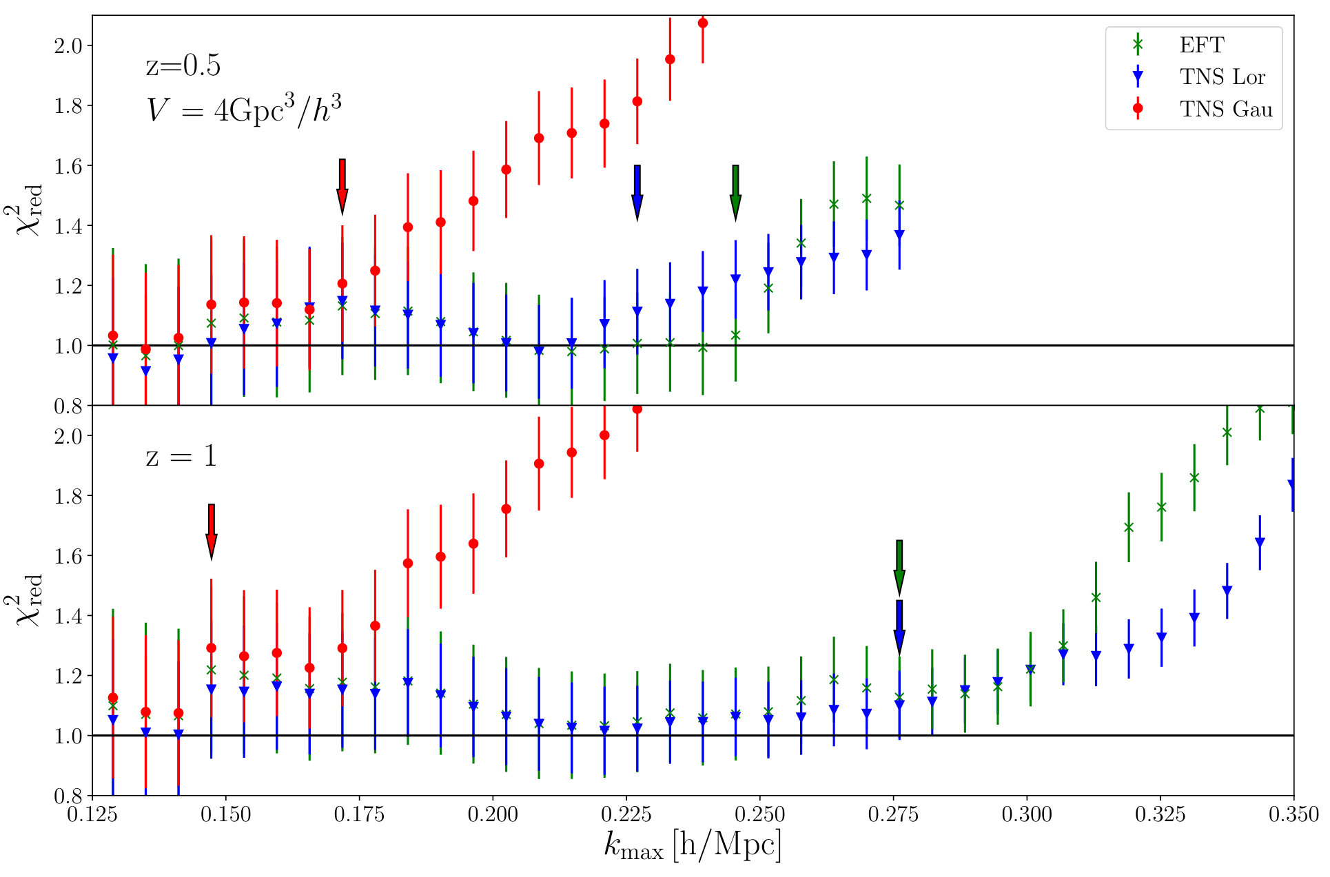 Figure 3
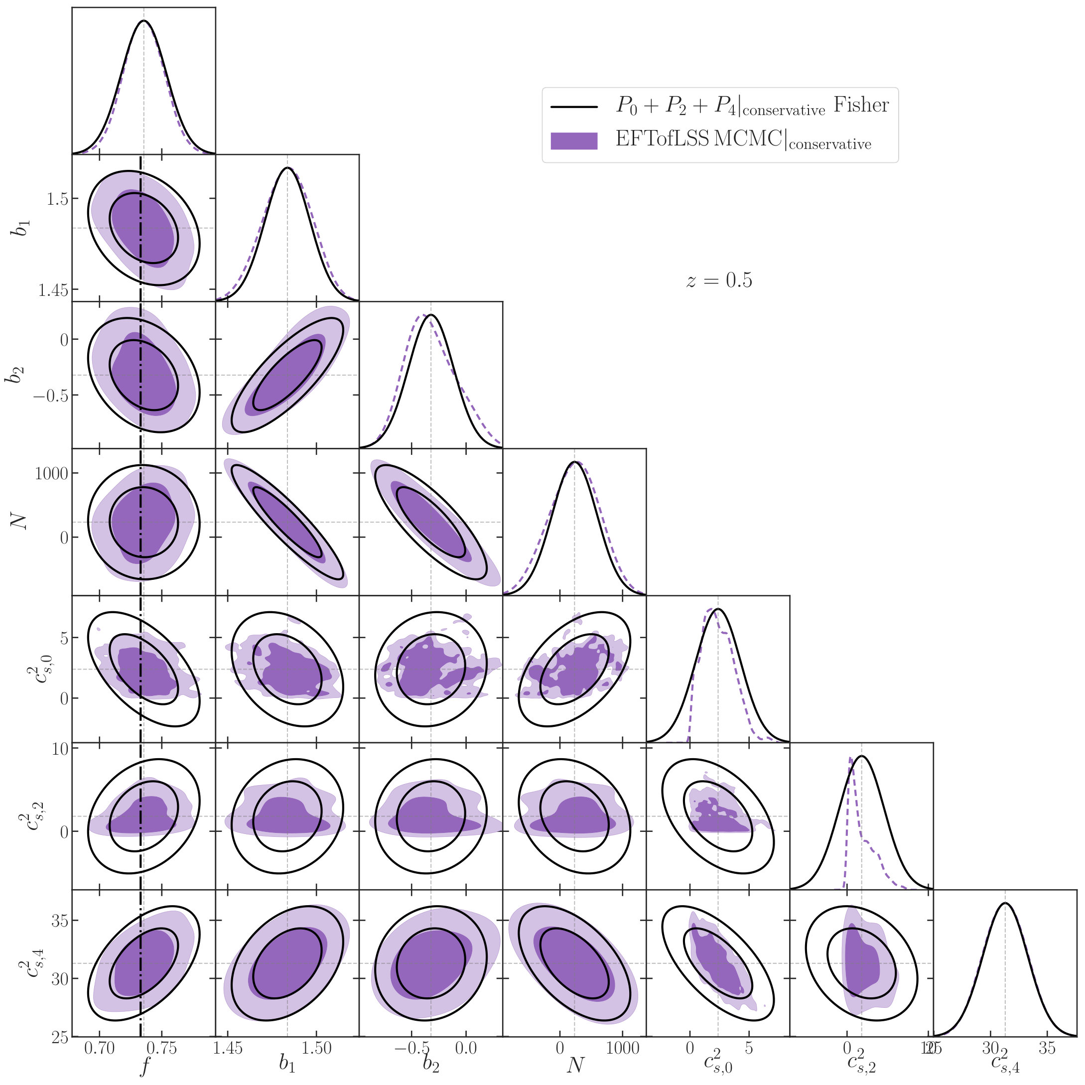 Figure 4
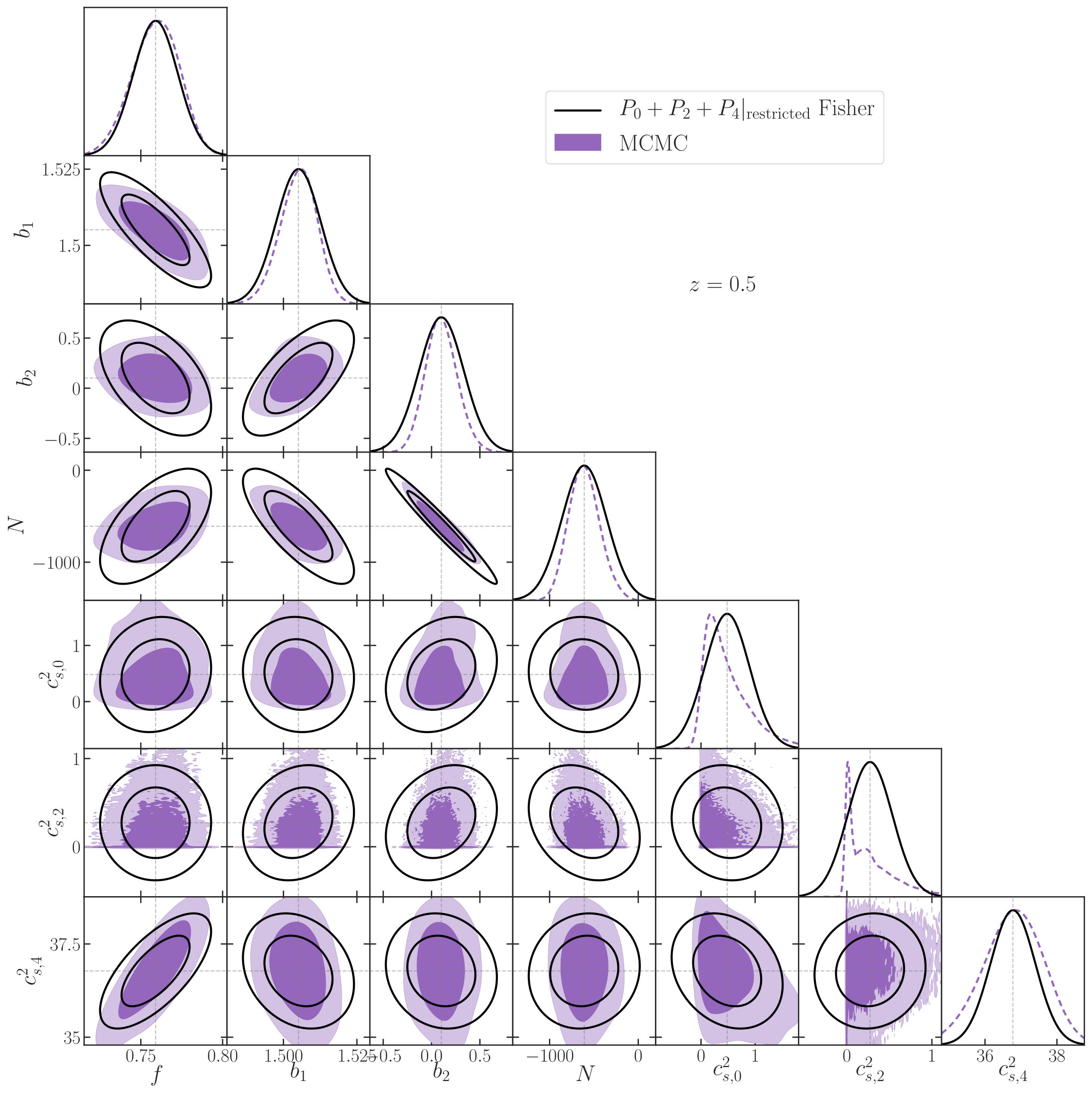 Figure 5
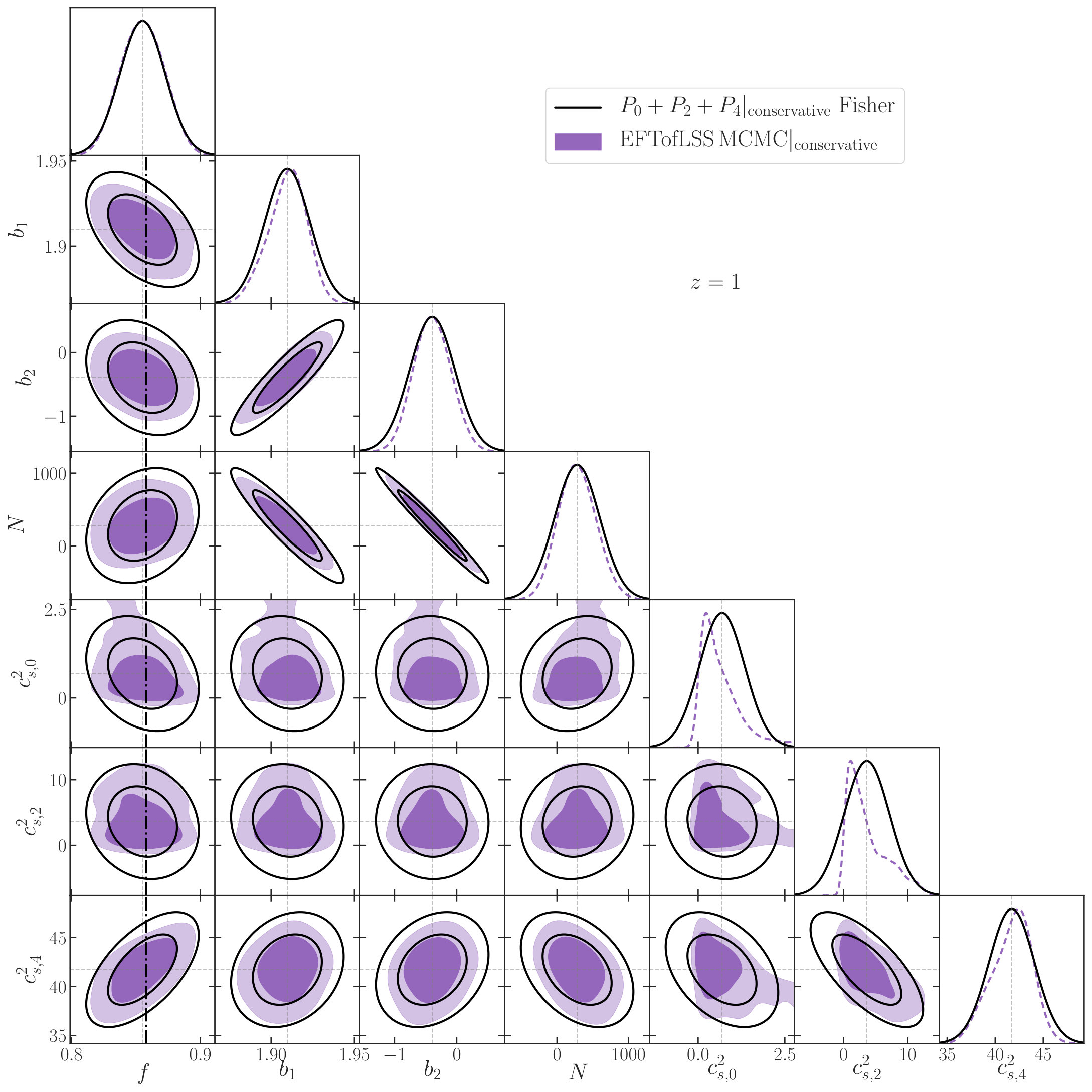 Figure 6
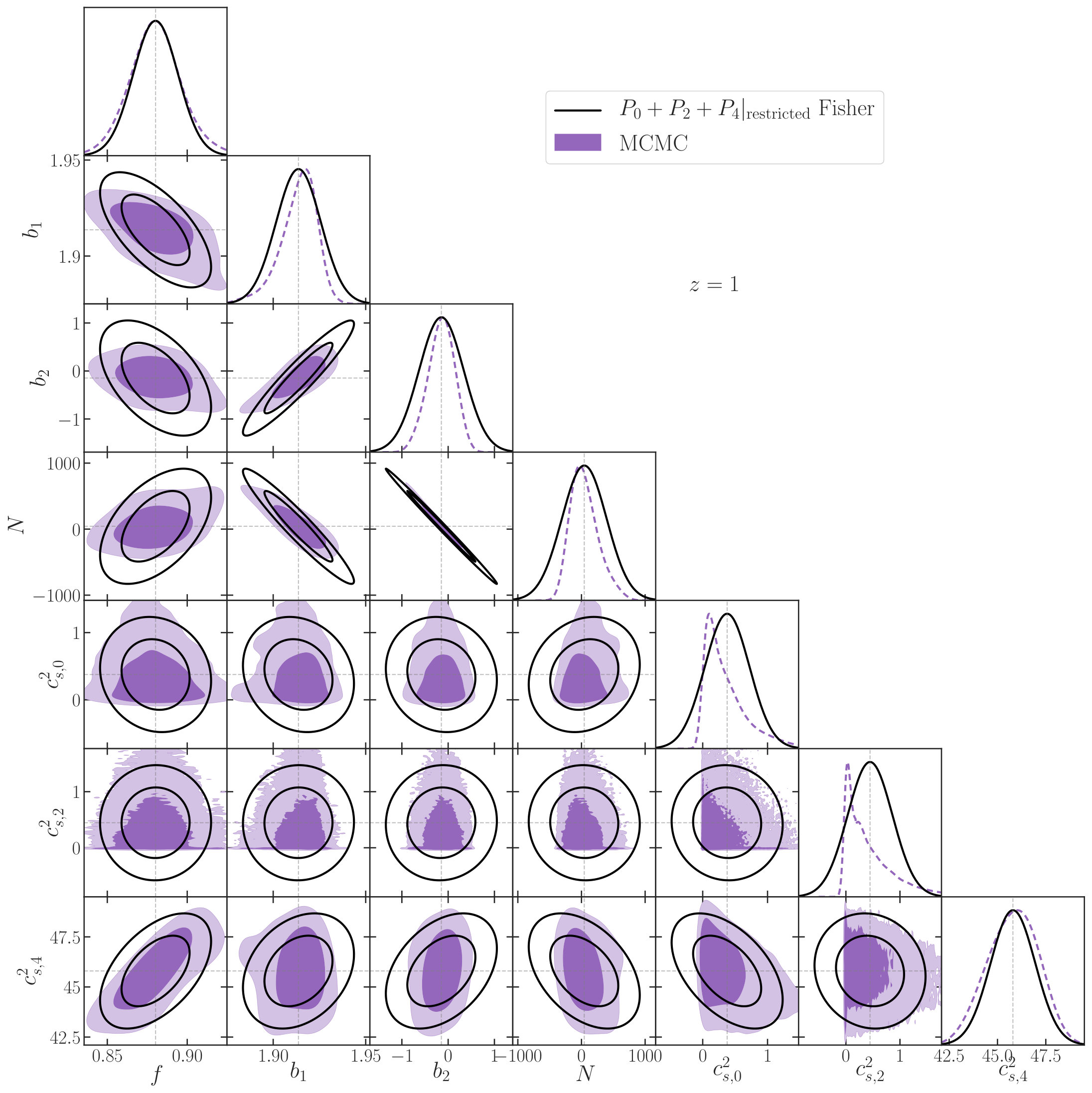 Figure 7
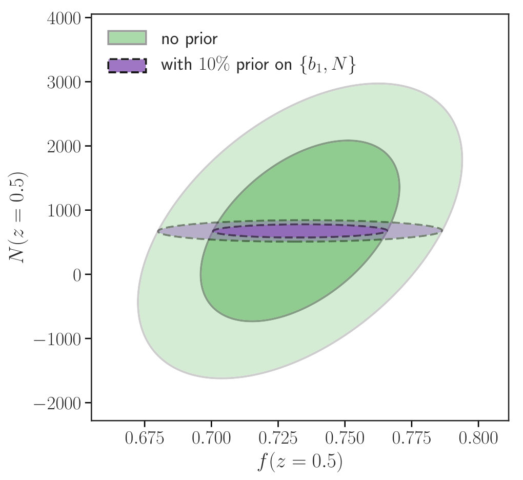 Figure 8
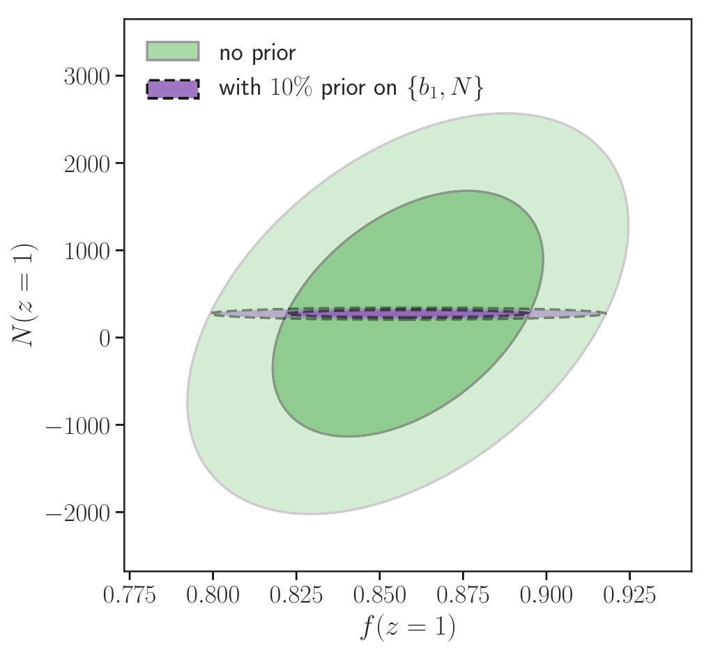 Figure 9
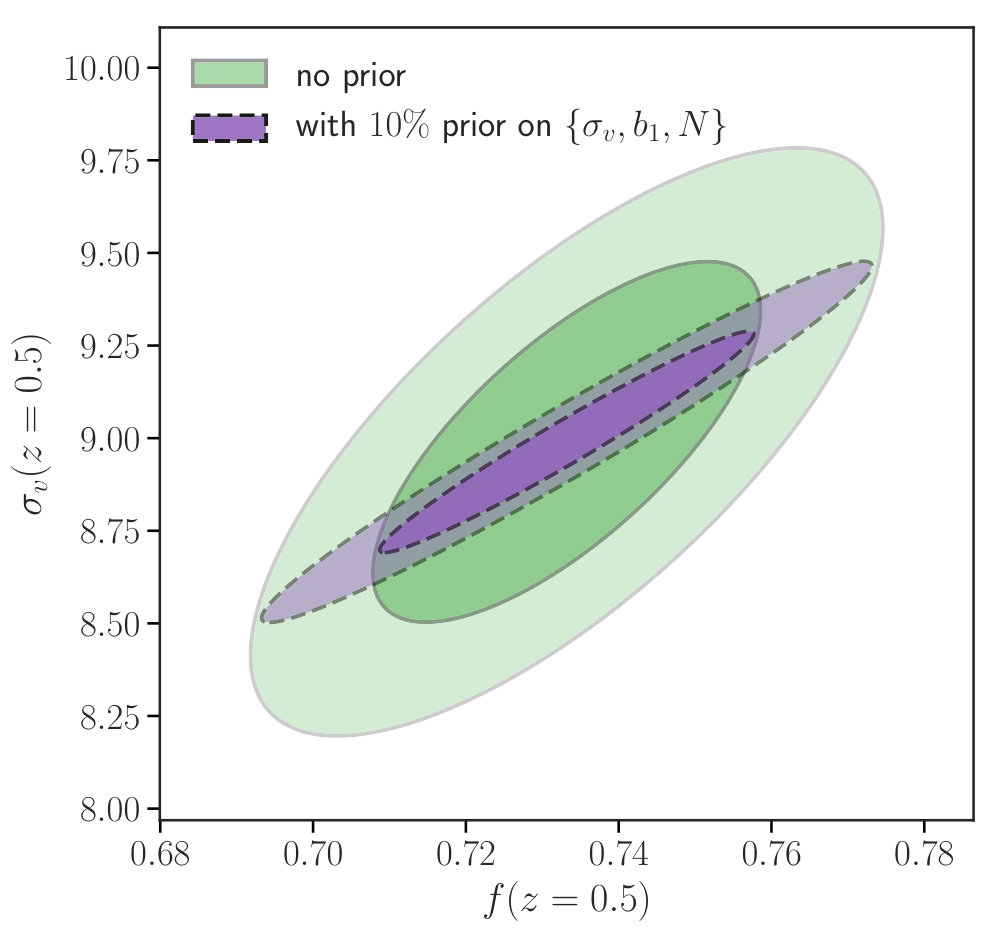 Figure 10
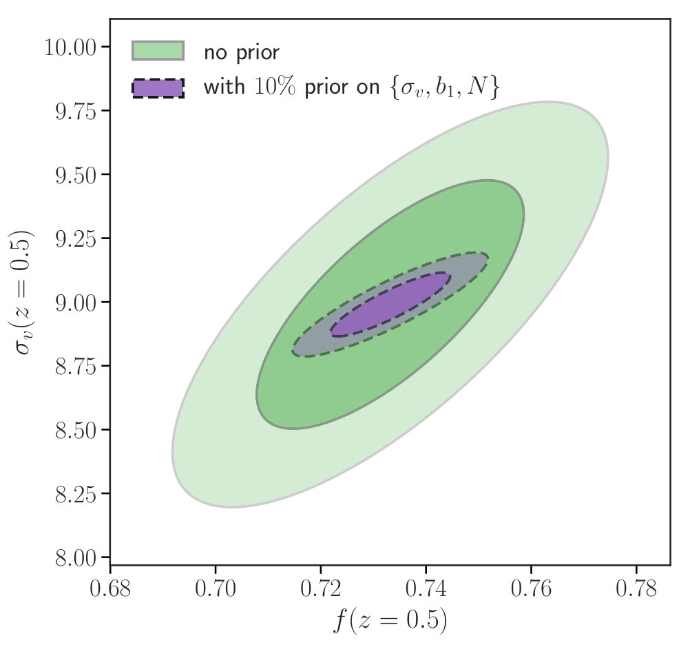 Figure 11
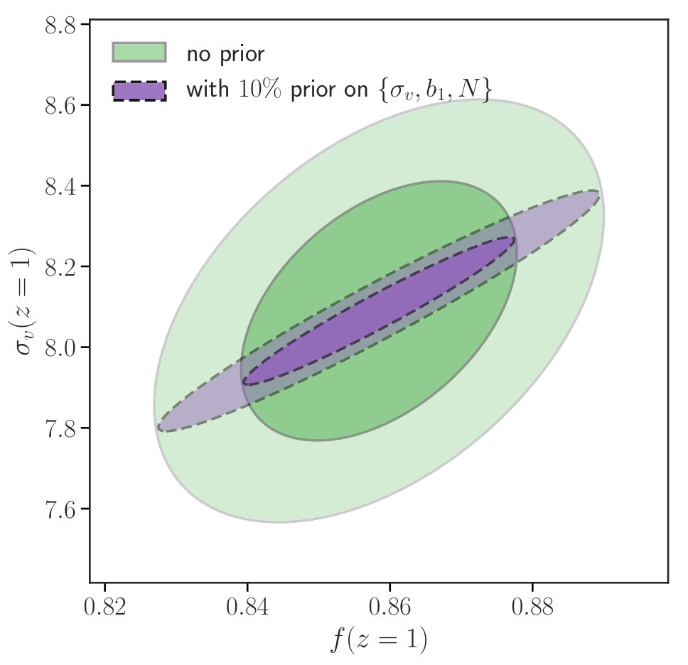 Figure 12
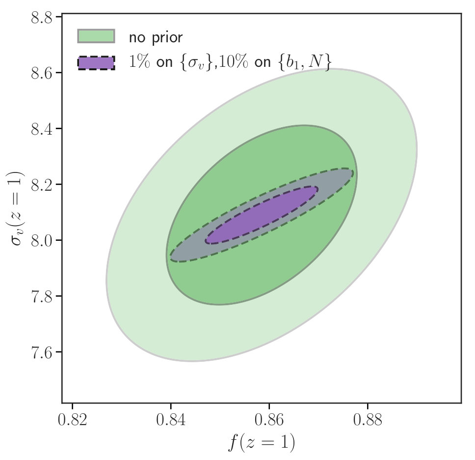 Figure 13
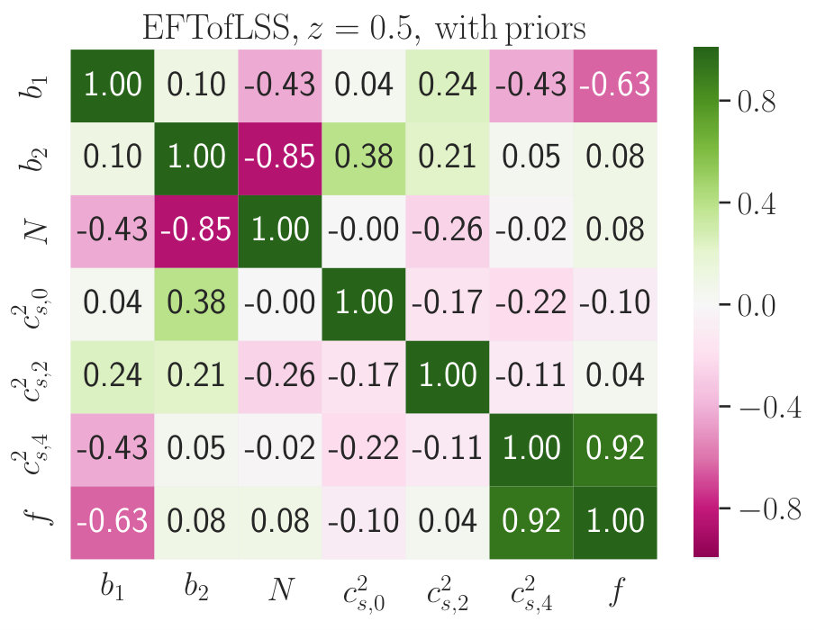 Figure 14
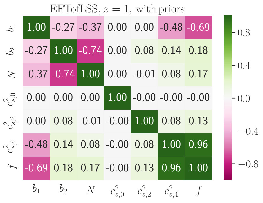 Figure 15
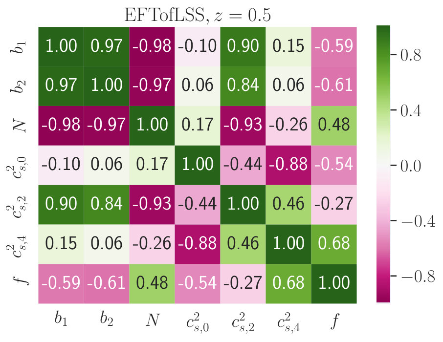 Figure 16
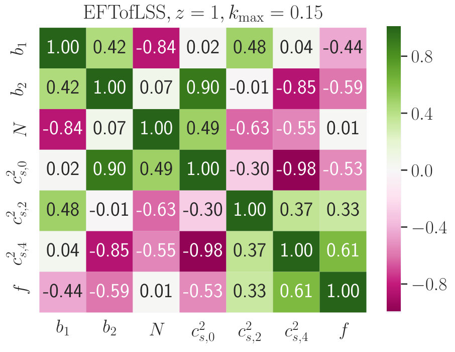 Figure 17
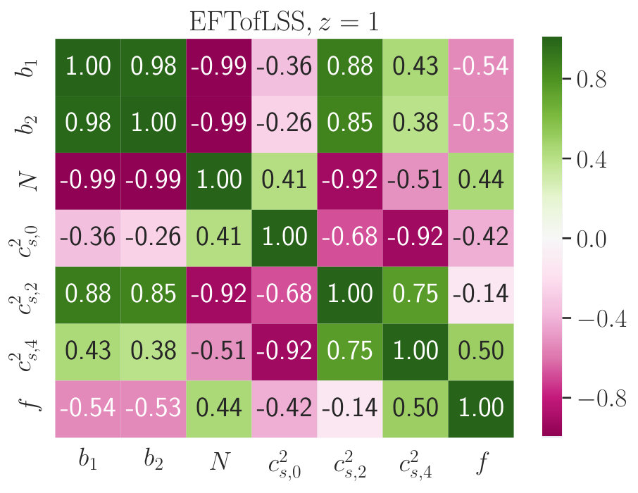 Figure 18
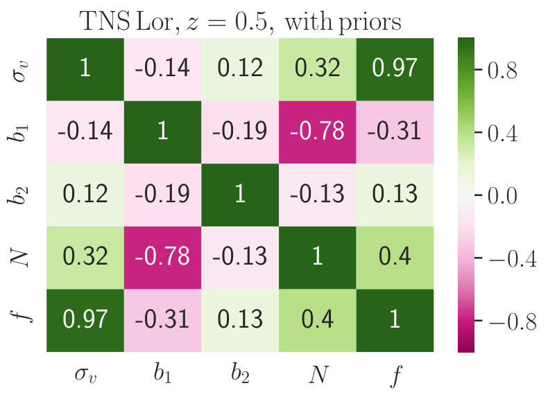 Figure 19
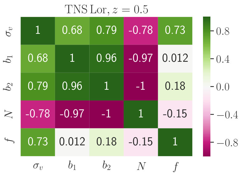 Figure 20
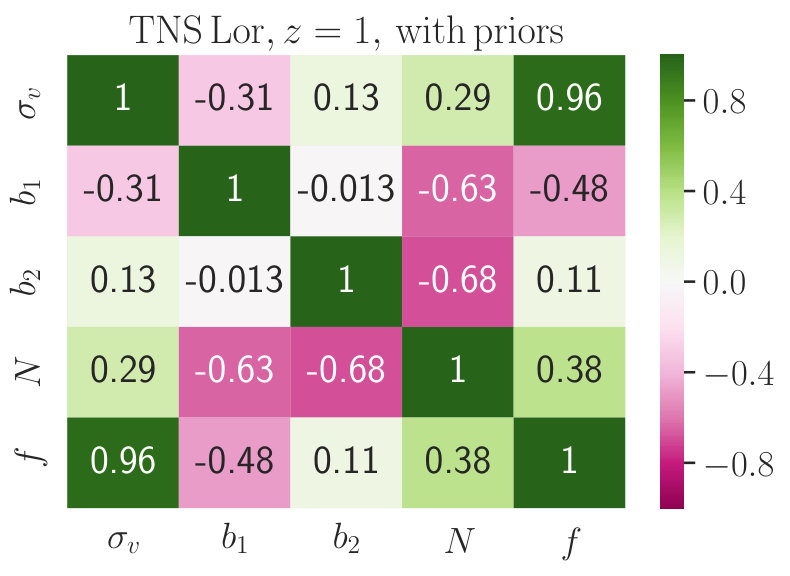 Figure 21
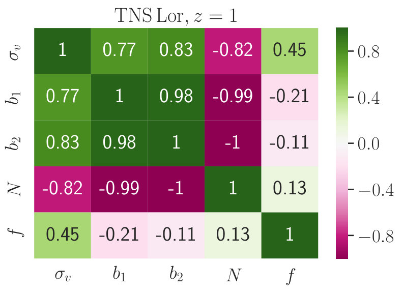 Figure 22
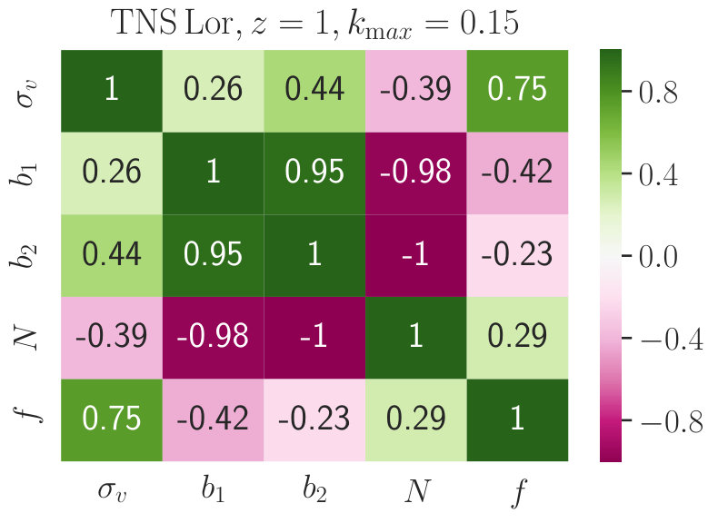 Figure 23
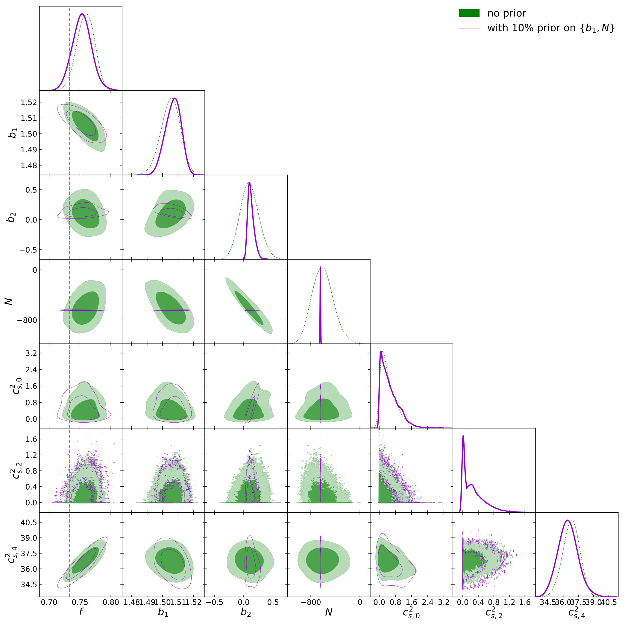 Figure 11
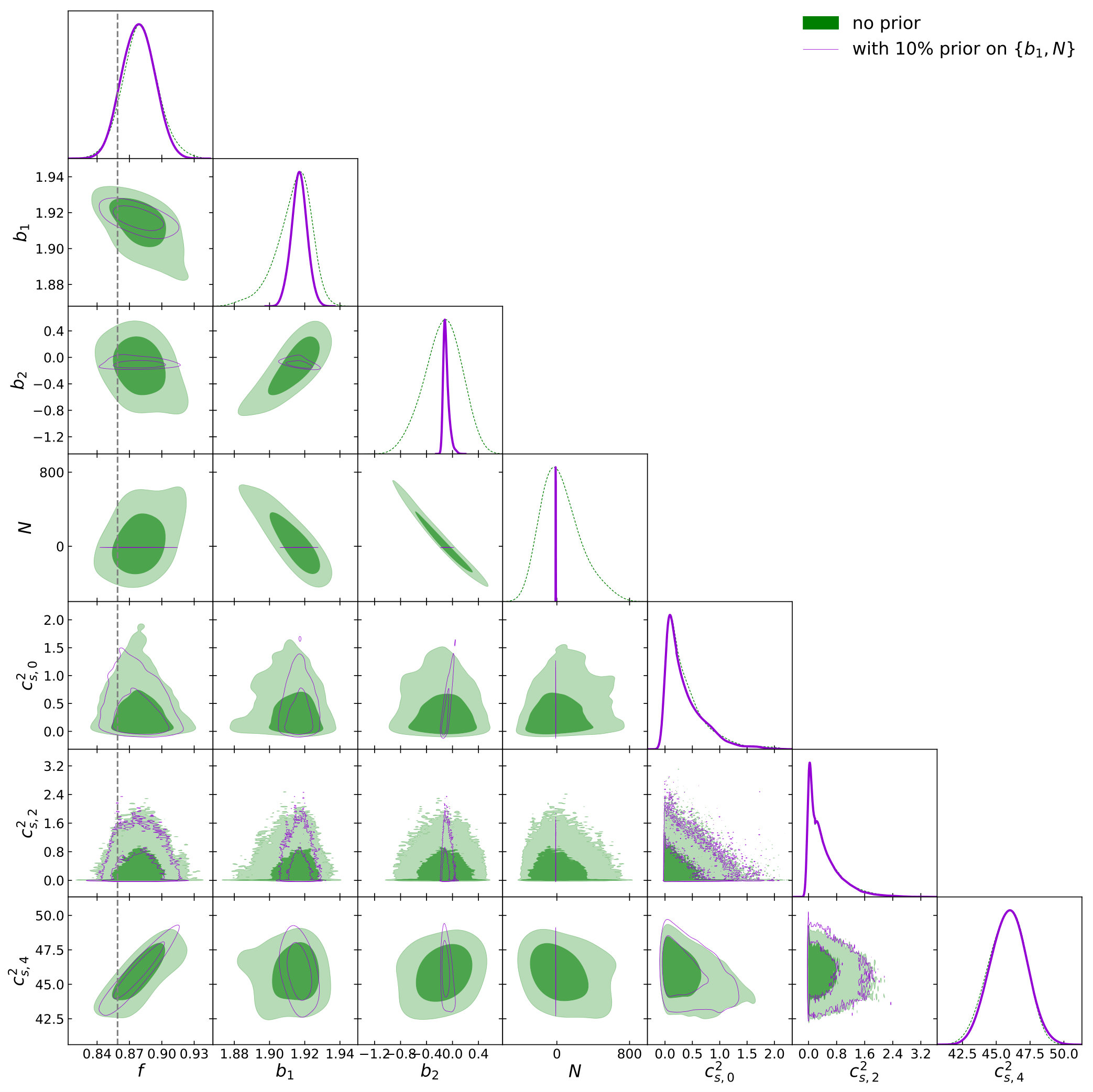 Figure 13
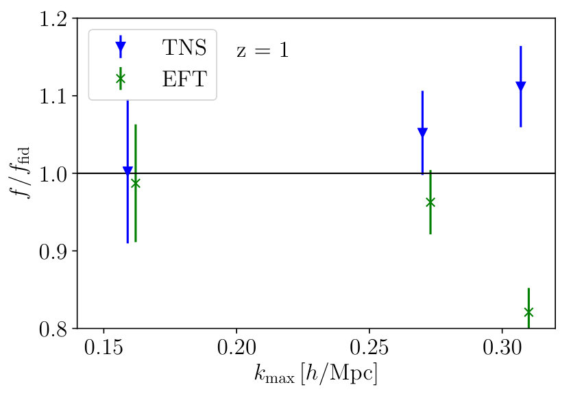 Figure 26
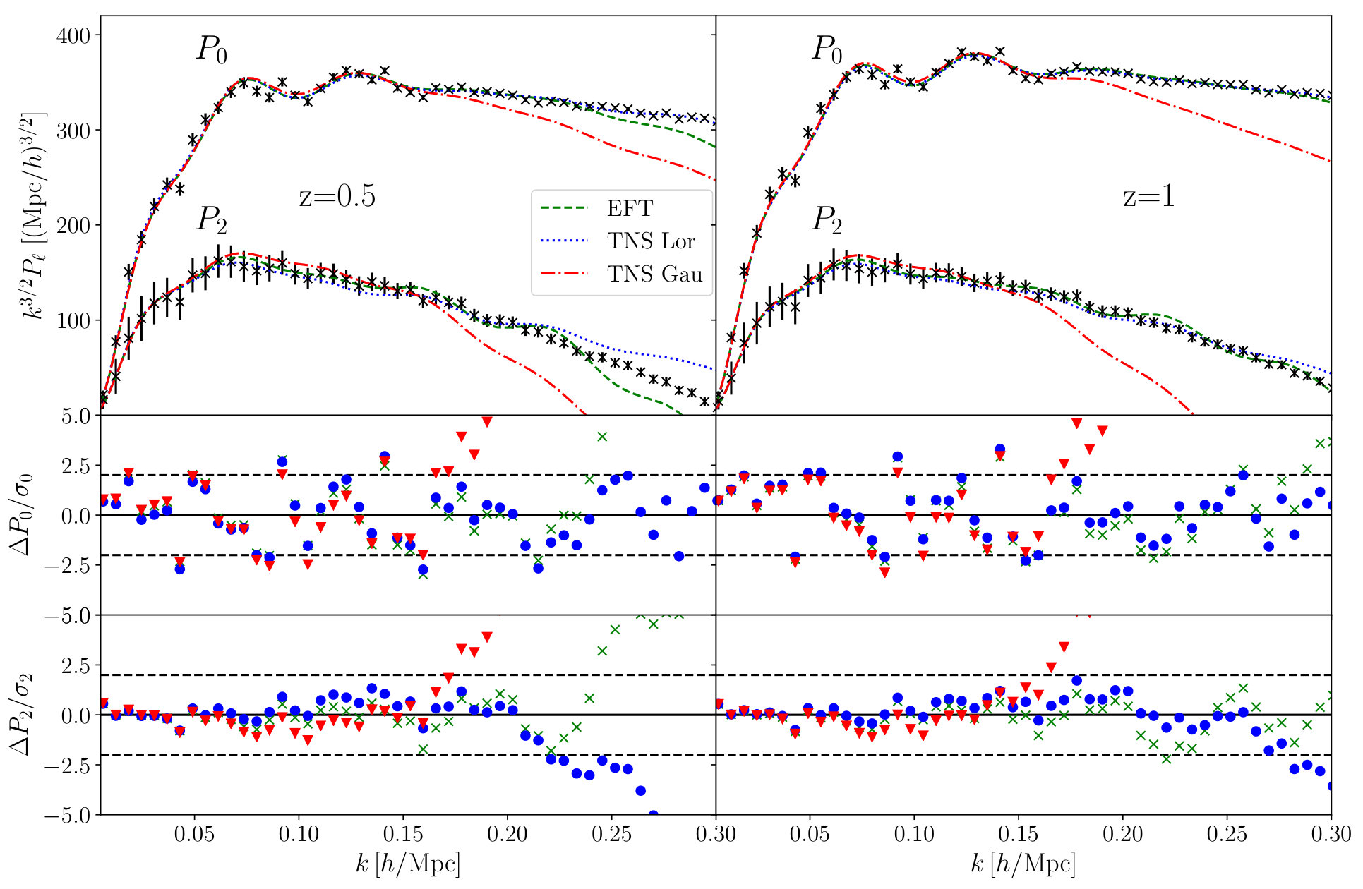 Figure 27
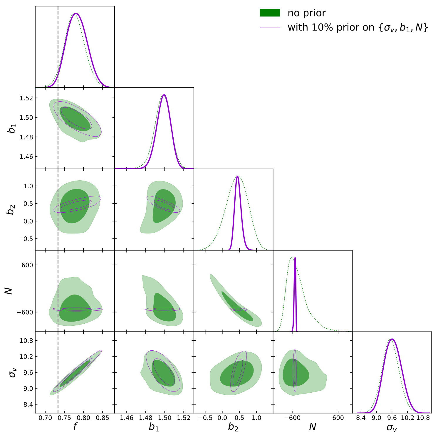 Figure 28
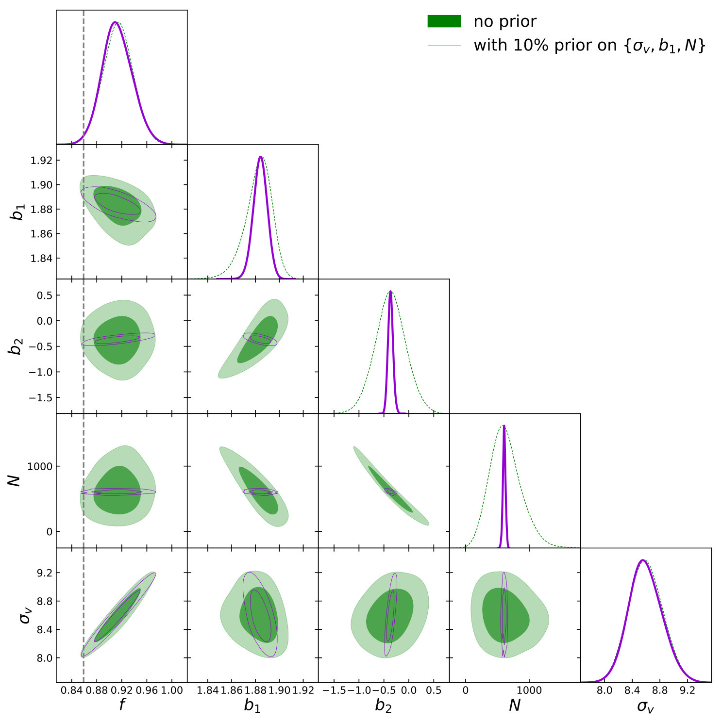 Figure 29
| Model | TNS Lor | TNS Gau | EFTofLSS | |||
| z | ||||||
| - | - | |||||
| - | - | - | - | |||
| - | - | - | - | |||
| - | - | - | - | |||
| TNS-based model | EFTofLSS-based model | ||
|---|---|---|---|
| + prior | |||
| + prior | |||
| TNS Lor | EFTofLSS | |||||
|---|---|---|---|---|---|---|
| prior | prior | |||||
| 0.5 | ||||||
| 1 | ||||||
Peer Reviews
No public reviews on file for this paper yet. If you reviewed it on a platform where reviews are public (OpenReview, ICLR, NeurIPS, ICML), you can paste yours below so the community can read it here.
Code & Models
Videos
No videos yet. Explain this paper in a talk, walkthrough, or lecture? Add one.
Assessing non-linear models for galaxy clustering II: model validation and forecasts for Stage IV surveys
Benjamin Bose1, Alkistis Pourtsidou2,3, Katarina Markovič4,5, Florian Beutler4
1Departement de Physique Theorique, Universite de Geneve, 24 quai Ernest Ansermet, 1211 Geneve 4, Switzerland
2School of Physics and Astronomy, Queen Mary University of London, Mile End Road, London E1 4NS, UK
3Department of Physics & Astronomy, University of the Western Cape, Cape Town 7535, South Africa
4Institute of Cosmology & Gravitation, University of Portsmouth, Dennis Sciama Building, Burnaby Road, Portsmouth PO1 3FX, UK
5Jet Propulsion Laboratory, California Institute of Technology, 4800 Oak Grove Drive, Pasadena, CA 91109, USA E-mail:[email protected]
(Accepted XXX. Received YYY; in original form ZZZ)
Abstract
Accurate modelling of non-linear scales in galaxy clustering will be crucial for data analysis of Stage IV galaxy surveys. A selection of competing non-linear models must be made based on validation studies. We provide a comprehensive set of forecasts of two different models for the halo redshift space power spectrum, namely the commonly applied TNS model and an effective field theory of large scale structure (EFTofLSS) inspired model. Using simulation data and a least- analysis, we determine ranges of validity for the models. We then conduct an exploratory Fisher analysis using the full anisotropic power spectrum to investigate parameter degeneracies. We proceed to perform an MCMC analysis utilising the monopole, quadrupole, and hexadecapole spectra, with a restricted range of scales for the latter in order to avoid biasing our growth rate, , constraint. We find that the TNS model with a Lorentzian damping and standard Eulerian perturbative modelling outperforms other variants of the TNS model. Our MCMC analysis finds that the EFTofLSS-based model may provide tighter marginalised constraints on at and than the TNS model, despite having additional nuisance parameters. However this depends on the range of scales used as well as the fiducial values and priors on the EFT nuisance parameters. Finally, we extend previous work to provide a consistent comparison between the Fisher matrix and MCMC forecasts using the multipole expansion formalism, and find good agreement between them.
keywords:
cosmology: theory – large-scale structure of the Universe – methods: analytical
††pubyear: 2019††pagerange: Assessing non-linear models for galaxy clustering II: model validation and forecasts for Stage IV surveys–References
1 Introduction
The standard model of cosmology, CDM, has been hugely successful in reproducing many cosmological observations such as the cosmic microwave background (CMB) (Ade et al., 2016) and the large scale structure of the universe (LSS) (Anderson et al., 2013; Song et al., 2015; Beutler et al., 2017). The model relies on two fundamental theoretical assumptions: that general relativity holds on all physical scales and that the universe is homogeneous and isotropic on large scales. While CDM fits observational data extremely well, it requires the introduction of two exotic dark components: cold dark matter (CDM) and dark energy in the form of a cosmological constant (), which account for of the matter-energy content of the Universe today. Probing the nature of dark matter and dark energy is a key driver in modern cosmology, and a plethora of dark matter, exotic dark energy and modified gravity models have been proposed (for respective reviews, see Bertone et al., 2005; Copeland et al., 2006; Clifton et al., 2012).
Large scale structure (LSS) measurements offer promising means of testing CDM and gravity. In particular, the measurement of the redshift space distortions (RSD) phenomenon in the galaxy distribution can put meaningful constraints on cosmology. This has traditionally been done by modeling the redshift space galaxy power spectrum or correlation function (Blake et al., 2011; Reid et al., 2012; Macaulay et al., 2013; Beutler et al., 2014; Gil-Marín et al., 2016a; Simpson et al., 2016). It is expected that very precise measurements of the observables will be made with the commencement of new, very large spectroscopic surveys such as EUCLID111www.euclid-ec.org (Blanchard et al., 2019), WFIRST222https://wfirst.gsfc.nasa.gov/, the Dark Energy Spectroscopic Instrument (DESI)333www.desi.lbl.gov (Aghamousa et al., 2016), and the Square Kilometre Array (SKA)444www.skatelescope.org/ (Bacon et al., 2018).
In order to make the most of the upcoming data sets, theoretical models for the redshift space galaxy power spectrum must be studied carefully. Perturbation theory based models offer a robust and computationally quick means of modeling the RSD at large distance scales (Bernardeau et al., 2002; Kaiser, 1987; Scoccimarro, 2004). Furthermore, they offer the flexibility to give predictions for a wide range of gravity and dark energy models (Bose & Koyama, 2016, 2017; Bose et al., 2018a; Bose et al., 2018b). To extend their range of applicability, phenomenological ingredients can be added in order to model non-linear physics (Taruya et al., 2010; Senatore & Zaldarriaga, 2014; de la Bella et al., 2017). Working in Fourier space and assuming a high degree of Gaussianity, the amount of information available in the matter power spectrum is roughly given by the number of independent modes we can access. Therefore, extending theoretical models to include non-linear scales should in principle allow us to extract much more information from data. However, this is heavily dependent on our ability to model non-linear structure formation in an unbiased way.
On top of this, additional modeling is required to relate the dark matter and galaxy distributions, a relation called galaxy bias. Such non-linear and galaxy bias modeling often come with so-called ‘nuisance’ parameters, which are not known (up to some motivated priors) a priori. As their name implies, these parameters are not generally interesting and are marginalized over when constraining cosmology. This marginalization weakens our constraints, essentially leading us to an issue of optimization. We then must ask: What models give us an accurate description of the galaxy distribution over the largest range of scales but without invoking unnecessary degrees of freedom? The issue of optimal power spectrum modeling has been recently studied in a number of works (de la Bella et al., 2018; Osato et al., 2019; Bose et al., 2018b) and will be the focus of this paper.
At the current forefront of perturbation theory based RSD modeling are two main approaches. The first is the so-called TNS model (Taruya et al., 2010), which combined with the bias model of McDonald & Roy (2009) has been an integral part of the BOSS data analysis (Beutler et al., 2017). This model has been studied extensively and has been shown to reproduce the broadband power spectrum including RSD from simulations at linear and moderately non-linear scales (Nishimichi & Taruya, 2011; Taruya et al., 2013; Ishikawa et al., 2014; Zheng & Song, 2016; Gil-Marín et al., 2016a, b; Bose et al., 2017; Bose & Koyama, 2016; Markovic et al., 2019).
The second is the effective field theory approach (EFT) commonly used in other fields of physics such as particle physics or condensed matter. The EFT of LSS (EFTofLSS) (Baumann et al., 2012; Carrasco et al., 2012) represents an attempt to separate linear and non-linear physics so that one can safely model contributions from the small scale regime independently from the large scale contributions, as well as any back-reaction effects by the non-linear physics on the linear scales. The non-linear modeling comes with degrees of freedom in the form of sound speed parameters . These parameters are time dependent coupling constants that arise from treating the stress energy tensor perturbatively and performing a time integral over the Green’s function and associated kernels in order to get the corresponding contributions to the power spectrum. This approach has been shown to model simulation measurements down to much smaller scales than the standard perturbative approach (Senatore & Zaldarriaga, 2014; Lewandowski et al., 2018; Perko et al., 2016; Foreman et al., 2016) and has become a promising means of modeling LSS. Recent bias models have also been developed within this framework (Angulo et al., 2015; Perko et al., 2016; Fujita et al., 2016) but these generally come with many additional degrees of freedom. For example Perko et al. (2016) models the RSD halo power spectrum with 10 nuisance parameters.
In this work we consider a TNS-based model similar to that used in the BOSS survey (Beutler et al., 2017) and one of the EFTofLSS-based models used in de la Bella et al. (2018), but with a reduced nuisance parameter set. Using a set of COLA simulations (Tassev et al., 2013; Howlett et al., 2015; Valogiannis & Bean, 2017; Winther et al., 2017) we determine a range of validity for the models555 We have checked that the deviation of COLA from full N-body is sufficiently accurate for the scales of interest for the halo monopole we utilise in this work.. We then perform an exploratory Fisher matrix forecast analysis using the full anisotropic power spectrum and specifications similar to forthcoming Stage IV spectroscopic surveys. The Fisher analysis allows the fast exploration of parameter space and the fast investigation of different assumptions. We focus on investigating parameter degeneracies and the effect of imposing priors on nuisance parameters, as well as providing estimates for the constraints we can expect on the logarithmic growth rate, . This parameter is strongly cosmology and gravity dependent, and represents the rate at which structure grows in a Friedman-Lemaitre-Robertson-Walker universe. We proceed to present various MCMC analyses which provide a more accurate test of parameter degeneracies and marginalised constraints. We finally follow previous studies (Wolz et al., 2012; Hawken et al., 2012) and compare our EFTofLSS posterior probability distributions resulting from MCMC to that of the Fisher analysis. We conduct the analysis using power spectrum multipoles, , in order to make it maximally comparable to real data analysis, as we recommended in Paper I of this series (Markovic et al., 2019).
This paper is organized as follows: In section 2 we present the biased tracer RSD models. In section 3 we present a comparison of model predictions with simulation data and determine fiducial nuisance parameters and a range of validity for each. In section 4 we perform the exploratory Fisher analysis with our chosen models and present results, followed by the MCMC analysis and results in section 5. In section 6 we perform a comparison between Fisher matrix and MCMC forecasts using the multipole expansion formalism. In section 7 we summarise our findings and conclude.
2 Theoretical background and model selection
We begin by presenting the two models we will use in our forecasts. Both are based on standard Eulerian perturbation theory (SPT), which has the following core assumptions:
- •
We live on a spatially expanding, homogeneous and isotropic background spacetime.
- •
We work on scales far within the horizon but at scales where , where and are the density and velocity perturbations respectively. This is the so called Newtonian regime at quasi non-linear scales.
In addition we assume that the gravitational interaction is described by general relativity 666This assumption can be relaxed quite easily within SPT (e.g Bose & Koyama, 2016).. Aside from the above, each model includes phenomenological ingredients and a set of free parameters which will be made explicit in the following sections.
2.1 TNS-based model
The first is the TNS RSD model (Taruya et al., 2010) combined with the tracer bias model of McDonald & Roy (2009). A similar model has been used in the BOSS analyses to infer cosmological constraints (Beutler et al., 2014, 2017), the exact differences from which will be made explicit soon. The model is given by
[TABLE]
where the superscript denotes the power spectrum in redshift space. The terms in brackets are all constructed within SPT, while the prefactor, , is added for phenomenological modeling of the fingers-of-god effect. Within this prefactor, is a free parameter and represents the velocity dispersion of the cluster; is the logarithmic growth rate and is the cosine of the angle between and the line of sight. The perturbative components of the model, along with the explicit dependency on the linear bias , second order bias and constant stochasticity nuisance parameters, are given by 777We make the local Lagrangian bias assumption (Sheth et al., 2013; Chan et al., 2012; Saito et al., 2014; Baldauf et al., 2012).
[TABLE]
where is the linear growth factor at the desired redshift and is the primordial matter power spectrum. Note that there is no velocity bias, therefore .The 1-loop dark matter spectra are then given by
[TABLE]
where and and . The components are further expanded in terms of the standard Einstein-de Sitter perturbative kernels and (Bernardeau et al., 2002) as
[TABLE]
and
[TABLE]
The RSD correction terms, , and are given by
[TABLE]
where \mu_{p}=\hat{\mbox{\boldmathk}}\cdot\hat{\mbox{\boldmathp}}, and x=\hat{\mbox{\boldmathk}}\cdot\hat{\mbox{\boldmathq}}. Explicit expressions for and can be found in the Appendices of Taruya et al. (2010). The term is known to have small enough acoustic features so it is usually omitted in the literature. It can be effectively absorbed into the fingers-of-god prefactor of Equation 1. In our analysis we include it. Finally, the bias terms are given by
[TABLE]
where the additional kernel is given by
[TABLE]
where is the cosine of the angle between \mbox{\boldmathq}_{1} and \mbox{\boldmathq}_{2}. Since we only consider moderately non-linear scales and redshifts at or above , where non-linearity is weak, the following assumptions we have made are valid:
Negligible velocity bias, i.e. . 2. 2.
The local Lagrangian assumption (as validated by N-body simulations, Baldauf et al., 2012). This allows us to reduce the number of free bias parameters from 5 to 3. 3. 3.
The Einstein-de Sitter approximation in the perturbative calculations allowing us to separate time and scale components of the perturbations. This is well known to be an excellent approximation for GR (Bose & Koyama, 2016; Bose et al., 2018b).
Furthermore, we will investigate two functional forms for the term, a Lorentzian and a Gaussian:
[TABLE]
The key differences between this model and that used in the galaxy clustering data analysis of Beutler et al. (2017) for example, is the inclusion of the term and the fact that we use SPT instead of the RegPT prescription of Taruya et al. (2012) for the 1-loop dark matter power spectra (Equation 4). In that analysis they choose the Gaussian form for . Furthermore, the TNS model is similar to the M&R+SPT model considered in de la Bella et al. (2018). In that model they only consider the Gaussian damping factor shown above and do not assume the local Lagrangian picture. Further, they exclude , giving their bias model degrees of freedom. We choose instead to use the bias model as used in the BOSS analysis in Beutler et al. (2017).
The full set of nuisance parameters in the TNS-based model we use is therefore .
2.2 EFTofLSS-based Model
The second model we consider is based on the EFTofLSS prescription for the redshift space dark matter spectrum (de la Bella et al., 2017) given by
[TABLE]
where are the sound speed parameters of EFTofLSS and indicates the strong coupling scale. None of these can be calculated, so they are usually measured as the combination . The is the 1-loop SPT prediction for the redshift space power spectrum. As in de la Bella et al. (2017), a resummation technique (Vlah et al., 2016) is applied to the 1-loop spectra. The is almost identical to Equation 1 with , and the phenomenological exponential prefactor now given by the SPT prediction , where
[TABLE]
Also note that this prefactor does not multiply the correction terms , and (see Equation 1).
The power spectrum model suggested here simply upgrades the redshift space dark matter spectrum to a biased tracer spectrum by using the bias model of McDonald & Roy (2009). In this way we are only really adding EFTofLSS-like counter terms (terms involving ) to the SPT predicted redshift space halo spectrum. This model is very similar to the EFT+M&R model considered in de la Bella et al. (2018) with the difference that we omit the stochastic EFTofLSS terms that introduce an additional 3 nuisance parameters. The explicit expression is
[TABLE]
where we have absorbed the into the . We can motivate Equation 26 by arguing that the bias is well described by the McDonald & Roy (2009) model and we are just missing a suppression of power coming from small cosmological scales that can be described by the dark matter EFTofLSS counter-terms. Before proceeding we make two comments on the model proposed here.
First, we have omitted the 3 stochasticity terms of the EFTofLSS redshift space spectrum (Baumann et al. (2012); Lewandowski et al. (2018)). For the dark matter power spectrum, these terms go as and hence are not expected to impact the predictions at the scales considered here. This was also investigated and confirmed in the analysis of de la Bella et al. (2017). For halos, the omission of the stochastic terms may have an effect on the fits, but as we are making the assumption that all bias physics is captured by the McDonald & Roy (2009) model, we do not consider them. Further, the most that these terms can improve the range of validity of the model is up to the regime where the 2-loop contributions become important (Carrasco et al., 2014). This extension in scale is not expected to compensate the degradation of marginalised constraints from the inclusion of 3 additional parameters – this could be checked but is not the focus of this work. For a complete treatment of bias within the EFTofLSS we direct the reader to Perko et al. (2016). This treatment comes with free parameters and given the Bayesian information criterion used in de la Bella et al. (2018) it is unlikely to be favoured against a similar model with fewer free parameters.
Second, we have not performed a full infra-red resummation of the baryon acoustic oscillation features, but rather have only applied resummation to the 1-loop power spectra pieces in Equation 26. Since we have checked that there are large biases in the prediction for incurred by increasing beyond the determined values, we do not expect inaccuracies in the resummation applied to improve this validity range for the model. Further, in de la Bella et al. (2018), the authors find that the exclusion of resummation in a model very similar to that proposed here does not affect their fits to simulations.
The full set of nuisance parameters in the EFTofLSS-based model we use is therefore . This is an additional 2 parameters compared to the TNS approach described by Equation 1.
In Equation 1 and Equation 26 we can immediately see the dependency of the power spectrum on the model parameters. The logarithmic growth rate, is also explicit. Cosmological parameter dependence enters through the primordial power spectrum with 888 governs the amplitude of density perturbations at Mpc/. being completely degenerate with . For our analysis in the next section, since we are focused on comparing the power spectrum models, we assume a CDM expansion and fix cosmology as well as and to their known values.
3 Comparison to simulations
In this section we determine fiducial values for the nuisance parameters of each model described in the previous section as well as their respective ranges of validity. This is done by comparing to a set of Parallel COmoving Lagrangian Acceleration (PICOLA) simulations (Howlett et al., 2015; Winther et al., 2017). Specifically, we use a set of four CDM simulations of box length with dark matter particles and a starting redshift . The summed volume of these realisations is similar to Stage IV surveys such as DESI and Euclid at for a bin width of (Aghamousa et al., 2016; Majerotto et al., 2012).
The background cosmology in these DM-only simulations is taken from WMAP9 (Hinshaw et al., 2013): , , , and and . We use halo catalogs, which were constructed using the friends-of-friends algorithm with a linking length of 0.2-times the mean particle separation. We consider the redshifts and . For our analysis we use all halos above a mass of . We note that the mass cut choice will affect the fiducial values and range of validity, and so we base our choice on the corresponding number density of halos at this mass cut which is . This number density is similar to that estimated for Stage IV surveys galaxy number density around the redshifts considered.
To determine the fiducial values of the parameters and ranges of validity for the models we perform a fit to the simulated data using the redshift space power spectrum multipoles. PICOLA multipoles are measured using the distant-observer approximation999That is, we assume the observer is located at a distance much greater then the box size (), so we treat all the lines of sight as parallel to the chosen Cartesian axes of the simulation box. Next, we use an appropriate velocity component ( or ) to disturb the position of a matter particle. and averaged over three line-of-sight directions. We further average over the four PICOLA simulations.
On the theoretical side, the multipoles are defined as
[TABLE]
where denote the Legendre polynomials and is given by Equation 1 or Equation 26. For our fitting analysis, we utilise only the monopole () and quadrupole (). The inclusion of the hexadecapole would significantly restrict the determined range in scale of validity and consequently the information gained since the monopole and quadrupole contain most of the RSD information. It is later considered in section 5, where we perform an MCMC analysis on the PICOLA data.
To determine the range of validity, , that will be used to determine the fiducial parameters for each model, we follow the procedure outlined below:
We fix all cosmological parameters including the growth rate and perform a least-squares fit to the PICOLA data by varying the model nuisance parameters. We do this for all data bins within . 2. 2.
We take the () confidence intervals () on a distribution with degrees of freedom. Since is large in our analysis the errors are approximately symmetric. 3. 3.
We determine as the maximum k-value which has .
This gives a fair indication of the point at which the model gives a good fit to the data without biasing cosmology estimates101010We test this by performing an MCMC analysis with being allowed to vary at the determined here. For the TNS case, see Paper I.. The reduced statistic is given by
[TABLE]
where is the Gaussian covariance matrix between the different multipoles and . The number of degrees of freedom is given by , where is the number of bins used in the summation and is the number of free parameters in the theoretical model. Here, for the TNS model of Equation 1, and for the EFTofLSS model of Equation 26. The is not for the EFTofLSS model because we only consider the monopole and quadrupole. When integrating to get each of these two multipoles, they come with the same k-dependent piece, , multiplied by a different linear combination of . Therefore, by fixing any of the , this constant can still take any value for each of and since the remaining two are still free to vary. Thus, one can have 3 independent fits for the first 3 multipoles using the EFTofLSS. Finally, the bin-width we use is .
We apply linear theory to model the covariance between the multipoles (see Appendix C of Taruya et al. (2010) for details). This has been shown to reproduce N-body results up to at (Taruya et al. (2010)) and recently shown to work well at up to Sugiyama et al. (2019). In the covariance matrix we assume a number density of and a survey volume of .
In Figure 1 we show the minimized for and for all the models considered, with their associated error bars. At both redshifts the Gaussian TNS model does significantly worse than the other two models with a rapidly increasing for Mpc. This was first studied in Sheth (1996) and is not a new result. The other two models, EFTofLSS and TNS with a Lorentzian do comparably well at . This is expected as we have less non-linear structure formation at this time and so the additional parameters of the EFTofLSS model are not fully utilized. At on the other hand we find the EFTofLSS model does noticeably better than both TNS models. We show the we choose for each model and the respective best fit parameters in Table 1. These best fit models are plotted against the PICOLA data in Figure 2.
We have also performed MCMC analyses to verify the determined here at . This is shown in Figure 3. Indeed, the models recover the simulation’s fiducial value of at within 2. At the TNS and EFTofLSS-like models become biased by over and , respectively. This supports our determined as being the scale at which the models truly start to break down. We also note that another restriction we could in principle impose would be to also recover the true value of the parameter. That means that the analysis could also be performed by fixing to that measured from the simulations. This could further constrain the models to scales where the bias model remains valid. We choose not to do this in our analysis, making our determined optimistic – but we will also perform Fisher matrix and MCMC analyses with more conservative choices. For a similar analysis at and the study of recovering the value of the linear bias , we refer the reader to Paper III of this series, Bose et al. (2019).
We have checked111111This is calculated only using and . the for the TNS model used in the BOSS analysis of Beutler et al. (2017) up to the we found in Table 1. We remind the reader that this is different than the TNS model of Equation 1, as the term is omitted and the 1-loop spectra are modeled with a RegPT prescription (Taruya et al., 2012). Using this model, we find that at :
[TABLE]
while at we find
[TABLE]
with the quoted errors being , taken from the distribution121212At these the SPT-TNS models considered here, Equation 1, have within .. It is therefore evident that the RegPT without model does significantly worse in fitting the data at than the SPT based model, and marginally worse at . We have checked that the term does not affect the fit significantly which indicates a RegPT prescription in the TNS model is not optimal at redshifts . We should also point out that in the BOSS analysis the hexadecapole was included and it is undetermined if this would affect the relative RegPT and SPT best fits.
The RegPT prescription as used in the BOSS analysis of Beutler et al. (2017) offers a damping of the 1-loop spectra once non-linearities become important, a feature that helps to avoid well known divergences in the SPT prescription (Carlson et al., 2009; Nishimichi et al., 2009) at low . Our results suggest that the RegPT damping actually worsens the fit at redshifts where the SPT divergences are under control. This could also be partly because of the factor which already provides small scale damping. For more details we refer to Appendix A of Bose & Koyama (2017) where we can clearly see the velocity spectra of SPT doing better than those of RegPT at . We can also see SPT doing better at in Figure 2 of Osato et al. (2019). It is worth noting though that adding an additional, phenomenological free damping parameter (similar to what is done for the TNS model), as in Osato et al. (2019), a RegPT prescription can do better in modelling the small scales than EFTofLSS, RegPT and SPT, with respect to the matter power spectrum in real space. This is expected as we have introduced an additional degree of freedom by doing this.
Before moving forward we give some details on the fits procedure:
We perform initial fits using Mathematica’s Minimize function at a . 2. 2.
Using these best fit parameter values we perform a fast and crude search for better fits using the c++ code MG-COPTER presented in Bose & Koyama (2016). This involves running computations and accepting values with a lower than the previous one. The least of the run is stored131313The step size in these searches is set to be reasonably large and is halved after half of the computations have been completed to improve efficiency.. 3. 3.
We run 5 additional searches with varying initial nuisance parameter values and check that they converge to the same value as the initial search141414This is the case for most searches, but sometimes the additional searches achieve a slightly lower than the initial search. In this case we use this lower value.. 4. 4.
Using the best fit parameter values found above, steps 2 and 3 are repeated for a slightly larger until all data bin values in are used. All steps are repeated for both redshifts.
We also impose a flat positivity prior on the parameters: . The results of this procedure are shown in Figure 1. We should note that the method used here to determine is fast but not ideal as we do not vary , which has significant degeneracies with some nuisance parameters (see following sections). Also, the error bars we employ, taken from a distribution, are not very realistic. Ideally we would want to vary in a full MCMC analysis and then determine when the model recovers biased estimates. This is done in Paper III of this series (Bose et al., 2019), where the authors investigate the model’s performance, parameter degenerecies, and marginalised constraints as a function of by performing a large number of MCMC analyses on another set of PICOLA simulations.
4 Exploratory Fisher matrix forecasts
In this section we are going to present forecasted constraints on the structure growth, , in the TNS and EFTofLSS-based models presented previously, using the Fisher matrix formalism for the 2D anisotropic redshift space power spectrum . We do this, since it is an informative way to quickly gain an understanding of the correlations in a high-dimensional parameter space, as well as to conduct an exploratory analysis of the optimal setup of the problem. After we perform our MCMC analysis using the monopole, quadrupole, and hexadecapole spectra, we will perform another Fisher matrix analysis, this time using the multipole expansion formalism, which has been shown to be much more appropriate for comparison to real data analysis (Paper I). We begin by briefly describing the formalism, and then we move on to present our results. We note that Fisher matrix codes used in this work are available from https://github.com/Alkistis/GC-Fish-nonlinear.
4.1 Fisher matrix formalism for
The Fisher matrix for a set of parameters is given by (Fisher, 1935; Tegmark, 1997; Seo & Eisenstein, 2007)
[TABLE]
where is the covariance matrix and the model of our observable. The minimum errors on parameter , marginalised over all other parameters, are given by the square root of the diagonal of the inverse of the Fisher matrix as
[TABLE]
This is known as the Cramer-Rao inequality: the diagonal elements of the inverse of the Fisher matrix give the best possible constraints we can achieve. Note that these are fully marginalised errors, including correlations with all other parameters. The unmarginalised ones are simply given by . Here we will focus on the full marginalised errors on , the cosmological parameter of interest.
Following Feldman et al. (1994), we can write in a thin Fourier shell of radius , with being the power spectrum signal. We can also write
[TABLE]
where is the volume element and the width of the shell. For convenience we can define the “effective volume” as
[TABLE]
with the number density of galaxies and the survey volume. For thick shells that contain many uncorrelated modes the Fisher Matrix can be written as (Tegmark, 1997)
[TABLE]
Considering the full power spectrum signal in redshift space, the Fisher matrix becomes (Tegmark, 1997; Seo & Eisenstein, 2007)
[TABLE]
A useful quantity that we are going to utilise to present results is the correlation coefficient given by
[TABLE]
This characterises the degeneracies between different parameters: means and are uncorrelated, while means they are completely (anti)correlated.
4.2 Results
Having applied the Fisher matrix formalism described in the previous Section, we are now ready to present our results. In the following, we use Equation 36 with given by the TNS and EFTofLSS model at redshifts and . As in section 3, we use in all cases. Our fiducial model parameters and are taken from Table 1, and the survey parameters are the same as those of PICOLA simulations, namely survey (bin) volume and number density of galaxies .
4.2.1 TNS-based model forecasts
We are first going to work with the TNS-based model in Equation 1 with a Lorentzian ; we will not consider the Gaussian FoG since it performs considerably worse, as discussed in section 3. We are going to vary the parameters in two redshift bins of equal volume centred at and . As we have already mentioned, the first four parameters, are the model’s nuisance parameters, and is the growth of structure. This is the cosmological parameter we are mainly interested in measuring with Stage IV surveys. We also want to investigate important questions regarding the use of these models for analysis when Stage IV data become available: for example, it is crucial to investigate the degeneracies between cosmological parameters of interest and additional nuisance parameters (needed to model the small scales), as well as the effects of priors.
Let us start with the results at . Here, from Table 1 we have the fiducial values for all the parameters and . We begin by letting all the parameters vary without imposing any priors. We perform the Fisher matrix analysis and show the resulting correlation coefficient matrix in Figure 4 (top). As we can see, there are significant correlations between several of the model parameters , and between and the cosmological parameter . We find that the final percentage error on the structure growth rate , marginalised over all other parameters, is .
The constraints can be improved if we put a prior on the model’s nuisance parameters. Imposing a Gaussian prior across results in some significant decorrelations, as demonstrated in Figure 4 (bottom). The final percentage error on the structure growth , marginalised over all other parameters, is reduced to . That is, a prior on the nuisance parameters results in a improvement in the measurement of at . In other words, as expected, if we let the nuisance parameters to be determined solely from the data at hand, jointly with the cosmological parameter without any priors, the constraint on is weakened due to the additional degeneracies.
However, imposing a prior across all the TNS nuisance parameters is not realistic. For example, it is very difficult to get an independent measurement of at this level. Importantly, a prior on the other three parameters at the level is much more realistic: can be constrained using additional information from the bispectrum (see Yankelevich & Porciani (2019) for Euclid-like forecasts), can be measured, and ’s degeneracy with can be broken by additional modelling, as well as priors motivated by simulations and/or halo model predictions (e.g. Zheng & Song, 2016; Zheng et al., 2017). We therefore proceed to present constraints imposing a prior across . In Figure 5 (top), we show the and confidence contours for the parameters at , with and without this prior. The percentage error on is , and it becomes evident that the constraint on will significantly improve with a stronger prior on . As illustration, imposing a prior on we indeed find that the percentage error on is reduced to , and the confidence contours are shown in Figure 5 (bottom).
We will now present the results at . Here, from Table 1 we have the fiducial values for all the parameters and . We follow the same procedure as before, i.e. first letting all the parameters vary freely, and then imposing a Gaussian prior across . We show the resulting correlation coefficient matrices for in Figure 6. The final percentage error on the structure growth , marginalised over all other parameters, is . This is smaller than the fractional error for we obtained at , mainly because of the significantly higher at this redshift. Including the priors, the constraint on is reduced to , a marginal improvement.
Following the same reasoning as before, we present results imposing a prior on , and then making the prior on much stronger, . The former results in a error on , while the latter reduces the error to . The confidence contours for at with and without the imposed priors are shown in Figure 7.
4.2.2 EFTofLSS-based model forecasts
We now move on to the EFTofLSS-based model, Equation 26. The set of parameters we are going to vary is , for the two redshift bins centred at and .
We start with the results at . Here, from Table 1 we have the fiducial values for all the parameters and . Following our TNS-based model analysis presented before, we begin by letting all the parameters vary without imposing any priors. We perform the Fisher matrix analysis and show the resulting correlation coefficient matrix in Figure 8 (top). Again, there are significant correlations between several parameters. We find that the final percentage error on the structure growth , marginalised over all other parameters, is ; which is worse than the TNS-based model at this redshift (that gave ), despite the higher at this redshift. Imposing a Gaussian prior across results in some significant decorrelations, as demonstrated in Figure 8 (bottom). The final percentage error on the structure growth , marginalised over all other parameters, is reduced to . This is a major improvement, but imposing such priors on all the nuisance EFTofLSS parameters is not realistic.
Imposing a Gaussian prior on the parameters is more conservative, and the error on using this prior is . This result demonstrates that the degeneracies brought by the EFTofLSS parameters are significant. Note that priors on these parameters at a given redshift can be obtained if we can predict their time dependence from theory (Foreman & Senatore, 2016), in combination with a measurement at some other redshift. We show the and confidence contours for the parameters at in Figure 10 (top).
We will now present the results at . Here, from Table 1 we have the fiducial values for all the parameters and . We follow the same procedure as before.151515 In the EFTofLSS case without any priors we find that the parameter can take negative values. A way to mitigate this is to impose a prior on this parameter. Note that due to the nature of the Fisher matrix formalism, this prior cannot be flat; it has to be Gaussian and hence we cannot completely avoid the occurrence of negative values, but we can make them far less likely. This also means that we artificially make the possibility of large positive values less likely. Since the fiducial value from Table 1 is practically zero at , and this Fisher analysis is mainly exploratory, we choose not to impose a prior and we let the parameter free to vary (we do the same at for consistency). We will return to this issue when we perform the Fisher matrix and MCMC comparison in section 6. We show the resulting correlation coefficient matrices for in Figure 9. The final percentage error on the structure growth , marginalised over all other parameters, is . Including the priors across all nuisance parameters, the constraint on is reduced to . Imposing the moderate prior on the parameters only, we find that the error on is – this is again worse than the results of the TNS-based model with the imposed conservative priors at . We show the and confidence contours for the parameters at in Figure 10 (bottom).
It is important to note that the found here is very high compared to previous studies. For example in the BOSS analysis, the at . Furthermore, the dark-matter-only TNS model is only able to fit up to around at (e.g Taruya et al. (2010); Bose et al. (2017)). This suggests that the bias model adopted here is accounting for a break down of the RSD model. Such considerations prompt us to investigate the constraints and parameter degeneracies at a more conservative next.
4.2.3 Conservative forecasts
An interesting result of the analysis summarised in Table 1 is that both the TNS and EFTofLSS models have the same /Mpc at . In this subsection we focus on this redshift to explore how the parameter degeneracies and constraints change if we assume a much more conservative /Mpc, the same for both models for the case of no priors. Starting with the TNS model, we show the correlation coefficient in the top panel of Figure 11. It is interesting to see how the various degeneracies change compared to Figure 6 (top panel). For example the correlation has increased with respect to /Mpc, and the corresponding constraint has also increased from to ; this is expected due to the much smaller range of scales used. For EFTofLSS we show the correlation coefficient in the bottom panel of Figure 11. Significant decorrelations occur compared to Figure 9 (top panel). The constraint increases, from to , as the range of scales is much smaller, but the comparison between the TNS and EFTofLSS constraints with this conservative /Mpc is more equalised.
These results, summarised in Table 2, suggest that TNS is a better model prescription to use for future surveys, at both and . However, as shown in Paper I, one has to use the multipoles analysis to get reliable forecasts, and we proceed to do this in the next Sections. First, we will move on to present an MCMC analysis using the monopole, quadrupole, and hexadecapole spectra. An MCMC analysis is generally expected to be more reliable than Fisher matrix forecasts, as it can probe non-Gaussian posteriors and does not suffer from numerical instabilities that can sometimes be encountered in Fisher analyses (e.g Sprenger et al., 2019). It also closely resembles a real data analysis procedure, and allows us to study biases on the estimation of the cosmological parameter of interest, (e.g. Paper I, ).
5 MCMC analysis
In this section we present the results of a comprehensive MCMC analysis performed at and . We use Equation 28 to model our log-likelihood and vary the nuisance parameters outlined in section 2 as well as the growth rate . We impose the same priors as when determining the minimum in section 3, i.e. , and use linear theory for the covariance matrix. This approach provides a more robust and accurate indication of each model’s capability with respect to growth constraints, as well as parameter degeneracies.
Furthermore, we will also consider the hexadecapole. For the TNS model, it has been found that taking the hexadecapole up to the shown in Table 1 produces a biased estimate of the growth rate . This is because the model is not flexible enough to account for the hexadecapole up to this high ; note that this has been seen in the BOSS analysis (e.g Beutler et al., 2017) as well as the TNS-Lorentzian forecast analysis in Paper I. Thus, to proceed we consider it up to a conservative value, , while taking the monopole and quadrupole up to the found in Table 1. Note that this is different from what was done in the Fisher analysis of section 4, which used the full power spectrum up to a single value. Instead, the procedure here closely resembles that followed in real data analyses, for example in Beutler et al. (2017). For the EFTofLSS, we test different for both and . We find this prescription is capable of modelling the hexadecapole in an unbiased way up to a higher , an expected result because of its additional free parameters.
At we use for the TNS model, which is slightly larger than the value chosen at a similar redshift in Beutler et al. (2017) (), but we find this does not produce biased estimates for (while a larger value of does). For the EFTofLSS, we use . These results are shown for the TNS and EFTofLSS models in Figure 12 and Figure 13 respectively. In the same figure we plot contours that repeat the same analysis while also imposing flat priors on the best fit values of as well as for TNS, similarly to what was done in section 4.
Next we consider . Based on Paper I we take for the TNS model, while for the EFTofLSS we find that taking biases the results. We plot these cases along with the same analyses using flat priors on the best fit values of (as well as for TNS) in Figure 14 and Figure 15. The reader might wonder why is lower at this redshift compared to the one at . This can be explained through the used for and . At , is significantly higher than at , hence the model’s flexibility is being more severely tested. As a result, we find the models do not have the capacity to fit to a higher . To further elucidate this, we refer the reader to Figure 1 where we clearly see the reduced is lower and closer to at than at at the chosen .
We summarise all the marginalised percent errors on in Table 3 along with constraints coming from an analysis only using and . We find that imposing the priors gives no significant change in the marginalised constraints of either model at either redshifts. In the TNS and EFTofLSS cases at , imposing the prior even worsens the constraint. Taking the TNS case as an example, we find this to be a marginalisation effect related to the prior on . The prior moves the entire posterior to larger values of , which after marginalisation leads to larger errors on (see Figure 14). Changing the mean value of N to a smaller value (close to 0) before applying the prior, marginally reduces the percent error on from to .
In contrast to the exploratory, full Fisher matrix analysis performed in section 4, at we find that the EFTofLSS model does significantly better than the TNS model and the gain from the inclusion of the hexadecapole in the EFTofLSS model is also larger with respect to the TNS case. At , where the models have the same range of validity, the improvement is less dramatic. An important point we wish to reemphasise is that taking the hexadecapole up to too high a (the ones found in Table 1) produces biased estimates of the growth rate for both models, with the exception of the EFTofLSS case at where indeed we can take . This is what has been done in the Fisher analysis in section 4, which uses the full up to the same from Table 1. As we have already stated, the MCMC analysis resembles what is done in a real data analysis procedure, and is therefore more robust and reliable.
To reiterate the point above, we have also performed checks to see what happens if we set the same for TNS at . We found that including the hexadecapole at the same results in for TNS giving a (barely) unbiased result for . This results to a larger error of , compared to our default case with error. We have also checked that increasing beyond results in a biased recovery of . A similar test can be found in Figure 4 of Paper I. Further, we note that in earlier work by Taruya et al. (2011), Fisher matrix forecasts using the multipole expansion were performed for the TNS model equipped with a linear bias prescription, taking the same for monopole, quadrupole, and hexadecapole. The authors showed that the monopole and quadrupole contain most of the constraining power, but the hexadecapole can somewhat help to further decrease the errors. While the model considered in Taruya et al. (2011) is not the same as the one we consider in this work, the main result is general: it is preferable to include the monopole and quadrupole at a derived common and then add the hexadecapole for as long as the constraints are not biased.
5.1 The effect of positivity priors on the EFTofLSS constraints
It is important to comment on the effect of the positivity priors imposed on the EFTofLSS parameters ; these can have a non-negligible effect on the EFTofLSS constraints. More specifically, we have found that if the fiducial values for these parameters are sufficiently away from zero so that no positivity priors are needed, the constraints can increase substantially. This explains the apparent inconsistency between our MCMC results and some of the MCMC results in Paper III. In this paper a different set of simulations, cosmology, and method to determine model ranges validity were used. Specifically, for the halo catalog they consider the authors of Paper III find that the best fit values for are high enough so as not to run into the positivity priors imposed on these nuisance parameters. This results in worse marginalised constraints on . We have studied the difference this makes by comparing with Paper III Figure 12 as an example, and we have found that indeed the Fisher and MCMC results agree perfectly with no priors needed. This explains the fact that the TNS model is found to outperform EFTofLSS in the analysis of Paper III. This is an important subtlety as these parameters can have very different values for different galaxy samples or different theories of gravity and dark energy. This suggests that validation studies should be performed on a case to case basis, and that fast and reliable Fisher forecasts like the ones performed here can be particularly helpful at the initial validation stages.
6 MCMC and Fisher matrix comparison for EFTofLSS using multipole expansion
Having calculated both, the Gaussian approximation to the likelihood using the Fisher formalism as well as the full non-Gaussian likelihood using the MCMC technique, we would like to assure ourselves that they give concordant results, allowing for some discrepancies from approximating. However, it has been shown in the TNS-Lorentzian case (Paper I) that the high- contribution of the hexadecapole can give deceptively good error predictions, when using the full, 2-dimensional as the observable in the Fisher matrix. So, instead, we now consider the Fisher matrix of the power spectrum multipoles in Equation 27 in order to be able to exclude that contribution, that in the real analysis, would result in a biased best estimate of our cosmological parameter, . The multipole Fisher matrix is described in Taruya et al. (2011) and Paper I (the latter using precisely the same conventions as this paper). As in Paper I, we call this Fisher multipole analysis .
We do this only for the EFTofLSS model here and refer the reader to Paper I for the analysis using the TNS-Lorentzian case. As before, we only consider the Gaussian covariance between the observables, which means that the covariance between different -modes is approximated to be zero. Furthermore, we now use the means of the MCMC analysis as the fiducial values of the Fisher matrix multipole analysis, to allow for a consistent comparison.
In Figure 16 and Figure 17 we show the resulting posteriors at and respectively, shaded for the MCMC and lines showing the Gaussian Fisher matrix contours. We find very good agreement in our cosmological parameter between the two approaches, but note discrepancies in the EFTofLSS nuisance parameters. This means that the discrepancy propagates only minimally into the marginalised posterior for . These discrepancies between the MCMC and Fisher of the nuisance parameters may be a result of asymmetric true posteriors for the parameters, which cannot take negative values. This feature is not visible to the Fisher matrix, since it can only ever describe Gaussian likelihoods. In order to mitigate this issue, we include conservative Gaussian priors on our EFTofLSS nuisance parameters, , with their fiducial value. This cannot exclude the negative region for the parameters, but it can help make it less likely. As in Paper I, we also notice some very large correlation coefficients between and . Such correlations can induce instabilities in the inversion of the Fisher matrix (needed to calculate the parameter covariance), so we impose a conservative prior on as well. Investigating such priors in more detail would be worthwhile, but would require running suites of MCMC to validate against. The marginalised constraints from these analyses can be found in Table 4 and, as in the TNS case (Paper I), are very consistent with the MCMC results.
Finally, to consolidate our findings we have also performed a comparison between conservative Fisher matrix and MCMC forecasts. For the TNS model at we consider and the results are shown in Figure 18. At we take and , and the results are shown in Figure 19. In both cases the parameter estimation is unbiased at a level smaller than . The fractional MCMC errors are at and at . For the EFTofLSS model at we take , , and the results are shown in Figure 20. At we take and , and the results are shown in Figure 21. In both cases the parameter estimation is unbiased at a level smaller than . The fractional MCMC errors are at and at . We note that these results are not to be used as a means of comparison between the constraining power of the models – the chosen are very different and they do not correspond to the maximum for the estimation to be unbiased at less than ; they were chosen empirically. As expected from our previous results, in all cases we find very good agreement in the Fisher matrix constraints despite differences in the nuisance parameters due to the non gaussian shape of several of the ellipses.
7 Summary and Conclusions
This paper is the second in a series of three. Paper I demonstrated how to calculate Fisher matrix forecasts for Stage IV galaxy surveys using the multipole expansion of the redshift-space galaxy power spectrum. It validated the Fisher matrix method with multipoles against a full MCMC analysis, all using the TNS model. It also demonstrated that not accounting for inaccurate modelling of the small scales of the hexadecapole not only biases the location of the maximum likelihood (as shown by previous works), it also results in an overly optimistic forecast.
In this paper we have built on the conclusions of Paper I and compared two prominent models for the redshift space halo power spectrum in the context of upcoming galaxy surveys: the commonly used TNS model and an EFTofLSS-based model, equipped with and nuisance parameters respectively. These models are very similar to the M&R+EFT and M&R+SPT models considered in de la Bella et al. (2018). The EFTofLSS-based model presented here has a largely reduced nuisance parameter set than the full biased tracer model of Perko et al. (2016) (10 nuisance parameters) and that considered in de la Bella et al. (2018) (8 nuisance parameters). We consider two redshifts, and and make use of 4 realisations of PICOLA simulations to perform maximum likelihood, Fisher matrix, and MCMC analyses. Here we summarise our main results and conclude. All core results are presented in Table 4.
Model ranges of validity: We determine ranges of validity by imposing the best fit using only the monopole and quadrupole. Errors are determined using linear theory and specifications similar to a Stage IV spectroscopic galaxy survey: a survey (bin) volume and a tracer number density . Our results are:
The TNS model equipped with a Lorentzian damping factor (TNS-Lorentzian) greatly out-performs the same model equipped with a Gaussian damping factor at both and . 2. 2.
The TNS-Lorentzian model employing an SPT prescription for the 1-loop spectrum terms out-performs the same model using a RegPT prescription (as used in the BOSS analysis) at both and . 3. 3.
The TNS-Lorentzian performs similarly to the EFTofLSS model at with a shared . At the EFTofLSS model does well up to while the TNS up to a lower . This is attributed to the EFTofLSS’s ability to model the enhanced non-linearity at lower redshift using its additional nuisance parameters.
Fisher analysis using the full ): We perform an exploratory Fisher analysis on the TNS-Lorentzian and EFTofLSS-based models using the ranges of validity found in section 3 and the full . In addition to the nuisance parameters we also vary the logarithmic growth rate, . Our results are summarised in Table 2. The analysis using the from Table 1 shows a significant degeneracy between and for the TNS model which has also been found previously (Zheng et al., 2017; Bose et al., 2017). The improvement on the TNS constraints at is mainly due to the much higher at compared to that at .
For the EFTofLSS-based model, the constraints are practically the same for the two redshifts (slightly better at ), and worse than the constraints using the TNS model at both redshifts. At , where non-linear effects are more important at lower , we see that the EFTofLSS-based model allows us to use a larger than the TNS model but the final, marginalised constraints are better with TNS. At the two models have the same , but the degeneracies between nuisance parameters and result to a better constraint using TNS. This conclusion holds at even when considering the same conservative for both models.
Knowing that this analysis is just exploratory (mainly due to the restricted range of scales required for the hexadecapole in order for the estimation to be unbiased - see Paper I), we moved on to an MCMC analysis.
MCMC analysis: We perform two distinct MCMC analyses at and on the TNS-Lorentzian and EFTofLSS models including the first 3 multipoles of the RSD power spectrum, , and , and in which we vary all nuisance parameters along with the logarithmic growth rate of structure . For and we use the range of validity, , determined in section 3, while for the hexadecapole we restrict its range to a lower that is checked not to bias the estimation of within , similar to what was done in the BOSS analysis of Beutler et al. (2017). In all MCMC analyses the fiducial growth rate is recovered within the region. Our main results are:
At , the inclusion of the hexadecapole noticeably improves the marginalised constraints on . For the TNS model we get improvement by including while for EFTofLSS we get improvement in the constraints without considering any priors. 2. 2.
At without any priors, the inclusion of the hexadecapole noticeably improves the marginalised constraints on again by for the TNS model. For the EFTofLSS model, the constraints improve by . 3. 3.
The TNS model without priors (with a prior on ) gives a marginalised error on at and error at . 4. 4.
The EFTofLSS model without priors (with a prior on ) gives a marginalised error on at and error at .
This analysis maps the posterior distributions and does not assume their Gaussianity as is required for Fisher matrix analysis. We find it to be more representative of a real data analysis procedure and thus more reliable in informing future surveys.
Comparing MCMC results to the Fisher analysis using multipoles, , for EFTofLSS: In order to be able to compare the results of our MCMC to the approximate Gaussian posteriors calculated from Fisher matrices, we perform another Fisher matrix analysis, this time using multipoles as our observable. We do this in order to better emulate the real data analysis procedure, which excludes the high- regime to avoid biased estimates of cosmological parameters. This is only done for the EFTofLSS model with the TNS analysis having already been performed in Paper I. We show that in order for the two posteriors to be consistent, conservative priors must be applied to the Fisher matrix. This is to avoid the pitfalls of highly degenerate parameters as well as to account for the asymmetry of the likelihoods for the EFTofLSS sound speed parameters, which cannot be negative. Doing this, we find very consistent marginalised constraints on when compared to the MCMC analyses performed here, with and without priors on the selected nuisance parameters, as can be seen in Table 4.
Outlook: In this paper, the EFTofLSS model seems to outperform the TNS model in terms of its marginalised constraints on when we consider the MCMC analysis as our benchmark. This is the opposite of the conclusions found in Paper III. We have determined that this discrepancy comes from the impact of the positivity priors for the parameters in our EFTofLSS-like model. In Paper III, the simulation measurements and cosmology are such that these have a lesser impact, producing worse marginalised constraints on . In this paper however, the positivity priors play a significant role by restricting the parameter space in advance. On the other hand, our results are similar to what was found in the reduced analysis of de la Bella et al. (2018), albeit with slightly different models to those used here (and different survey assumptions), with the closest being their M&R+EFT and M&R+SPT models. In that work they consider a redshift of and use more simulation realisations than here. Furthermore, they fit the hexadecapole all the way up to their fixed of . Interestingly, they find the EFTofLSS model is disfavoured if one considers a Bayesian information criterion to penalise each model depending on its number of nuisance parameters.
Despite having performed a number of complimentary analyses in this work, our investigation is far from exhaustive. For example, our determination of does not vary and degeneracies between this and nuisance parameters may allow validity of the models to larger . This requires broader MCMC analyses. This will be important to truly determine if there is a favoured model. This being said, we have shown that the multipole decomposition within a Fisher framework can provide reliable and robust tests for the RSD models considered here, both in terms of parameter degenerecies and more so in terms of their cosmological constraining power. This suggests that the Fisher method can prove to be a reliable and extremely powerful tool in model selection for future surveys.
In Paper III we present an MCMC analysis studying the TNS-Lorentzian and EFTofLSS models presented here, using a larger suite of simulations to examine different , redshifts, survey volumes, and halo mass cuts which will aim at further separating the two competing models.
In future work it will also be interesting to consider the effect of including the bispectrum, as it should provide useful additional information (see, for example, Yankelevich & Porciani, 2019). We leave this for future work.
Acknowledgments
We are indebted to the anonymous referees whose suggestions greatly improved the quality of this manuscript. We are grateful to Hans Winther for providing the simulation data. We thank Lucia Fonseca de la Bella and David Seery for useful discussions. We acknowledge use of open source software (Jones et al., 01; Hunter, 2007; Lewis et al., 2000; McKinney, 2010; Van Der Walt et al., 2011). BB acknowledges support from the Swiss National Science Foundation (SNSF) Professorship grant No.170547. AP is a UK Research and Innovation Future Leaders Fellow, grant MR/S016066/1, and also acknowledges support from the UK Science & Technology Facilities Council through grant ST/S000437/1. KM acknowledges support from the UK Science & Technology Facilities Council through grant ST/N000668/1 and from the UK Space Agency through grant ST/N00180X/1. KM’s contribution was also partially carried out at the Jet Propulsion Laboratory, California Institute of Technology, under a contract with the National Aeronautics and Space Administration (80NM0018D0004). FB is a Royal Society University Research Fellow. Numerical computations for this research were done on the Sciama High Performance Compute (HPC) cluster which is supported by the ICG, SEPNet, and the University of Portsmouth.
The reference list from the paper itself. Each links out to its DOI / PubMed record.
- 1Ade et al. (2016) Ade P. A. R., et al., 2016, Astron. Astrophys. , 594, A 13 · doi ↗
- 2Aghamousa et al. (2016) Aghamousa A., et al., 2016
- 3Anderson et al. (2013) Anderson L., et al., 2013, Mon. Not. Roy. Astron. Soc. , 427, 3435 · doi ↗
- 4Angulo et al. (2015) Angulo R., Fasiello M., Senatore L., Vlah Z., 2015, JCAP , 1509, 029 · doi ↗
- 5Bacon et al. (2018) Bacon D. J., et al., 2018, Submitted to: Publ. Astron. Soc. Austral.
- 6Baldauf et al. (2012) Baldauf T., Seljak U., Desjacques V., Mc Donald P., 2012, Phys. Rev. , D 86, 083540 · doi ↗
- 7Baumann et al. (2012) Baumann D., Nicolis A., Senatore L., Zaldarriaga M., 2012, JCAP , 1207, 051 · doi ↗
- 8Bernardeau et al. (2002) Bernardeau F., Colombi S., Gaztanaga E., Scoccimarro R., 2002, Phys. Rept. , 367, 1 · doi ↗
