TL;DR
This paper presents NeuPart, an analytical model for energy-efficient CNN partitioning between mobile devices and the cloud, achieving significant energy savings by optimizing computation placement based on a new energy model.
Contribution
It introduces a novel analytical energy model for CNNs on ASIC accelerators and uses it to determine optimal computation partitioning for energy savings.
Findings
Partitioning CNNs reduces client energy consumption significantly.
Optimal partition points vary with network topology and data rate.
Energy savings up to 73.4% compared to fully cloud-based execution.
Abstract
Data processing on convolutional neural networks (CNNs) places a heavy burden on energy-constrained mobile platforms. This work optimizes energy on a mobile client by partitioning CNN computations between in situ processing on the client and offloaded computations in the cloud. A new analytical CNN energy model is formulated, capturing all major components of the in situ computation, for ASIC-based deep learning accelerators. The model is benchmarked against measured silicon data. The analytical framework is used to determine the optimal energy partition point between the client and the cloud at runtime. On standard CNN topologies, partitioned computation is demonstrated to provide significant energy savings on the client over fully cloud-based or fully in situ computation. For example, at 80 Mbps effective bit rate and 0.78 W transmission power, the optimal partition for AlexNet…
Click any figure to enlarge with its caption.
 Figure 3
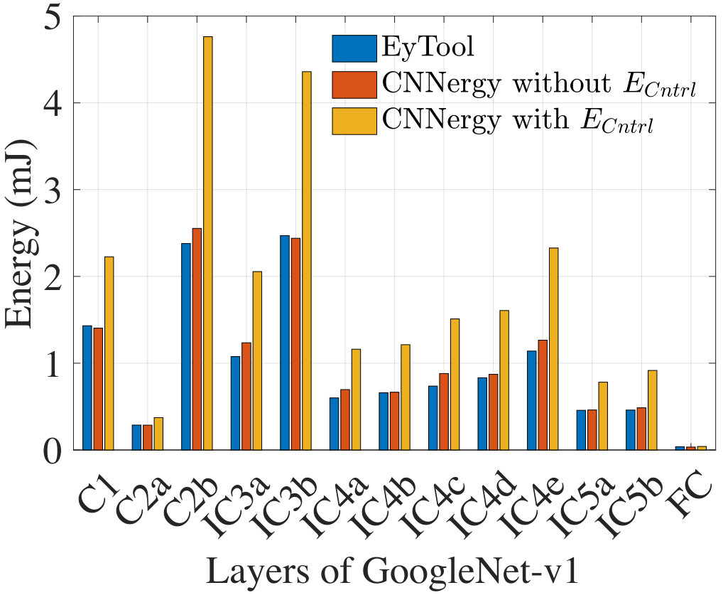 Figure 2
 Figure 3
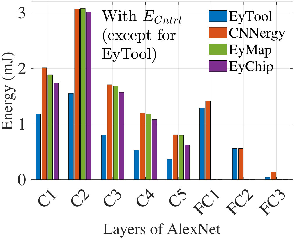 Figure 4
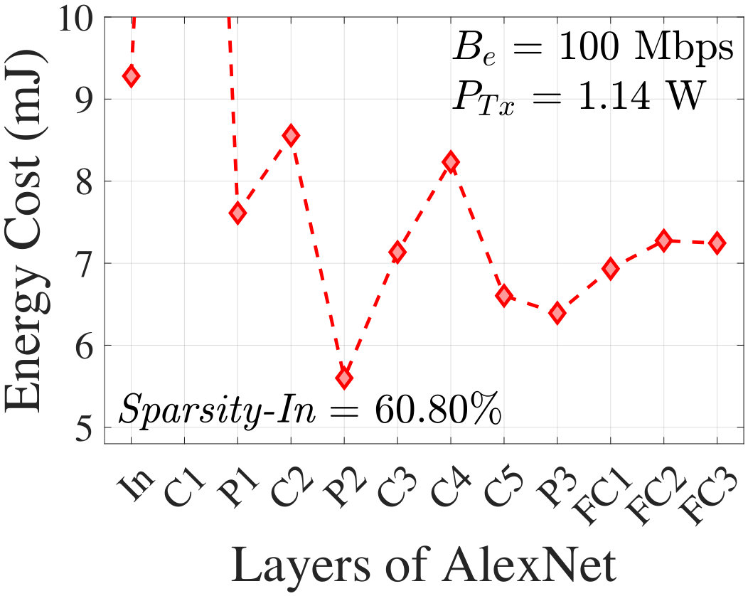 Figure 5
 Figure 6
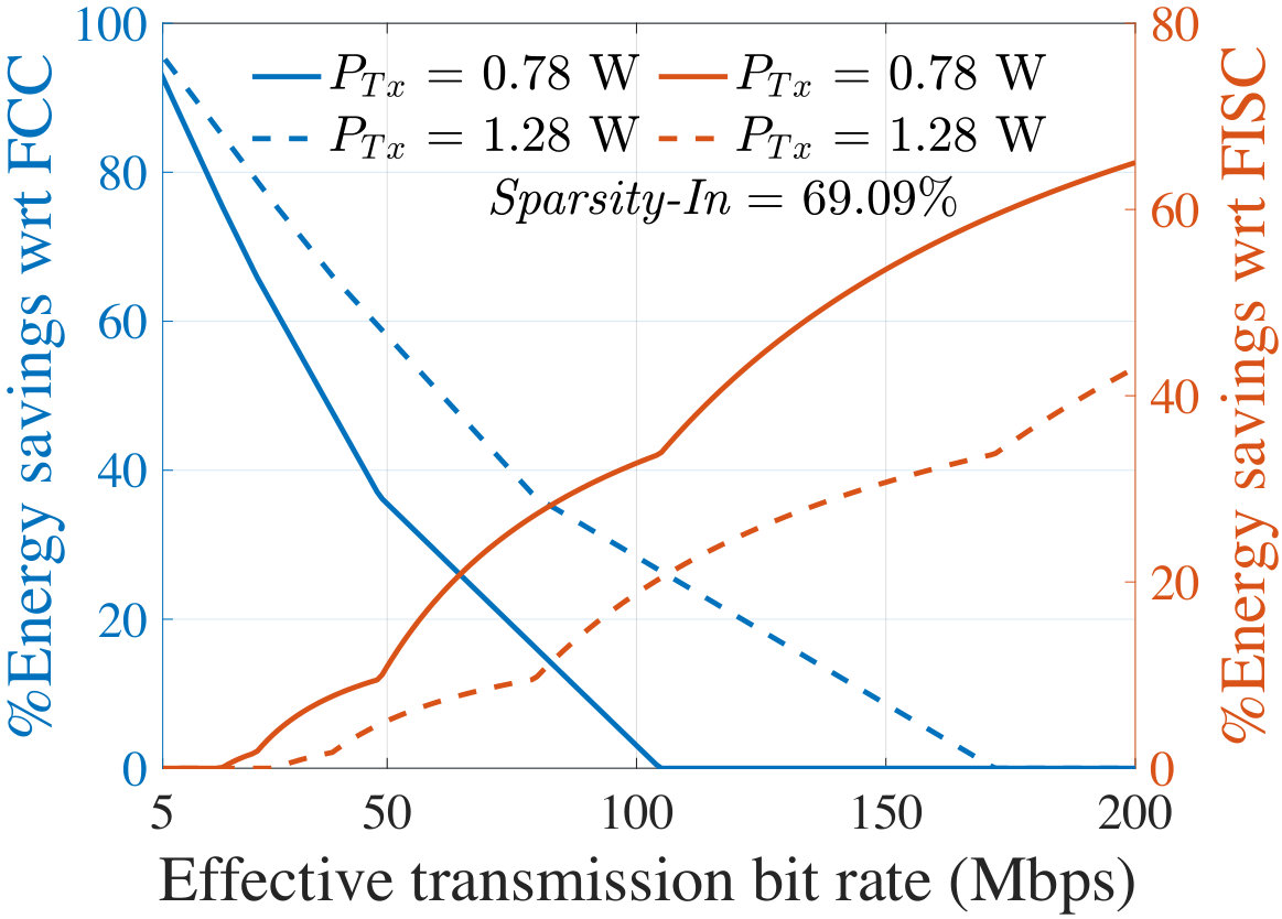 Figure 7
 Figure 8
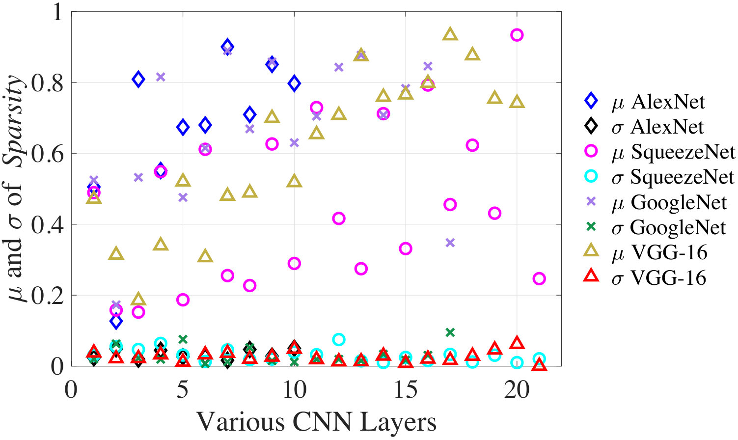 Figure 9
 Figure 10
 Figure 11
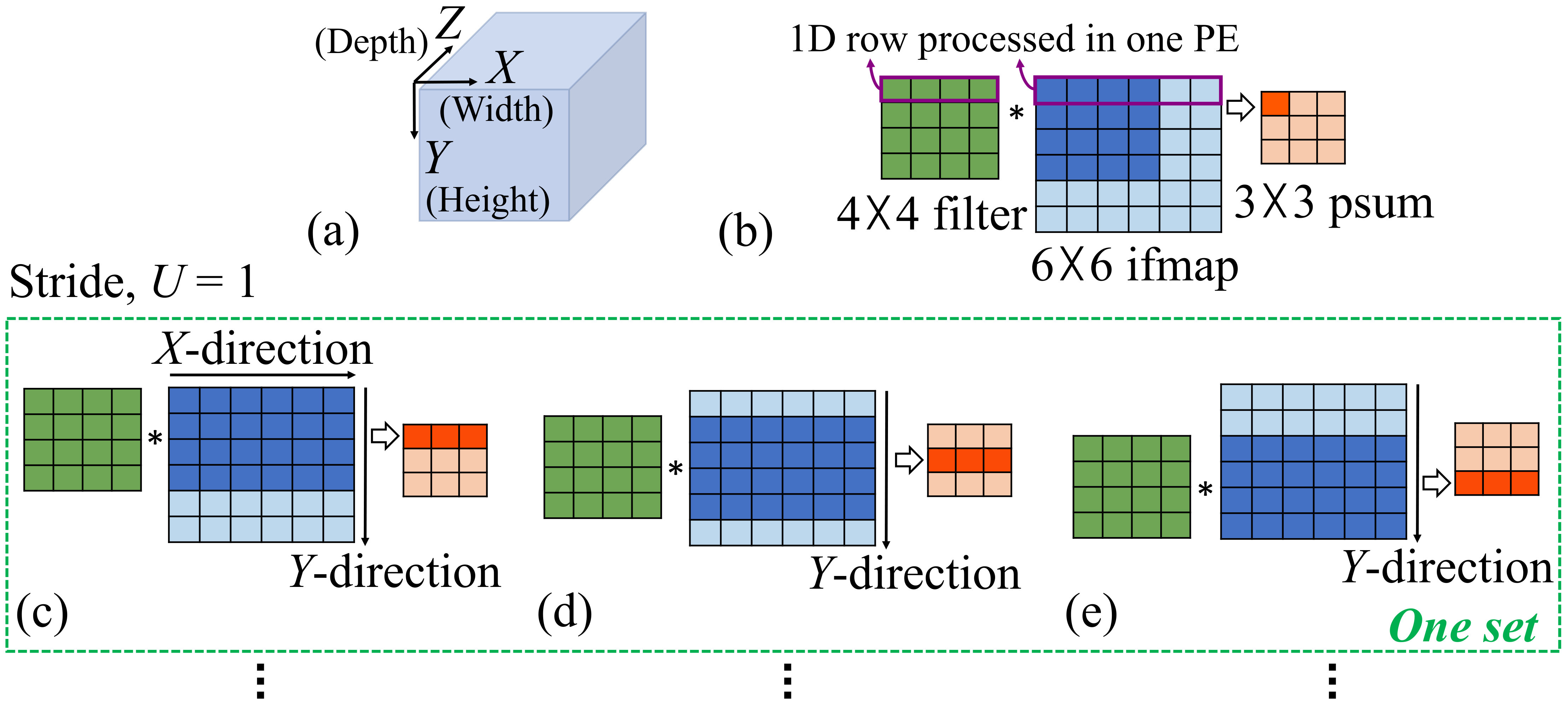 Figure 12
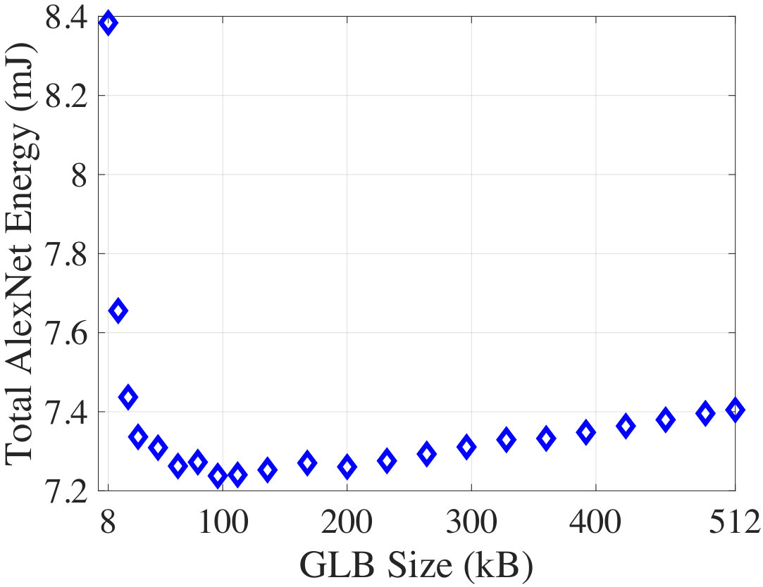 Figure 13
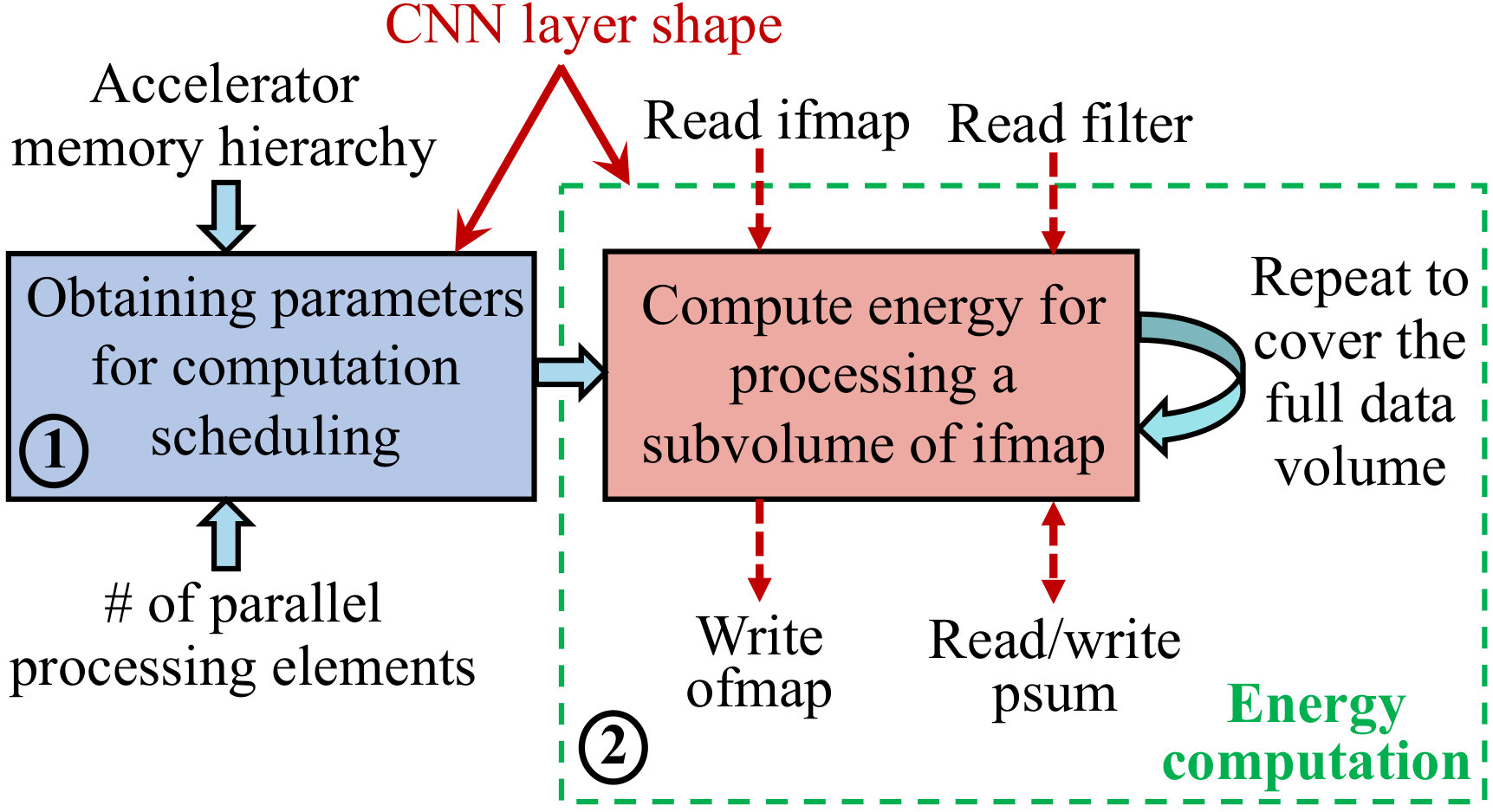 Figure 14
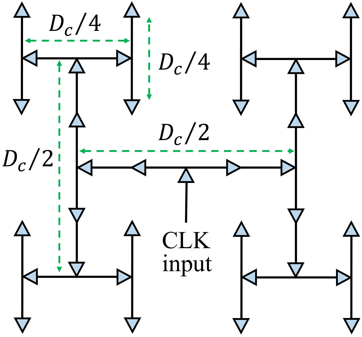 Figure 15
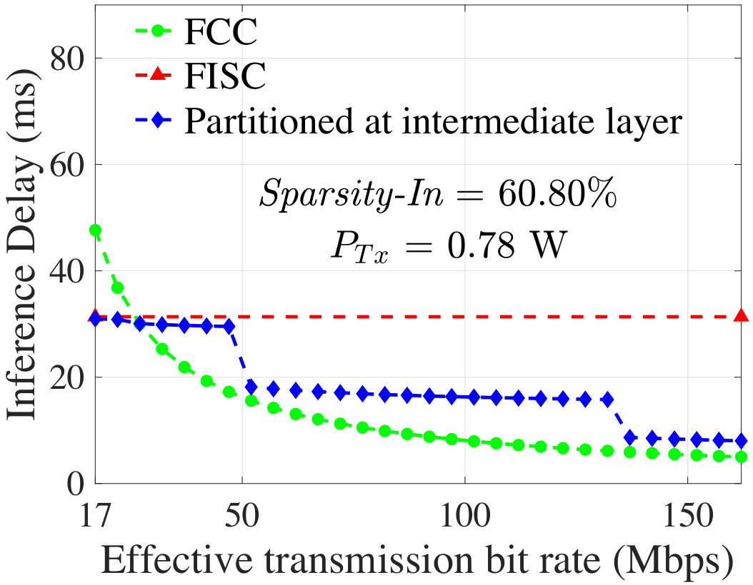 Figure 16
 Figure 17
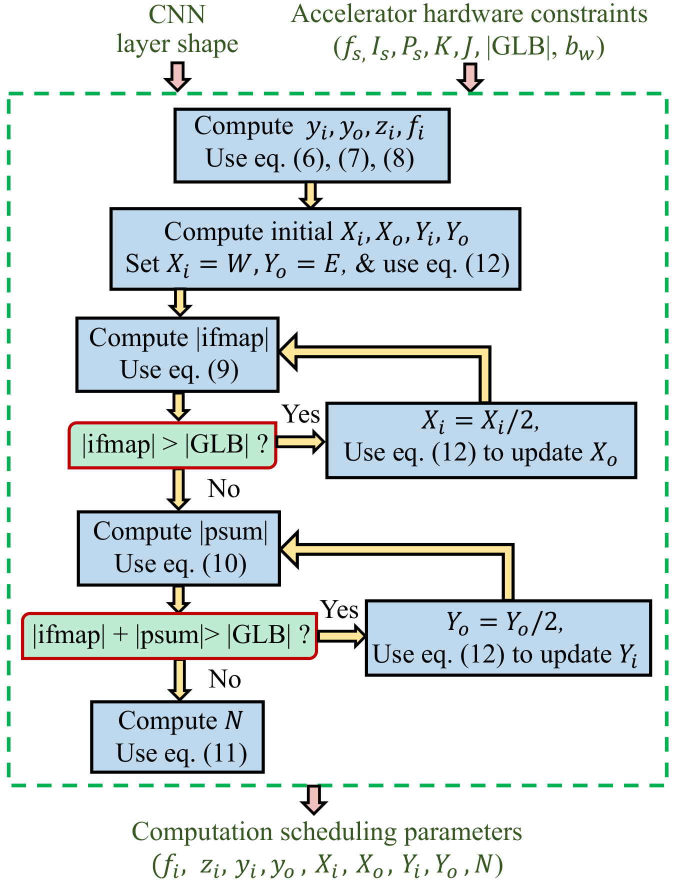 Figure 18
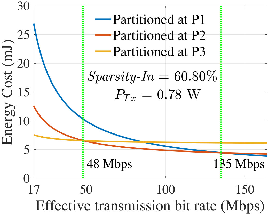 Figure 19
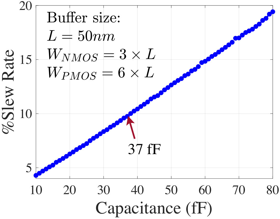 Figure 20
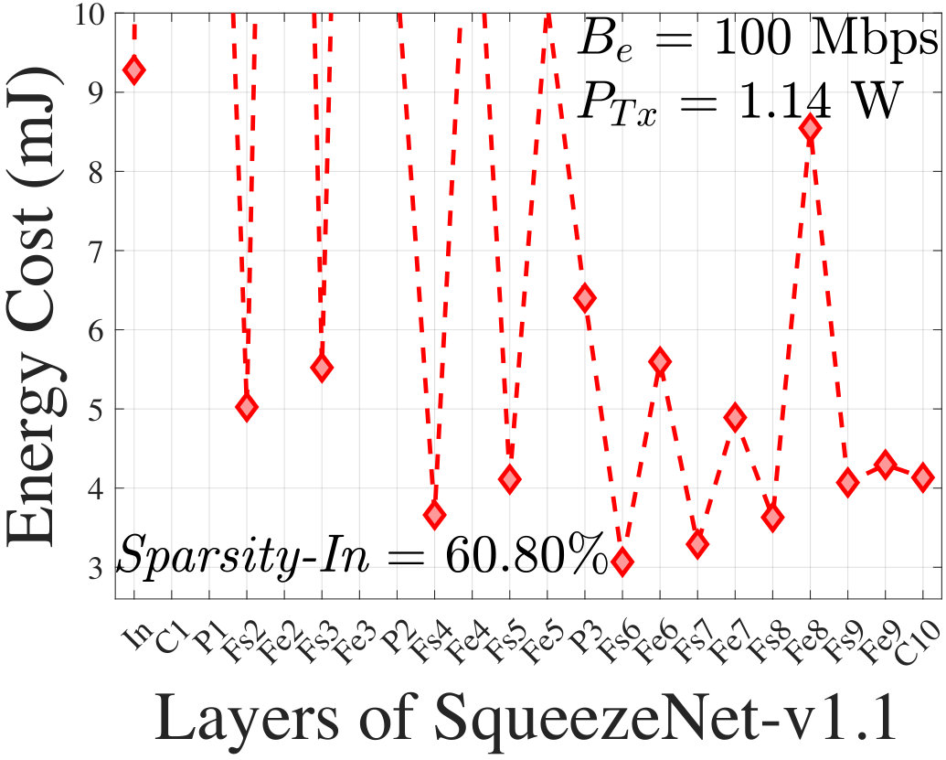 Figure 21
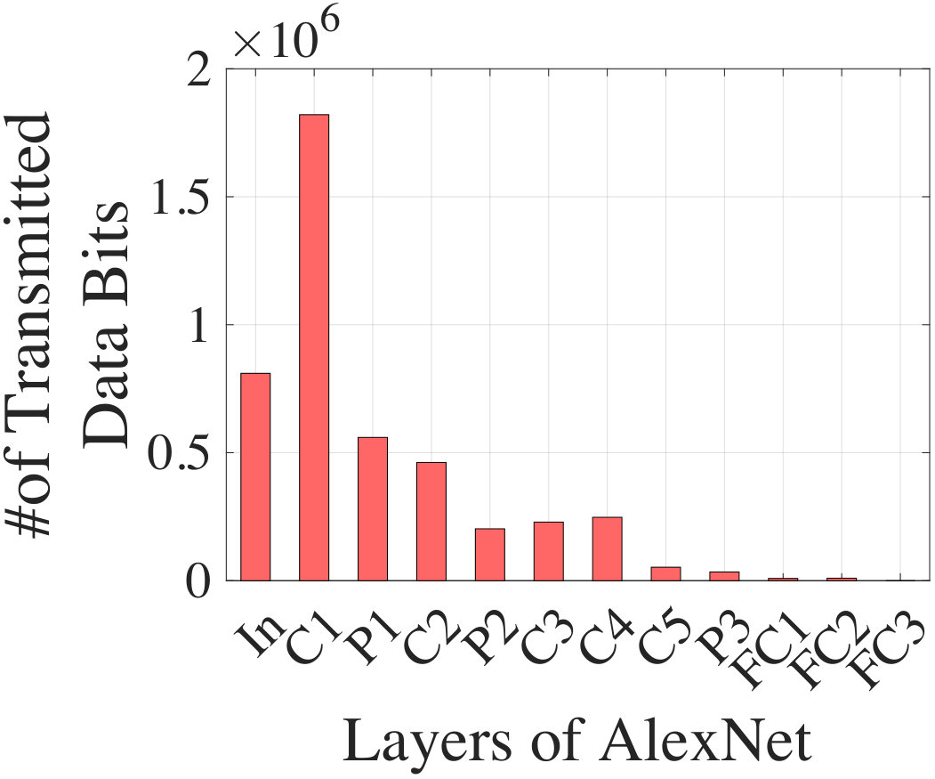 Figure 22
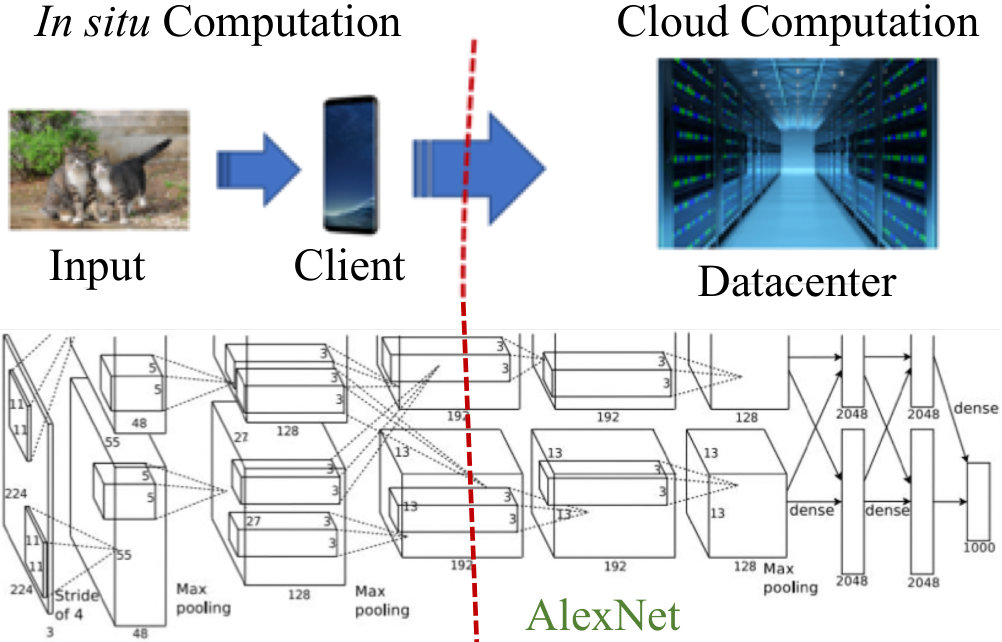 Figure 23
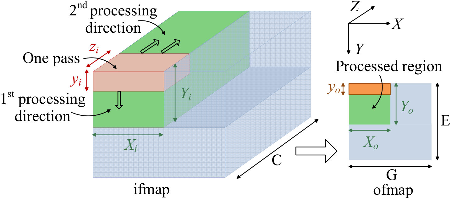 Figure 3
 Figure 25
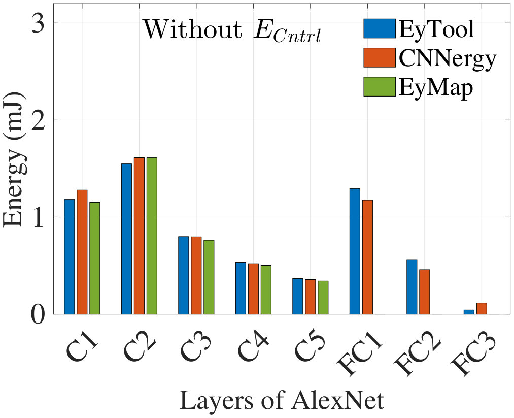 Figure 26
 Figure 27
 Figure 28
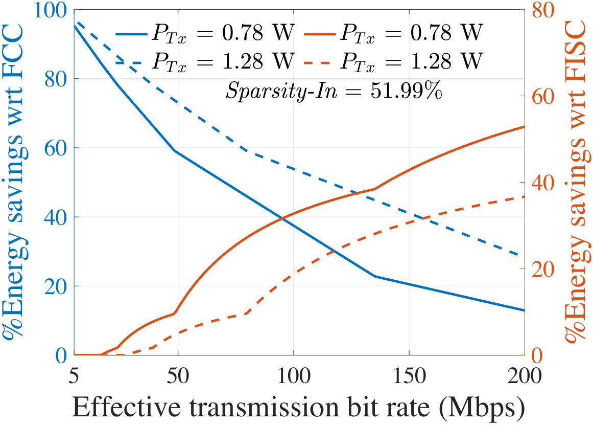 Figure 29
 Figure 30
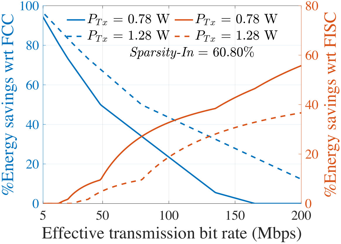 Figure 31
 Figure 32
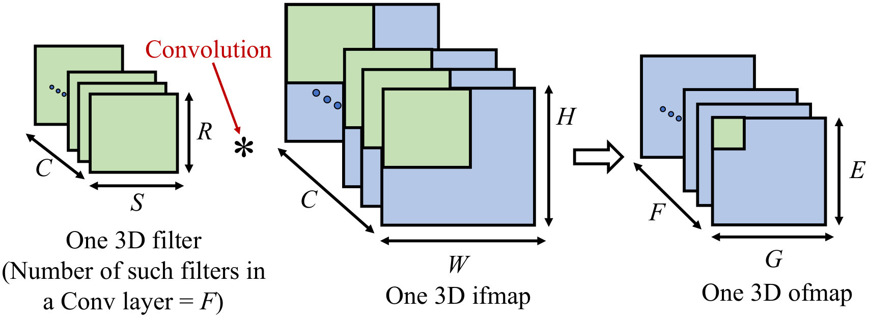 Figure 33
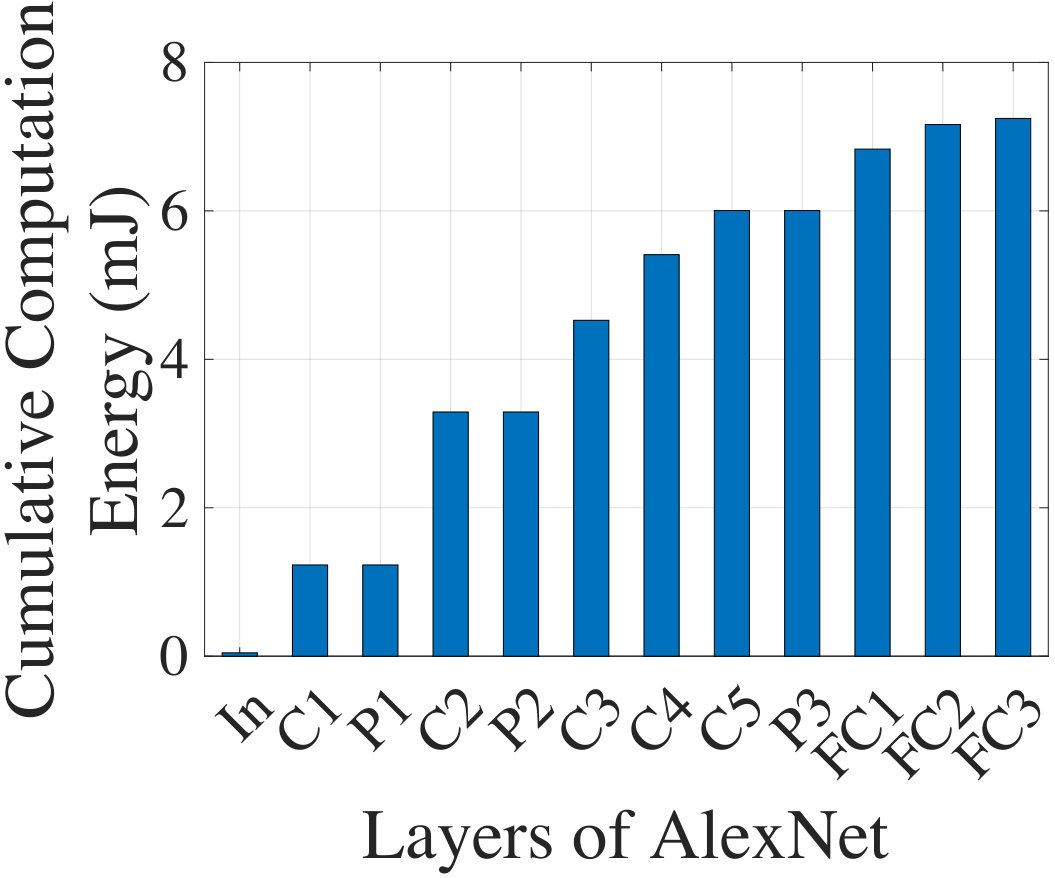 Figure 34
 Figure 35
 Figure 36
 Figure 37
 Figure 38
 Figure 39
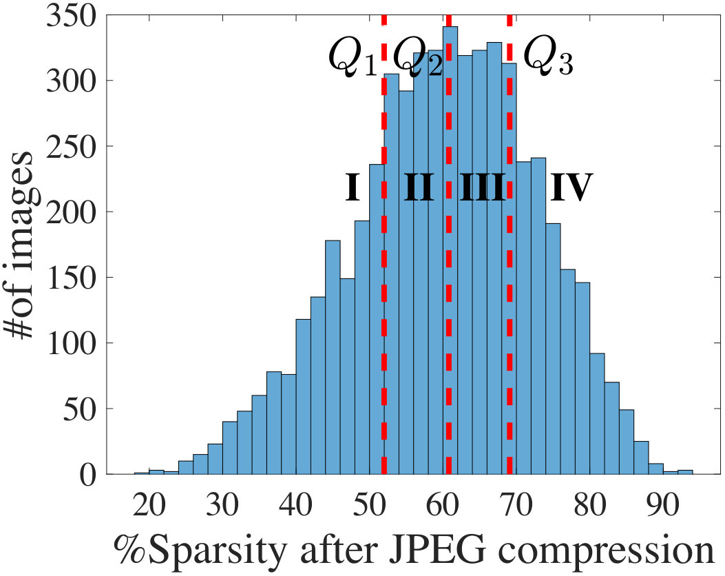 Figure 40
| Parameters | Description | ||
|---|---|---|---|
| Height/width of a filter | |||
| Padded height/width of an ifmap | |||
| Height/width of an ofmap | |||
| #of channels in an ifmap and filter | |||
|
|||
| Convolution stride |
| Notation | Description | ||
|---|---|---|---|
| Computation Scheduling Parameters | |||
| #of filters processed in a pass | |||
| #of ifmap/filter channels processed in a pass | |||
| () | Height of ifmap (ofmap) processed in a pass | ||
| () | Width of ifmap (ofmap) processed in a pass | ||
| () |
|
||
| #of ifmap from different images processed together | |||
| Accelerator Hardware Parameters | |||
| Size of RF storage for filter in one PE | |||
| Size of RF storage for ifmap in one PE | |||
| Size of RF storage for psum in one PE | |||
| Height of the PE array (#of rows) | |||
| Width of the PE array (#of columns) | |||
| GLB | Size of GLB storage | ||
| bit width of each data element | |||
| Average percent energy savings with respect to | |||||
| FCC | FISC | ||||
| CNN | Quartile | ||||
| I | II | III | IV | ||
| AlexNet | 52.4% | 40.1% | 25.7% | 4.1% | 27.3% |
| SqueezeNet | 73.4% | 66.5% | 58.4% | 38.4% | 28.8% |
| GoogleNet | 21.4% | 3.5% | 0.0% | 0.0% | 10.6% |
Peer Reviews
No public reviews on file for this paper yet. If you reviewed it on a platform where reviews are public (OpenReview, ICLR, NeurIPS, ICML), you can paste yours below so the community can read it here.
Code & Models
Videos
No videos yet. Explain this paper in a talk, walkthrough, or lecture? Add one.
NeuPart: Using Analytical Models to Drive Energy-Efficient Partitioning of CNN Computations on Cloud-Connected Mobile Clients
Susmita Dey Manasi, Farhana Sharmin Snigdha, and Sachin S. Sapatnekar Accepted April 28, 2020 for publication in IEEE Transactions on Very Large Scale Integration (VLSI) Systems. This work was supported in part by the National Science Foundation (NSF) under Award CCF-1763761. (Corresponding author: Susmita Dey Manasi.)The authors are with the Department of Electrical and Computer Engineering, University of Minnesota Twin Cities, Minneapolis, MN 55455 USA (e-mail: [email protected]; [email protected]; [email protected]).Digital Object Identifier 10.1109/TVLSI.2020.2995135
Abstract
Data processing on convolutional neural networks (CNNs) places a heavy burden on energy-constrained mobile platforms. This work optimizes energy on a mobile client by partitioning CNN computations between in situ processing on the client and offloaded computations in the cloud. A new analytical CNN energy model is formulated, capturing all major components of the in situ computation, for ASIC-based deep learning accelerators. The model is benchmarked against measured silicon data. The analytical framework is used to determine the optimal energy partition point between the client and the cloud at runtime. On standard CNN topologies, partitioned computation is demonstrated to provide significant energy savings on the client over fully cloud-based or fully in situ computation. For example, at 80 Mbps effective bit rate and 0.78 W transmission power, the optimal partition for AlexNet [SqueezeNet] saves up to 52.4% [73.4%] energy over a fully cloud-based computation, and 27.3% [28.8%] energy over a fully in situ computation.
Index Terms:
Embedded deep learning, Energy modeling, Hardware acceleration, Convolutional neural networks, Computation partitioning.
††publicationid: pubid:
© 2020 IEEE. Personal use of this material is permitted. Permission from IEEE must be obtained for all other uses, in any current or future media, including reprinting/republishing this material for advertising or promotional purposes, creating new collective works, for resale or redistribution to servers or lists, or reuse of any copyrighted component of this work in other works.
I Introduction
I-A Motivation
Machine learning using deep convolutional neural networks (CNNs) constitutes a powerful approach that is capable of processing a wide range of visual processing tasks with high accuracy. Due to the highly energy-intensive nature of CNN computations, today’s deep learning (DL) engines using CNNs are largely based in the cloud [1, 2], where energy is less of an issue than on battery-constrained mobile clients. Although a few simple emerging applications such as facial recognition are performed in situ on mobile processors, today’s dominant mode is to offload DL computations from the mobile device to the cloud. The deployment of specialized hardware accelerators for embedded DL to enable energy efficient execution of CNN tasks is the next frontier.
Limited client battery life places stringent energy limitations on embedded DL systems. This work focuses on a large class of inference engine applications where battery life considerations are paramount over performance: e.g., for a health worker in a remote area, who uses a mobile client to capture images processed using DL to diagnose cancer [3], a farmer who takes crop photographs and uses DL to diagnose plant diseases [4], or an unmanned aerial vehicle utilizing DL for monitoring populations of wild birds [5]. In all these examples, client energy is paramount for the operator in the field and processing time is secondary, i.e., while arbitrarily long processing times are unacceptable, somewhat slower processing times are acceptable for these applications. Moreover, for client-focused design, it is reasonable to assume that the datacenter has plentiful power supply, and the focus is on minimizing client energy rather than cloud energy. While this paradigm may not apply to all DL applications (e.g., our solution is not intended to be applied to applications such as autonomous vehicles, where high-speed data processing is important), the class of energy-critical client-side applications without stringent latency requirements encompasses a large corpus of embedded DL tasks that require energy optimization at the client end.
To optimize client energy, this work employs computation partitioning between the client and the cloud. Fig. 1 shows an inference engine computation on AlexNet [6], a representative CNN topology, for recognition of an image from the camera of a mobile client. If the CNN computation is fully offloaded to the cloud, the image from the camera is sent to the datacenter, incurring a communication overhead corresponding to the number of data bits in the compressed image. Fully in situ CNN computation on the mobile client involves no communication, but drains its battery during the energy-intensive computation.
Computation partitioning between the client and the cloud represents a middle ground: the computation is partially processed in situ, up to a specific CNN layer, on the client. The data is then transferred to the cloud to complete the computation, after which the inference results are sent back to the client, as necessary. We propose NeuPart, a partitioner for DL tasks that minimizes client energy. NeuPart is based on an analytical modeling framework, and analytically identifies, at runtime, the energy-optimal partition point at which the partial computation on the client is sent to the cloud.
Fig. 2 concretely illustrates the tradeoff between communication and computation for AlexNet. In (a), we show the cumulative computation energy (obtained from our analytical CNN energy model presented in Section IV) from the input to a specific layer of the network. In (b), we show the volume of compressed data that must be transmitted when the partial in situ computation is transmitted to the cloud. The data computed in internal layers of the CNN tend to have significant sparsity (over 80%, as documented later in Fig. 10): NeuPart leverages this sparsity to transmit only nonzero data at the point of partition, thus limiting the communication cost.
The net energy cost for the client for a partition at the layer can be computed as:
[TABLE]
where is the processing energy on the client, up to the CNN layer, and is the energy required to transmit this partially computed data from the client to the cloud. The inference result corresponds to a trivial amount of data to return the identified class, and involves negligible energy.
NeuPart focuses on minimizing for the energy-constrained client. For the data in Fig. 2, increases monotonically as we move deeper into the network, but can reduce greatly. Thus, the optimal partitioning point for here lies at an intermediate layer .
I-B Contributions of NeuPart
The specific contributions of NeuPart are twofold:
- •
We develop a new analytical energy model (we name our model “CNNergy” which is the core of NeuPart) to estimate the energy of executing CNN workload (i.e., ) on an ASIC-based deep learning (DL) accelerator.
- •
Unlike prior computation partitioning works [7, 8, 9, 10, 11, 12], NeuPart addresses the client/cloud partitioning problem for specialized DL accelerators that are more energy-efficient than CPU/GPU/FPGA-based platforms.
Today, neural networks are driving research in many fields and customized neural hardware is possibly the most active area in IC design research. While there exist many simulation platforms for performance analysis for general-purpose processors [13], memory systems [14], and NoCs [15], there is no comparable performance simulator for ASIC implementations of CNNs. Our model, CNNergy, is an attempt to fill that gap. CNNergy accounts for the complexities of scheduling computations over multidimensional data. It captures key parameters of the hardware and maps the hardware to perform computation on various CNN topologies. CNNergy is benchmarked on several CNNs: AlexNet, SqueezeNet-v1.1 [16], VGG-16 [17], and GoogleNet-v1 [18]. CNNergy is far more detailed than prior energy models [19] and incorporates implementation specific details of a DL accelerator, capturing all major components of the in situ computation, including the cost of arithmetic computations, memory and register access, control, and clocking. It is important to note that, for an ASIC-based neural accelerator platform, unlike a general-purpose processor, the computations are highly structured and the memory fetches are very predictable. Unlike CPUs, there are no conditionals or speculative fetches that can alter program flow significantly. Therefore, an analytical modeling framework (as validated in Section V) is able to predict the CNN energy consumption closely for the custom ASIC platform.
CNNergy may potentially have utility beyond this work, and has been open-sourced at https://github.com/manasiumn37/CNNergy. For example, it provides a breakdown of the total energy into specific components, such as data access energy from different memory levels of a DL accelerator, data access energy associated with each CNN data type from each level of memory, MAC computation energy. CNNergy can also be used to explore design phase tradeoffs such as analyzing the impact of changing on-chip memory size on the total execution energy of a CNN. We believe that our developed simulator (CNNergy) will be useful to the practitioners who need an energy model for CNNs to evaluate various design choices. The application of data partitioning between client and cloud shows a way to apply our energy model to a practical scenario.
The paper is organized as follows. Section II discusses prior approaches to computational partitioning and highlights the differences of NeuPart as compared to the prior works. In Section III, fundamental background on CNN computation is provided, and the general framework of CNNergy for CNN energy estimation on custom ASIC-based DL accelerators is outlined. Next, Sections IV presents the detailed modeling of CNNergy and is followed by Section V, which validates the model in several ways, including against silicon data. Section VI presents the models for the estimation of transmission energy as well as inference delay. A method for performing the NeuPart client/cloud partitioning at runtime is discussed in Section VII. Finally, in Section VIII, the evaluations of the client/cloud partitioning using NeuPart is presented under various communication environments for widely used CNN topologies. The paper concludes in Section IX.
II Related Work
Computational partitioning has previously been used in the general context of distributed processing [20]. A few prior works [7, 8, 9, 10, 11, 12] have utilized computation partitioning in the context of mobile DL. In [7], tasks are offloaded to a server from nearby IoT devices for best server utilization, but no attempt is made to minimize edge device energy. In [8] and [9], partitioning is used to optimize overall delay or throughput for delay critical applications of deep neural network (DNN) (e.g., self-driving cars [8]). Another work, [10], uses partitioning between the client and local server (in contrast to centralized cloud) where along with the inference data, the client also needs to upload the partial DNN model (i.e., DNN weights) to the local server every time it makes an inference request. Therefore, the optimization goals and the target platforms of these works are very different from NeuPart.
The work in [11] uses limited application-specific profiling data to schedule computation partitioning. Another profiling-based scheme [12] uses client-specific profiling data to form a regression-based computation partitioning model for each device. A limitation of profiling-based approaches is that they require profiling data for each mobile device or each DL application, which implies that a large number of profiling measurements are required for real life deployment. Moreover, profiling-based methods require the hardware to already be deployed and cannot support design-phase optimizations. Furthermore, all these prior approaches use a CPU/GPU-based platform for the execution of DL workloads.
In contrast with prior methods, NeuPart works with specialized DL accelerators, which are orders of magnitude more energy-efficient as compared to the general-purpose machines [1, 21, 22], for client/cloud partitioning. NeuPart specifically leverages the highly structured nature of computations on CNN accelerators, and shows that an analytical model predicts the client energy accurately (as demonstrated in Section V). The analytical framework used in the NeuPart CNNergy incorporates implementation-specific details that are not modeled in prior works. For example, the work in Neurosurgeon [12] uses (a) uncompressed raw image to transmit at the input, which is not typical: in a real system, images are compressed before transmission to reduce the communication overhead; (b) unequal bit width (i.e., 32-bit data for the intermediate layers while 8-bit data for the input layer; and (c) ignores any data sparsity at the intermediate CNN layers. Consequently, these cause the partitioning decision by Neurosurgeon to be either client-only or cloud-only in most cases. In contrast, in addition to using a specialized DL accelerator, NeuPart fully leverages the inherent computation-communication tradeoff of CNNs by exploiting their key properties and shows that (Fig. 13 in Section VIII) there is a wide space where an intermediate partitioning point can offer significant energy savings as compared to the client-only or cloud-only approaches.
III Computations on CNN Hardware
III-A Fundamentals of CNNs
The computational layers in CNNs can be categorized into three types: convolution (Conv), fully connected (FC), and pooling (Pool). The computation in a CNN is typically dominated by the Conv layers. In each layer, the computation involves three types of data:
- •
ifmap, the input feature map
- •
filter, the filter weights, and
- •
psum, the intermediate partial sums.
Table I summarizes the parameters associated with a convolution layer. As shown in Fig. 3, for a Conv layer, filter and ifmap are both 3D data types consisting of multiple 2D planes (channels). Both the ifmap and filter have the same number of channels, , while and .
During the convolution, an element-wise multiplication between the filter and the green 3D region of the ifmap in Fig. 3 is followed by the accumulation of all products (i.e., psums), and results in one element shown by the green box in the output feature map (ofmap). Each channel () of the filter slides through its corresponding channel () of the ifmap with a stride (), repeating similar multiply-accumulate (MAC) operations to produce a full 2D plane () of the ofmap. A nonlinear activation function (e.g., a rectified linear unit, ReLU) is applied after each layer, introducing sparsity (i.e., zeros) at the intermediate layers, which can be leveraged to reduce computation.
The above operation is repeated for all filters to produce 2D planes for the ofmap, i.e., the number of channels in the ofmap equals the number of 3D filters in that layer. Due to the nature of the convolution operation, there is ample opportunity for data reuse in a Conv layer. FC layers are similar to Conv layers but are smaller in size, and produce a 1D ofmap. Computations in the Pool layers serve to reduce dimensionality of the ofmaps produced from the Conv layers by storing the maximum/average value over a window of the ofmap.
III-B Executing CNN Computations on a Custom ASIC
III-B1 Architectural Features of CNN Hardware Accelerators
Since the inference task of a CNN comprises a very structured and fixed set of computations (i.e., MAC, nonlinear activation, pooling, and data access for the MAC operands), specialized hardware accelerators are very suitable for their execution. Various dedicated accelerators have been proposed in the literature for the efficient processing of CNNs [1, 23, 24, 22, 25, 26]. The architecture in Google TPU [1] consists of a 2D array of parallel MAC computation units, a large on-chip buffer for the storage of ifmap and psum data, additional local storage inside the MAC computation core for the filter data, and finally, off-chip memory to store all the feature maps and filters together. Similarly, along with an array of parallel processing elements, the architectures in [26, 24, 22, 25] use a separate on-chip SRAM to store a chuck of filter, ifmap, and psum data, and an external DRAM to completely store all the ifmap/ofmap and filter data. In [22, 23], local storage is used inside each processing element while allowing data communication between processing elements to facilitate better reuse of data. Additionally, [26, 25, 23] exploit the inherent data sparsity in the internal layers of CNN to save computation energy.
It is evident that the key architectural features of these accelerators are fundamentally similar: an array of processing elements to perform neural computation in parallel, multiple levels of memory for fast data access, and greater data reuse. We utilize these key architectural features of ASIC hardware to develop the general framework of CNNergy.
III-B2 General Framework of CNNergy
We develop CNNergy to estimate the energy dissipation in a CNN hardware accelerator. The general framework of CNNergy is illustrated in Fig. 4. We use CNNergy to determine the in situ computation energy ( in (1)), accounting for scheduling and computation overheads.
One of the largest contributors to energy is the cost of data access from memory. Thus, data reuse is critical for energy-efficient execution of CNN computations to reduce unnecessary high-energy memory accesses, particularly the ifmap and filter weights, and is used in [1, 23, 22, 25, 26]. This may involve, for example, ifmap and filter weight reuse across convolution windows; ifmap reuse across filters, and reduction of psum terms across channels. Given the accelerator memory hierarchy, number of parallel processing elements, and CNN layer shape, Block 1 of Fig. 4 is an automated scheme for scheduling MAC computations while maximizing data reuse. The detailed methodology for obtaining these scheduling parameters is presented in Section IV-C.
Depending on the scheduling parameters, the subvolume of the ifmap to be processed at a time is determined. Block 2 then computes the corresponding energy for the MAC operations and associated data accesses. The computation in Block 2 is repeated to process the entire data volume in a layer, as detailed in Section IV-D.
The framework of CNNergy is general and its principles apply to a large class of CNN accelerators. However, to validate the framework, we demonstrate it on a specific platform, Eyeriss [23], for which ample performance data is available, including silicon measurements. Eyeriss has an array of processing elements (PEs), each with:
- •
a multiply-accumulate (MAC) computation unit.
- •
register files (RFs) for filter, ifmap, and psum data.
We define , , and as the maximum number of -bit filter, ifmap, and psum elements that can be stored in a PE.
The accelerator consists of four levels of memory: DRAM, global SRAM buffer (GLB), inter-PE RF access, and local RF within a PE. During the computations of a layer, filters are loaded from DRAM to the RF. In the GLB, storage is allocated for psum and ifmap. After loading data from DRAM, ifmaps are stored into the GLB to be reused from the RF level. The irreducible psums navigate through GLB and RF as needed. After complete processing of a 3D ifmap, the ofmaps are written back to DRAM.
IV Analytical CNN Energy Model
We formulate an analytical model (CNNergy) for the CNN processing energy (used in (1)), , up to the layer, as
[TABLE]
where is the energy required to process layer of the CNN. To keep the notation compact, we drop the index “” in the remainder of this section. We can write as:
[TABLE]
where is the energy to compute MAC operations associated with the layer, represents the energy associated with the control and clocking circuitry in the accelerator, and is the memory data access energy,
[TABLE]
i.e., the sum of data access energy from on-chip memory (from GLB, Inter-PE, and RF), and from the off-chip DRAM.
The computation of these energy components, particularly the data access energy, is complicated by their dependence on the data reuse pattern in the CNN. In Sections IV-A to IV-D, we develop a heuristic for optimal data reuse and describe the methodology in our CNNergy for estimating these energy components.
Specifically, in Section IV-A, we conceptually demonstrate how CNNergy processes the 3D data volume by dividing it into multiple subvolumes. We also define the parameters to schedule the CNN computation in this section. Next, in Section IV-B, we describe the dataflow to distribute the convolution operation in the PE array and identify the degrees of freedom to map the computation in the hardware. In Section IV-C, we present our automated mapping scheme to compute the computation scheduling parameters for any given CNN layer. Finally, using the scheduling parameters, we present the steps to compute energy for each component of (3) in Section IV-D.
IV-A Conceptual Illustration of CNNergy
Fig. 5 illustrates how the 3D ifmap is processed by convolving one 3D filter with ifmap to obtain one 2D channel of ofmap; this is repeated over all filters to obtain all channels of ofmap. Due to the large volume of data in a CNN layer and the limited availability of on-chip storage (register files and SRAM), the data is divided into smaller subvolumes, each of which is processed by the PE array in one pass** to generate psums, where the capacity of the PE array and local storage determine the amount of data that can be processed in a pass.**
All psums are accumulated to produce the final ofmap entry; if only a subset of psums are accumultated, then the generated psums are said to be irreducible. The pink region of size shows the ifmap volume that is covered in one pass, while the green region shows the volume that is covered in multiple passes before a write-back to DRAM.
As shown in the figure (for reasons provided in Section IV-C), consecutive passes first process the ifmap in the -direction, and then the -direction, and finally, the -direction. After a pass, irreducible psums are written back to GLB, to be later consolidated with the remainder of the computation to build ofmap entries. After processing the full -direction (i.e., all the channels of a filter and ifmap) the green ofmap region of size is formed and then written back to DRAM. The same process is then repeated until the full volume of ifmap/ofmap is covered.
Fig. 5 is a simplified illustration that shows the processing of one 3D ifmap using one 3D filter. Depending on the amount of available register file storage in the PE array, a convolution operation using filters can be performed in a pass. Furthermore, subvolumes from multiple images (i.e., ifmaps) can be processed together, depending on the SRAM storage capacity.
Due to the high cost of data fetches, it is important to optimize the pattern of fetch operations from the DRAM, GLB, and register file by reusing the fetched data. The level of reuse is determined by the parameters , , , , , , , , and . Hence, the efficiency of the computation is based on the choice of these parameters. The mapping approach that determines these parameters, in a way that attempts to minimize data movement, is described in Section IV-C.
IV-B Dataflow Illustration in the PE array
In this section we describe how the convolution operations are distributed in the 2D PE array of size . We use the row-stationary scheme to manage the dataflow for convolution operations in the PE array as it is shown to offer higher energy-efficiency than other alternatives ****[27, 28]****.
IV-B1 Processing the ifmap in Sets – Concept
We explain the row-stationary dataflow with a simplified example shown in Fig. 6, where a single channel of the filter and ifmap are processed (i.e., ). Fig. 6(b) shows a basic computation where a filter (green region) is multiplied with the part of the ifmap that it is overlaid on, shown by the dark blue region. Based on the row-stationary scheme for the distributed computation, these four rows of the ifmap are processed in four successive PEs within a column of the PE array. Each PE performs an element-wise multiplication of the ifmap row and the filter row to create a psum. The four psums generated are transmitted to the uppermost PEs and accumulated to generate their psum (dark orange).
Extending this operation to a full convolution implies that the ifmap slides under the filter in the negative -direction with a stride of , while keeping the filter stationary: for , two strides are required to cover the ifmap in the -direction. In our example, for each stride, each of the four PEs performs the element-wise multiplication between one filter row and one ifmap row, producing one 1D row of psum, which is then accumulated to produce the first row of psum, as illustrated in Fig. 6(c).
Thus, the four dark blue rows in Fig. 6(c) are processed by four PEs (one per row) in a column of the PE array. The reuse of the filter avoids memory overheads due to repeated fetches from other levels of memory. To compute psums associated with other rows of the ofmap, a subarray of 12 PEs (4 rows 3 columns) processes the ifmap under a -direction ifmap stride. The ifmap regions thus processed are shown by the dark regions of Fig. 6(d),(e).
We define the amount of processing performed in rows, across all columns of the PE array, as a set. For a PE array, a set coresponds to the processing in Fig. 6(c)–(e).
In the general context of the PE array, a set is formed from PEs. Therefore, the number of sets which can fit in the full PE array (i.e., the number of sets in a pass) is given by:
[TABLE]
i.e., is the ratio of the PE array height to the filter height.
IV-B2 Processing the ifmap in Sets – Realistic Scenario
We now generalize the previously simplified assumptions in the example to consider typical parameter ranges. We also move from the assumption of , to a more typical .
First, the filter height can often be less than the size of the PE array. When , the remaining PE array rows can process more filter channels simultaneously, in multiple sets.
Second, typical RF sizes in each PE are large enough to operate on more than one 1D row. Under this scenario, within each set, a group of 2D filter planes is processed. There are several degrees of freedom in mapping computations to the PE array. When several 1D rows are processed in a PE, the alternatives for choosing this group of 1D rows include:
- (i)
choosing filter/ifmap rows from different channels of the same 3D filter/ifmap; 2. (ii)
choosing filter rows from different 3D filters; 3. (iii)
combining (i) and (ii), where some rows come from the channels of the same 3D filter and some rows come from the channels under different 3D filters.
Across sets** in the PE array, similar mapping choices are available. Different groups of filter planes (i.e., channels) are processed in different sets. These groups of planes can be chosen either from the same 3D filter, or from different 3D filters, or from a combination of both.**
Thus, there is a wide space of mapping choices for performing the CNN computation in the PE array.
IV-B3 Data Reuse
Due to the high cost of data accesses from the next memory level, it is critical to reuse data as often as possible to achieve energy efficiency. Specifically, after fetching data from a higher access-cost memory level, data reuse refers to the use of that data element in multiple MAC operations. For example, after fetching a data element from GLB to RF, if that data is used across MAC operations, then the data is reused times with respect to the GLB level.
We now examine the data reuse pattern within the PE array. Within each PE column, an ifmap plane is being processed along the -direction, and multiple PE columns process the ifmap plane along the -direction. Two instances of data reuse in the PE array are:
- (1)
In each set, the same ifmap row is processed along the PEs in a diagonal of the set. This can be seen in the example set in Fig. 6(c)-(e), where the third row of the ifmap plane is common in the PEs in in (c), in (d), and in (e), where refers to the PE in row and column . 2. (2)
The same filter row is processed in the PEs in a row: in Fig. 6(c)-(e), the first row of the filter plane is common to all PEs in all three columns of row 1.
Thus, data reuse can be enabled by broadcasting the same ifmap data (for instance (1)) and the same filter data (for instance (2)) to multiple PEs for MAC operations after they are fetched from a higher memory level (e.g., DRAM or GLB).
IV-C Obtaining Computation Scheduling Parameters
As seen in Section IV-B, depending on the specific CNN and its layer structure, there is a wide space of choices for computations to be mapped to the PE array. The mapping of filter and ifmap parameters to the PE array varies with the CNN and with each layer of a CNN. This mapping is a critical issue in ensuring low energy, and therefore, in this work, we develop an automated mapping scheme for any CNN topology. The scheme computes the parameters for scheduling computations. The parameters are described in Section IV-A and summarized in Table II. The table also includes the parameters for the accelerator hardware constraints.
For general CNNs, for each layer, we develop a mapping strategy that follows predefined rules to determine the computation scheduling. The goal of scheduling is to attempt to minimize the movement of three types of data (i.e., ifmap, psum, and filter), since data movement incurs large energy overheads. In each pass, the mapping strategy uses the following priority rules:
(i)** We process the maximum possible channels of an ifmap to reduce the number of psum terms that must move back and forth with the next level of memory.**
(ii)** We prioritize filter reuse, psum reduction over ifmap reuse.**
The rationale for Rules (i) and (ii) is that since a very large number of psums are generated in each layer, psum reduction is the most important factor for energy, particularly because transferring psums to the next pass involves expensive transactions with the next level of memory. This in turn implies that filter weights must remain stationary for maximal filter reuse. Criterion (ii) lowers the number of irreducible psums: if the filter is changed and ifmap is kept fixed, the generated psums are not reducible.
In processing the ifmap, proceeding along the - and -directions enables the possibility of filter reuse as the filter is kept stationary in the RF while the ifmap is moved. In contrast, if passes were to proceed along the -direction, filter reuse would not be possible since new filter channels must be loaded from the DRAM for the convolution with ifmap. Therefore, the -direction is the last to be processed. In terms of filter reuse, the - and -directions are equivalent, and we arbitrarily prioritize the -direction over the -direction.
We use the notion of a set and a pass (Section IV-B) in the flow graph to devise the choice of scheduling parameters:
IV-C1 Computing and
The value of and is limited by the number of columns, , in the PE array. The corresponding value of is found using the relation
[TABLE]
IV-C2 Computing and
The number of channels of each ifmap in a pass is computed as
[TABLE]
where is the number of channels per set, and is the number of sets per pass (given by (5)). Recall that the first priority rule of CNNergy is to process the largest possible number of ifmap channels at a time. Therefore, to compute , we find the number of filter rows that can fit into an ifmap RF, i.e., .
To enable per-channel convolution, the filter RF of a PE must be loaded with the same number of channels as from a single filter. The remainder of the dedicated filter RF storage can be used to load channels from different filters so that one ifmap can be convolved with multiple filters resulting in ifmap reuse. Thus, after maximizing the number of channels of an ifmap/filter to be processed in a pass, the remaining storage can be used to enable ifmap reuse. Therefore, the number of filters processed in a pass is
[TABLE]
IV-C3 Computing , , , ,
During a pass, the ifmap corresponds to the pink region in Fig. 5, and over multiple passes, the entire green volume of the ifmap in the figure is processed before a writeback to DRAM.
We first compute ifmap and psum, the storage requirements of ifmap and psum, respectively, during the computation. The pink region has dimension and over several passes it creates, for each of the filters, a set of psums for the region of the ofmap that are not fully reduced (i.e., they await the results of more passes). Therefore,
[TABLE]
where corresponds to the bit width for ifmap and psum.
Next, we determine how many ifmap passes can be processed for a limited GLB size, GLB. This is the number, , of pink regions that can fit within the GLB, i.e.,
[TABLE]
To compute , we first set it to the full ifmap width, , and we set to the full ofmap height, , to obtain . If , i.e., ifmappsumGLB, then and are reduced until the data fits into the GLB and .
From the values of and computed above, we can determine and using the relations
[TABLE]
Fig. 7 shows the flow graph that summarizes how the parameters for scheduling the CNN computation are computed. The module takes the CNN layer shape (Table I) and the accelerator hardware parameters (Table II) as inputs. Based on our automated mapping strategy, the module outputs the computation scheduling parameters (Table II).
IV-C4 Exception Rules
The mapping method handles exceptions:
- •
If , some PE columns will remain unused. This is avoided by setting . If the new ifmappsumGLB, is reduced so that the data fits into the GLB.
- •
If , all channels are processed in a pass while increasing , as there is more room in the PE array to process more filters. The cases , proceed by reducing .
- •
All Conv layers whose filter has the dimension (e.g., inside the inception modules of GoogleNet, or the fire modules of SqueezeNet) are handled under a fixed exception rule that uses a reduced , and suitably increased .
The exceptions are triggered only for a few CNN layers (i.e., layers having relatively few channels or filters).
IV-D Energy () Computation
In Section IV-C, we have determined the subvolume of ifmap and filter data to be processed in a pass. From the scheduling parameters we can also compute the number of passes before a writeback of ofmap to DRAM. Therefore, we have determined the schedule of computations to generate all channels of ofmap. We now estimate each component of in (3). The steps for this energy computation are summarized in Algorithm 1, which takes as input the computation scheduling parameters, CNN layer shape parameters, and technology-dependent parameters that specify the energy per operation (Table III), and outputs .
IV-D1 Computing ,
We begin by computing the subvolume of data loaded in each pass (Lines 1–5). In Fig 5, is illustrated as the pink ifmap region which is processed in one pass for an image, and is the number of psum entries associated with the orange ofmap region for a single filter and single image. The filter data is reused across () passes, and we denote the number of filter elements loaded for these passes by . Thus, for filters and images,
[TABLE]
To compute energy, we first determine , the data access energy required to process volume of each ifmap over filters and images. In each pass, a volume of the ifmap is brought from the DRAM to the GLB for data access; psums move between GLB and RF; and RF-level data accesses () occur for the four operands associated with each MAC operation in a pass. Therefore, the corresponding energy can be computed as:
[TABLE]
Here, denotes the energy associated with operation , and each energy component can be computed by multiplying the energy per operation by the number of operations. Since filter data is reused across () passes, all components in (16), except the energy associated with filter access, are multiplied by this factor. Each psum is written once and read once, and accounts for both operations.
Next, all channels of ifmap (i.e., the entire green ifmap region in Fig. 5) are processed to form the green region of each ofmap channel, and this data is written back to DRAM. To this end, we compute , the data access energy to produce fraction of each ofmap channel over filters and images, by repeating the operations in (16) to cover all the channels:
[TABLE]
Finally, the computation in (17) is repeated to produce the entire volume of the ofmap over all filters. Therefore, the total energy for data access is
[TABLE]
Here, the multipliers , , and represent the number of iterations of this procedure to cover the entire ofmap. These steps are summarized in Lines 6–9 of Algorithm 1. Finally, the computation energy of the Conv layer is computed by:
[TABLE]
where is the energy per MAC operation, and it is multiplied by the number of MACs required for a CNN layer.
IV-D2 Sparsity
The analytical model exploits sparsity in the data (i.e., zeros in ifmap/ofmap) at internal layers of a CNN. Except the input ifmap to the first Conv layer of a CNN, all data communication with the DRAM (i.e., ifmap read or ofmap write) is performed in run-length compressed (RLC) format ****[23]****. In addition, for a zero-valued ifmap, the MAC computation as well as the associated filter and psum read (write) from (to) RF level is skipped to reduce energy.
IV-D3 Computing
The control overheard includes the clock power, overheads for control circuitry for the PE array, network-on-chip to manage data delivery, I/O pads, etc. Of these, the clock power is a major contributor (documented as 33%–45% in ****[23]****), and other components are relatively modest. The total control energy, , is modeled as:
[TABLE]
where is the clock power, latency is the number of cycles required to process a single layer, and is the clock period; is the control energy from components other than the clock network. We adopt similar strategy as in CACTI ****[14]**** and ORION ****[15]**** to model the power of the clock network. For a supply voltage of , the clock power is computed as:
[TABLE]
where is leakage in the clock network. The switching capacitance, , includes the capacitances of the global clock buffers, wires, clocked registers in the PEs, and clocked SRAM (GLB) components. We now provide details of how each component of is determined. We distribute the clock as a 4-level H-tree shown in Fig. 8 where after every two levels the wire length reduces by a factor of 2. The total wire capacitance of the H-tree, , is given by:
[TABLE]
where is the chip dimension and is the per unit-length capacitance of the wire. The capacitance due to clock buffer, , is computed as:
[TABLE]
Here, is the number of total buffers in the H-tree and is the input gate capacitance of a single clock buffer. In our implementation, we chose the size and number of the clock buffers to maintain a slew rate within 10% of . The component of (22) represents the capacitance due to the clocked registers in the processing elements (PEs) of the accelerator and is given by:
[TABLE]
Here, is the PE array size, is the number of 1-bit flip-flop per PE while denotes the clocked capacitance from a single flip-flop. The clocked capacitance from the SRAM memory, , consists of the following components:
[TABLE]
Here, denotes the clocked capacitance from the decoder circuitry which comes from the synchronization of the word-line with the clock. is the capacitance from the clocked registers (i.e., address, read, and write registers) and computed by counting the number of flip-flops in these registers. The clocked capacitance to pre-charge the bit-lines, , is estimated from the number of total columns in the SRAM array. The pre-charge of each sense amplifier also needs to be synchronized with the clock, and the associated capacitance, , is estimated from the number of total sense amplifiers in the SRAM array. Finally, we model component of (20) as 15% of excluding , similar to data from the literature.
V Validation of CNNergy
We validate CNNergy against limited published data for AlexNet and GoogleNet-v1:
(i) EyMap, the Eyeriss energy model, utilizing the mapping parameters provided in ****[23]****. This data only provides parameters for the five convolution layers of AlexNet.
(ii) EyTool, Eyeriss’s energy estimation tool ****[30]****, excludes and supports AlexNet and GoogleNet-v1 only.
(iii) EyChip, measured data from 65nm silicon ****[23]**** (AlexNet Conv layers only, excludes ).
Note that our CNNergy exceeds the capability of these:
- •
CNNergy is suitable for customized energy access (i.e., any intermediate CNN energy component is obtainable).
- •
CNNergy can find energy for various accelerator parameters.
- •
CNNergy can analyze a vast range of CNN topologies and general CNN accelerators, not just Eyeriss.
To enable a direct comparison with Eyeriss, 16-bit fixed point arithmetic precision is used to represent feature maps and filter weights. The technology parameters are listed in Table III. The available process data is from 45nm and 65nm nodes, and we use the factor to scale 45nm data for direct comparison with measured 65nm silicon.
For the control energy, we model capacitances using the parameters from the NCSU 45nm process design kit (PDK) ****[31]****, the capacitive components in (22)-(26) are extracted to estimate . Fig. 8 shows the percent slew of the clock as we increase the load capacitance to a single clock buffer (MOSFET sizing of the buffer: length, ; width, and ). From this plot, the maximum load capacitance to each clock buffer (37 fF) is calculated to maintain a maximum of 10% slew rate and the buffers in the H-tree are placed accordingly. The results are scaled to 65nm node by the scaling factor . The resultant clock power is computed by (21), and the latency for each layer in (20) is inferred as , where the numerator is a property of the CNN topology and the denominator is obtained from ****[23]****.
Fig. 9 compares the energy obtained from CNNergy, EyTool, and EyMap to process an input image for AlexNet. As stated earlier, EyTool excludes ; accordingly, our comparison also omits . The numbers match closely.
Fig. 9 shows the energy results for AlexNet including the component in (3) for both CNNergy and EyMap and compares the results with EyChip which represents practical energy consumption from a fabricated chip. The EyTool data that neglects is significantly off from the more accurate data for CNNergy, EyMap, and EyChip, particularly in the Conv layers. Due to unavailability of reported data, the bars in Fig. 9 only show the Conv layer energy for EyMap and EyChip. Note that EyChip does not include the component of (4).
Fig. 9 compares the energy from CNNergy with the EyTool energy for GoogleNet-v1. Note that the only available hardware data for GoogLeNet-v1 is from EyTool, which does not report control energy: this number matches the non-** component of CNNergy closely. As expected, the energy is higher when is included.**
VI Transmission energy and Delay Computation
VI-A Transmission Energy () Estimation
The transmission energy, , is a function of the available data bandwidth, which may vary depending on the environment that the mobile client device is in. Similar to the prior works on offloading computation to the cloud ****[12, 20, 32]**** we use the following model to estimate the energy required to transmit data bits from the mobile client to the cloud.
[TABLE]
where is the transmission power of the client, is the effective transmission bit rate, and is the number of encoded data bits to be transmitted. The time required to transmit the data bits is determined by the bit rate. Similar to ****[33]****, the transmission power is assumed to be constant during the course of transmission after the wireless connection has been established as well as a simple fading environment is assumed. During data transmission, typically, there is an overhead due to error correction scheme. An error correction code (ECC) effectively reduces the data bandwidth. If of the actual data is designated for the the ECC bits, then the effective transmission bit rate for actual data (i.e., in (27)) is given by:
[TABLE]
where is the available transmission bit rate. For the highly sparse data at internal layers of a CNN, run-length compression (RLC) encoding is used to reduce the transmission overhead. The number of transmitted RLC encoded data bits, , is:
[TABLE]
Here, is the number of output data bits at each layer including zero elements, Sparsity is the fraction of zero elements in the respective data volume, and is the average RLC encoding overhead for each bit associated with the nonzero elements in the raw data (i.e., to encode each bit of a nonzero data element, on average, bits are required). Using 4-bit RLC encoding (i.e., to encode information about the number of zeros between nonzero elements) for 8-bit data (for evaluations in Section VIII), and 5-bit RLC encoding for 16-bit data (during Eyeriss validation in Section V), is 3/5 and 1/3, respectively (note that this overhead only applies to the few nonzeros in a very sparse data).
VI-B Inference Delay () Estimation
Although our framework aims to optimize client energy, we also evaluate the total time required to complete an inference () in the client+cloud. For a computation partitioned at the layer, the inference delay is modeled as:
[TABLE]
where [] denote the layer latency at the client [cloud], is the number of layers in the CNN, and is the time required for data transmission at the layer. The latency for each layer is computed as in Section V where the Throughput comes from the client and cloud platforms.
VII Runtime Partitioning by NeuPart
In this section, we discuss how NeuPart is used during runtime for partitioning CNN workloads between a mobile client and the cloud. Fig. 10 shows the average () and standard deviation (**) of data sparsity at various CNN layers over **10,000 ImageNet validation images for AlexNet, SqueezeNet-v1.1, GoogleNet-v1, and VGG-16. For all four networks, the standard deviation of sparsity at all layers is an order of magnitude smaller than the average. However, at the input layer, when the image is transmitted in standard JPEG compressed format, the sparsity of the JPEG compressed image, Sparsity-In, shows significant variation (documented in Fig. 12), implying that the transmit energy can vary significantly.
Therefore, a significant observation is that for all the intermediate layers, Sparsity is primarily a feature of the network and not the input data, and can be precomputed offline as a standard value, independent of the input image. This implies that , which depends on Sparsity, can be computed offline for all the intermediate layers without incurring any optimality loss on the partitioning decision. Only for the input layer it is necessary to compute during runtime. The runtime optimization algorithm is therefore very simple and summarized in Algorithm 2 (for notational convenience we use superscript/subscript to indicate layer in this algorithm).
The cumulative CNN energy vector () up to each layer of a CNN (i.e., ) depends on the network topology and, therefore, precomputed offline by CNNergy. Likewise, for layer 2 to is precharacterized using the average Sparsity value associated with each CNN layer. During runtime, for an input image with JPEG-compressed sparsity Sparsity-In, for layer 1 (i.e., input layer) is computed (Line 2). Finally, at runtime, with a user specified transmission bit rate , percent ECC overhead , and transmission power , is obtained for all the layers, and the layer that minimizes is selected as the optimal partition point, (Lines 4–7).
Note that both and are user-specified parameters in the runtime optimization algorithm. Therefore, depending on the communication environment (i.e., signal strength, quality of the link, amount of contention from other users, variable bandwidth), a user can provide the available bit rate. Besides, depending on a specific device, the user can provide the transmission power corresponding to that device and obtain the partitioning decision based on the provided and parameters at runtime.
Overhead of Runtime Optimization:** The computation of Algorithm 2 requires only () multiplications, () divisions, () additions, and comparison operations (Lines 2–6), where is the number of layers in the CNN topology. For standard CNNs, is a very small number (e.g., for AlexNet, GoogleNet-v1, SqueezeNet-v1.1, and VGG-16, lies between 12 and 22). This makes NeuPart computationally very cheap to find the optimal partition layer at runtime. Moreover, as compared to the energy required to perform the core CNN computations and data transmission, the overheard of running Algorithm 2 is virtually zero.**
Note that the inference result returned from the cloud computation corresponds to a trivial amount of data (i.e., only one number associated with the identified class) which is, for example, 5 orders of magnitude lower than the number of data bits to transmit at the P2 layer of AlexNet (already very low, see Fig. 2(b)). Therefore, the cost of receiving the result makes no perceptible difference in the partitioning decision.
VIII Results
VIII-A In Situ/Cloud Partition
We now evaluate the computational partitioning scheme, using the models in Sections IV and VI. Similar to the state-of-the-art ****[1, 34]****, we use 8-bit inference for our evaluation. The energy parameters from Table III are quadratically scaled for multiplication and linearly scaled for addition and memory access to obtain 8-bit energy parameters. We compare the results of partitioning with
- •
FCC**: fully cloud-based computation**
- •
FISC**: fully in situ computation on the client**
The energy cost in (1) for each layer of a CNN is analyzed under various communication environments for the mobile cloud-connected client. Prior works in the literature ****[35, 36, 37]**** report the measured average power of various smartphones during the uplink activity of wireless network (documented in Table IV). In our work, for the transmission power () in (27), we use representative numbers from Table IV and thus evaluate the computational partitioning scheme considering specific scenarios that correspond to specific mobile platforms. The transmit power for an on-chip transmitter is independent of the transmission data rate ****[33]****, and the numbers in Table IV do not vary with the data rate. We present analysis using the effective bit rate () as a variable parameter to evaluate the benefit from the computation partitioning scheme as the available bandwidth changes. For all plots: (i) “In” is the input layer (i.e, the input image data); (ii) layers starting with “C”, “P”, and “FC” denote Conv, Pool, and FC layer, respectively; (iii) layers starting with “Fs” and “Fe” denote squeeze and expand layer, respectively, inside a fire module of SqueezeNet-v1.1.
At the In layer, before transmission, the image is JPEG-compressed with a quality level of (a lower provides greater compression but the worsened image induces CNN accuracy degradation). The energy overhead associated with JPEG compression ****[38]**** is incorporated in for the In layer but is negligible.
For an input image, Fig. 11 shows the energy cost associated with each layer of AlexNet at 100 Mbps effective bit rate and 1.14 W transmission power which corresponds to the BlackBerry Z10 platform. The minimum occurs at an intermediate layer, P2, of AlexNet which is 39.65% energy efficient than the In layer (FCC) and 22.7% energy efficient than the last layer (FISC). It is now clear that offloading data at an intermediate layer is more energy-efficient for the client than FCC or FISC. Using the same smartphone platform, Fig. 11 shows a similar result with an intermediate optimal partitioning layer for SqueezeNet-v1.1. Here, the Fs6 layer is optimal with an energy efficiency of 66.9% and 25.8% as compared to FCC and FISC, respectively.
**The cost of FCC is image-dependent, and varies with the sparsity, Sparsity-In, of the compressed JPEG image, which alters the transmission cost to the cloud. Fig. 12 shows that the **5500 test images in the ImageNet database show large variations in Sparsity-In. We divide this distribution into four quartiles, delimited at points , , and .
For representative images whose sparsity corresponds to , , and , Fig. 13 shows the energy savings on the client at the optimal partition of AlexNet, as compared to FCC (left axis) and FISC (right axis). For various effective bit rates (), the plots correspond to two different of 0.78 W and 1.28 W, corresponding to the specifications of LG Nexus 4 and Samsung Galaxy Note 3, respectively, in Table IV.
In Fig. 13, a 0% savings with respect to FCC [FISC] indicates the region where the In [output] layer is optimal implying that FCC [FISC] is the most energy-efficient choice. Figs. 13 and 13 show that for a wide range of communication environments, the optimal layer is an intermediate layer and provides significant energy savings as compared to both FCC and FISC. However, this also depends on image sparsity: a higher value of Sparsity-In makes FCC more competitive or even optimal, especially for images in quartile IV (Fig. 13). However, for many images in the I-III quartiles, there is a large space where offloading neural computation at the intermediate optimal layer is energy-optimal.
The effect of change in can also be seen from the plots in Fig. 13. With a higher value of (the dotted curves), data transmission requires more energy. Therefore, the region for which an intermediate partitioning offers energy savings (i.e., the region between energy savings of 0% with respect to FCC and 0% with respect to FISC) exhibits a right shift, along with a reduction in the savings with respect to FISC. However, the region also becomes wider since with a higher , FCC becomes less competitive. With the highest settings from Table IV (i.e., 2.3 W), it turns out that intermediate optimal partitioning offers limited savings with respect to FISC for a lower bit rate and from a higher bit rate (i.e., 100 Mbps) the savings starts to become considerable. Similar trends are seen for SqueezeNet-v1.1 where the ranges of for which an intermediate layer is optimal are even larger than AlexNet with higher energy savings.
The optimum partition is often, but not always, at an intermediate point for all CNNs. For example, for GoogleNet-v1, a very deep CNN, in many cases either FCC or FISC is energy-optimal, due to the large amount of computation as well as the comparatively higher data dimension associated with its intermediate layers. However, for smaller Sparsity-In values (i.e., images which do not compress well), the optimum can indeed occur at an intermediate layer, implying energy savings by the client/cloud partitioning. For VGG-16, the optimal solution is FCC, rather than partial on-board computation or FISC. This is not surprising: VGG-16 incurs high computation cost and has large data volume in the deeper layers, resulting in high energy for client side processing.
Under a fixed transmission power (corresponding to the platforms of LG Nexus 4 and Samsung Galaxy Note 3) and bit rate, Table V reports the average energy savings at the optimal layer as compared to FCC and FISC for all the images lying in Quartiles I–IV, specified in Fig. 12. Note that the savings with respect to FISC do not depend on Sparsity-In. The shaded regions in Table V indicate the regions where energy saving is obtained by the client/cloud partitioning. For AlexNet, the optimum occurs at an intermediate layer mostly for the images in Quartiles I–III while providing up to 52.4% average energy savings. For SqueezeNet-v1.1, in all four quartiles, most images show an optimum at an intermediate layer and provide up to 73.4% average energy savings on the client.
Evaluation of Inference Delay:** To evaluate the inference delay (), we use GoogleTPU [1], a widely deployed DNN accelerator in datacenters, as the cloud platform, with in (30) use Throughput = 92 TeraOps/s. At the median Sparsity-In value (), Fig. 14 compares the of energy-optimal partitioning of AlexNet with FCC and FISC for various effective bit rate. The delay of FISC does not depend on communication environment and exhibits a constant value whereas the delay of FCC reduces with higher bit rate. The range of for which an intermediate layer becomes energy-optimal is extracted using (Fig. 13). The blue curve in Fig. 14 shows the inference delay when partitioned at those energy-optimal intermediate layers. At 49 Mbps and 136 Mbps the curve shows a step reduction in delay since at these points the optimal layer shifts from P3 to P2 and from P2 to P1, respectively. It is evident from the figure that in terms of inference delay, energy-optimal intermediate layers are either better than FCC (lower bit-rate) or closely follow FCC (higher bit-rate) and most cases are better than FISC.**
Impact of Variations in : We have analyzed the impact of changes in the available bandwidth (e.g., due to network crowding) on the optimal partition point. For an image with Sparsity-In of and 0.78 W , Fig. 14 shows the energy cost of AlexNet when partitioned at P1, P2, and P3 layers (the candidate layers for an intermediate optimal partitioning). It shows that the energy valley is very flat with respect to bit rate when the minimum shifts from P3 to P2 and from P2 to P1 layer (the green vertical lines). Therefore, changes in bit rate negligibly change energy gains from computational partitioning. For example, in Fig. 14, layer P3 is optimal for Mbps, P2 is optimal for Mbps, and P1 is optimal for Mbps. However, if changes from 130 to 145 Mbps, even though the optimal layer changes from P2 to P1, the energy for partitioning at P2 instead of P1 is virtually the same.
VIII-B Design Space Exploration Using CNNergy
We show how our analytical CNN energy model (CNNergy) in Section IV can be used to perform design space exploration of the CNN hardware accelerator. For the 8-bit inference on an AlexNet workload, Fig 14 shows the total energy as a function of the global SRAM buffer (GLB) size. The GLB energy vs. size trend was extracted using CACTI ****[39]****.
When the GLB size is low, data reuse becomes difficult since the GLB can only hold a small chunk of ifmap and psum at a time. This leads to much higher total energy. As the GLB size is increased, data reuse improved until it saturates. Beyond a point, the energy increases due to higher GLB access cost. The minimum energy occurs at a size of 88kB. However, a good engineering solution is 32kB because it saves 63.6% memory cost over the optimum, with only a 2% optimality loss. Our CNNergy supports similar design space exploration for other accelerator parameters as well.
IX Conclusion
In order to best utilize the battery-limited resources of a cloud-connected mobile client, this paper presents an energy-optimal DL scheme that uses partial in situ execution on the mobile platform, followed by data transmission to the cloud. An accurate analytical model for CNN energy (CNNergy) has been developed by incorporating implementation-specific details of a DL accelerator architecture. To estimate the energy for any CNN topology on this accelerator, an automated computation scheduling scheme is developed, and it is shown to match the performance of the layer-wise ad hoc scheduling approach of prior work ****[23]****. The analytical framework is used to predict the energy-optimal partition point for mobile client at runtime, while executing CNN workloads, with an efficient algorithm. The in situ/cloud partitioning scheme is also evaluated under various communication scenarios. The evaluation results demonstrate that there exists a wide communication space for AlexNet and SqueezeNet where energy-optimal partitioning can provide remarkable energy savings on the client.
The reference list from the paper itself. Each links out to its DOI / PubMed record.
- 1[1] N. P. Jouppi et al. , “In-datacenter Performance Analysis of a Tensor Processing Unit,” in Proc. ISCA , June 2017, pp. 1–12.
- 2[2] K. Lee, “Introducing Big Basin: Our Next-generation AI Hardware,” 2017, https://tinyurl.com/y 9jh 469b .
- 3[3] A. Esteva, B. Kuprel, R. A. Novoa, J. Ko, S. M. Swetter, H. M. Blau, and S. Thrun, “Dermatologist-level Classification of Skin Cancer with Deep Neural Networks,” Nature , vol. 542, no. 7639, pp. 115–118, Feb. 2017.
- 4[4] S. P. Mohanty, D. P. Hughes, and M. Salathé, “Using Deep Learning for Image-based Plant Disease Detection,” Frontiers in Plant Science , vol. 7, p. 1419, Sep. 2016.
- 5[5] S.-J. Hong, Y. Han, S.-Y. Kim, A.-Y. Lee, and G. Kim, “Application of Deep-learning Methods to Bird Detection Using Unmanned Aerial Vehicle Imagery,” Sensors , vol. 19, no. 7, p. 1651, April 2019.
- 6[6] A. Krizhevsky, I. Sutskever, and G. E. Hinton, “Image Net Classification with Deep Convolutional Neural Networks,” in Proc. Adv. NIPS , 2012, pp. 1097–1105.
- 7[7] H. Li, K. Ota, and M. Dong, “Learning Io T in Edge: Deep Learning for the Internet of Things with Edge Computing,” IEEE Network , vol. 32, no. 1, pp. 96–101, Jan. 2018.
- 8[8] C. Hu, W. Bao, D. Wang, and F. Liu, “Dynamic Adaptive DNN Surgery for Inference Acceleration on the Edge,” in Proc. IEEE Conf. on Computer Communications , April 2019, pp. 1423–1431.
