TL;DR
This paper introduces formal methods to count and generate gene family evolutionary histories considering duplication, loss, and transfer, revealing exponential growth and the impact of horizontal gene transfer.
Contribution
It develops grammars and algorithms to analyze the space of gene family histories under the DLT-model, including asymptotic counts and random generation methods.
Findings
Including horizontal gene transfer greatly increases the number of histories.
Number of histories is nearly independent of species tree topology within ranked trees.
Exact asymptotics are obtained for specific species tree shapes.
Abstract
Given a set of species whose evolution is represented by a species tree, a gene family is a group of genes having evolved from a single ancestral gene. A gene family evolves along the branches of a species tree through various mechanisms, including - but not limited to - speciation, gene duplication, gene loss, horizontal gene transfer. The reconstruction of a gene tree representing the evolution of a gene family constrained by a species tree is an important problem in phylogenomics. However, unlike in the multispecies coalescent evolutionary model, very little is known about the search space for gene family histories accounting for gene duplication, gene loss and horizontal gene transfer (the DLT-model). We introduce the notion of evolutionary histories defined as a binary ordered rooted tree describing the evolution of a gene family, constrained by a species tree in the DLT-model. We…
Click any figure to enlarge with its caption.
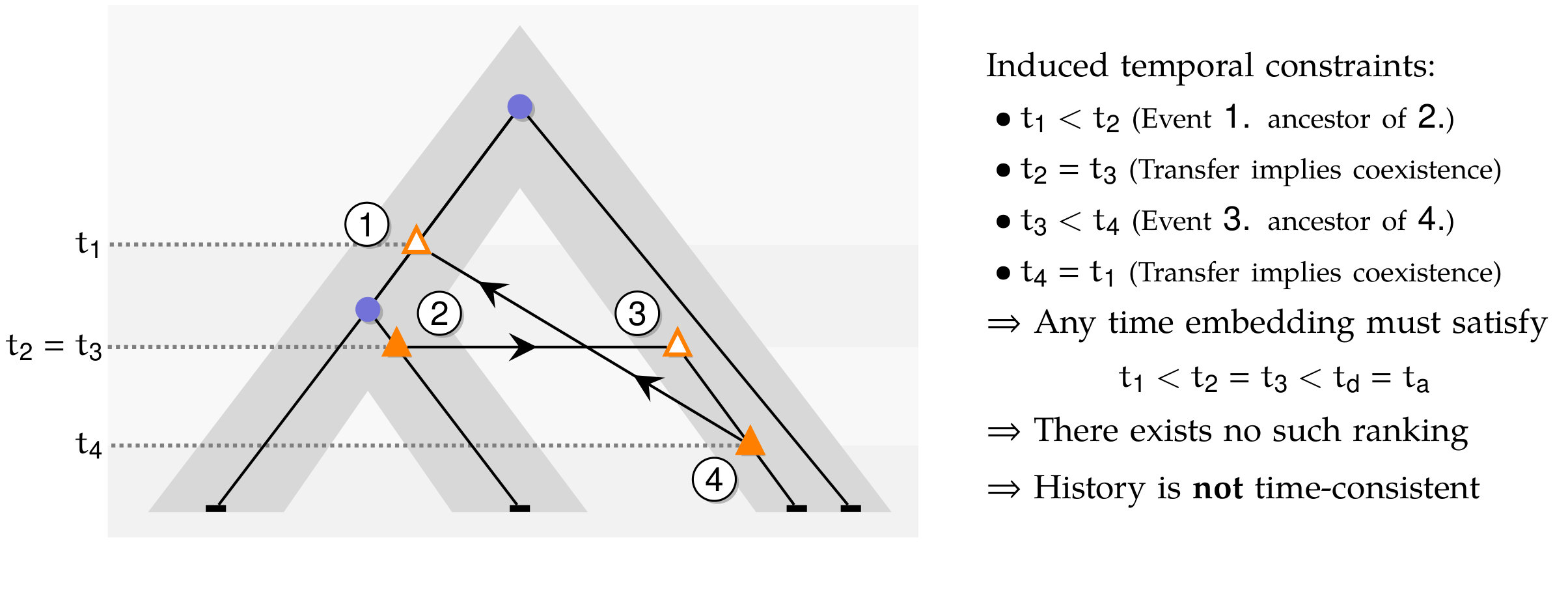 Figure 1
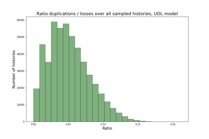 Figure 2
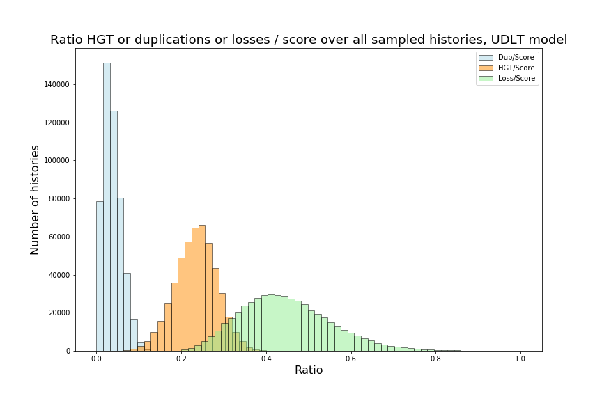 Figure 3
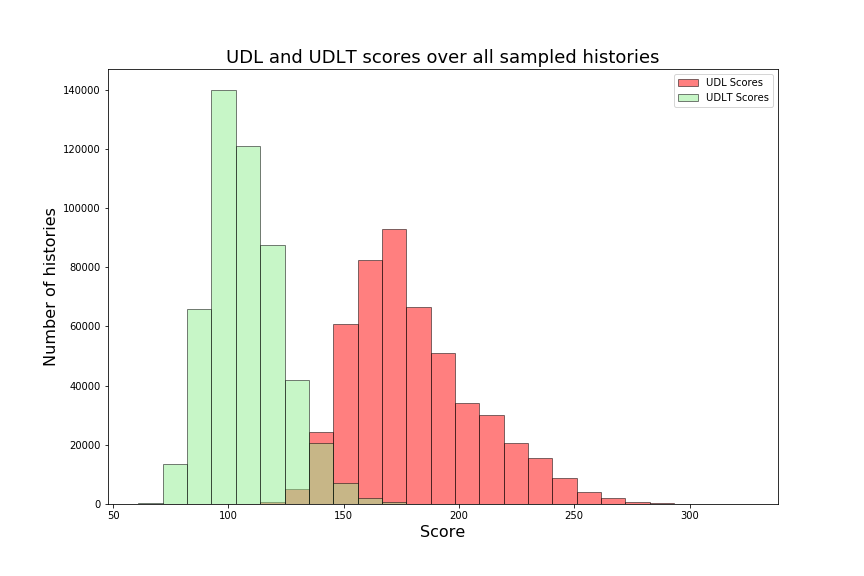 Figure 4
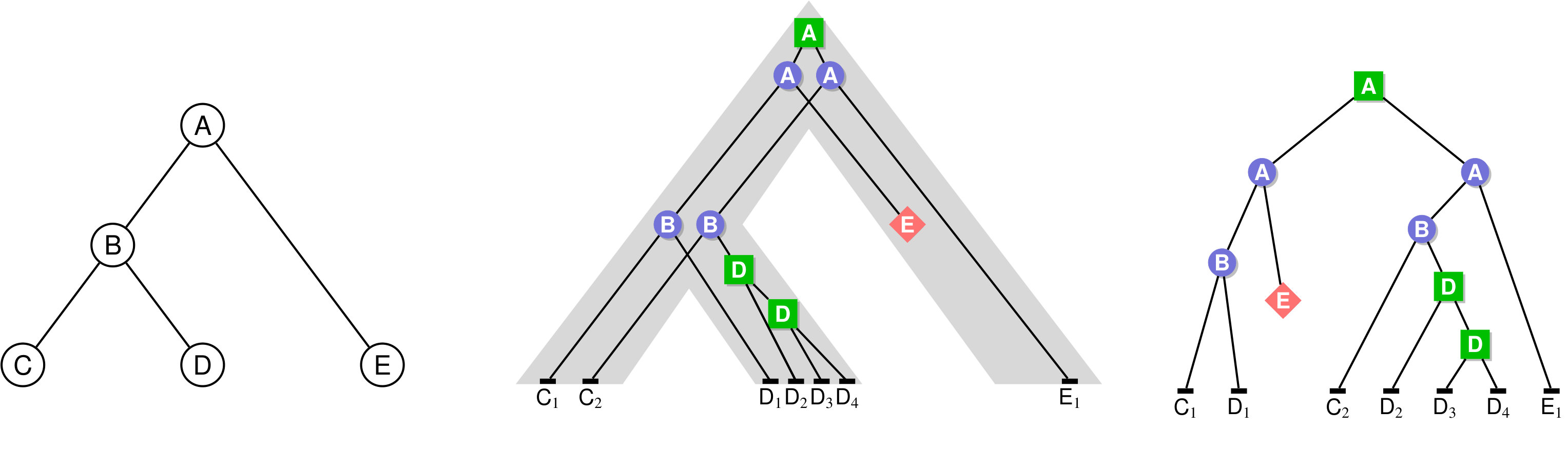 Figure 5
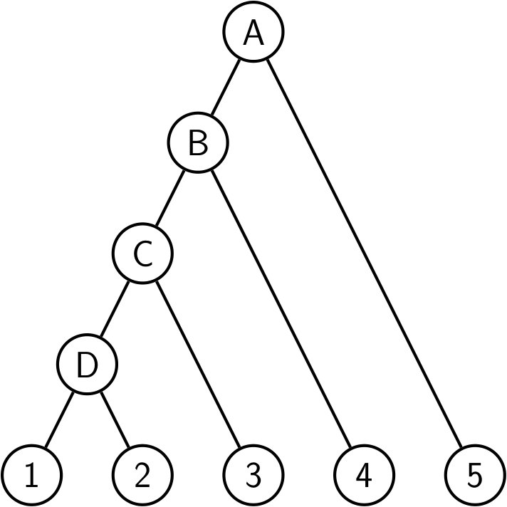 Figure 6
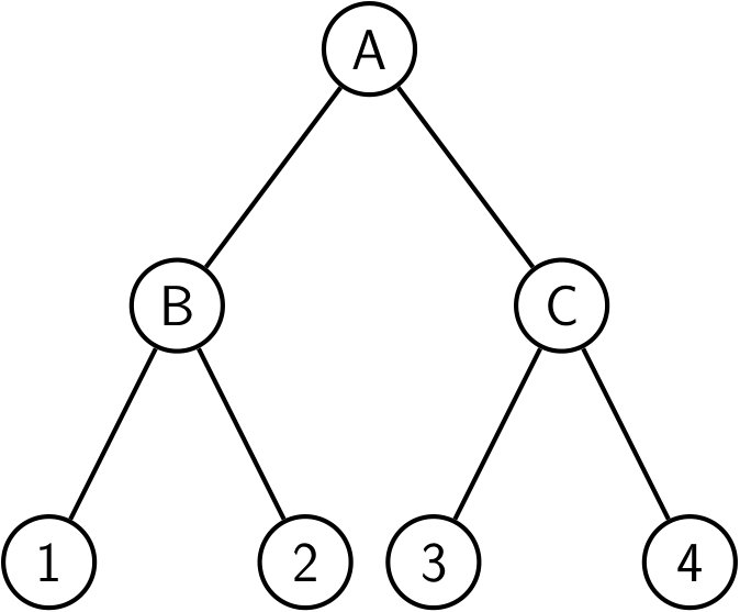 Figure 7
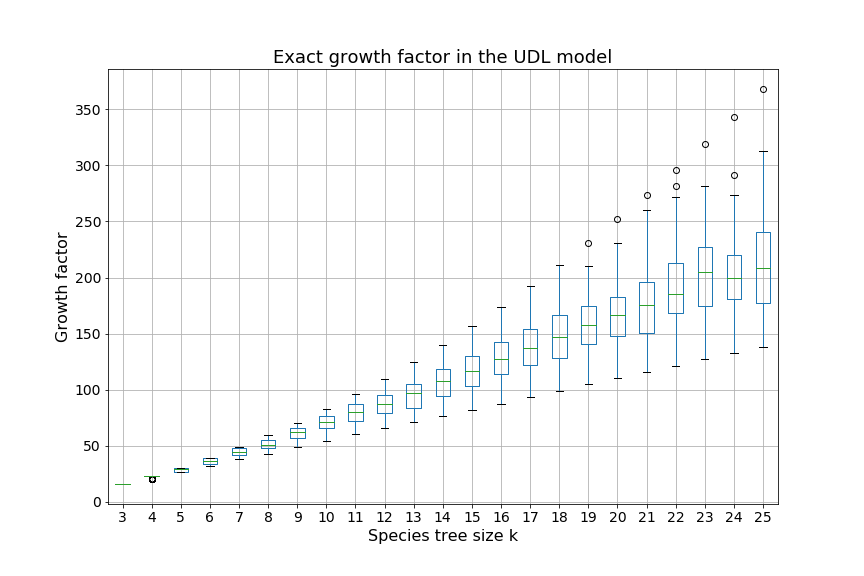 Figure 8
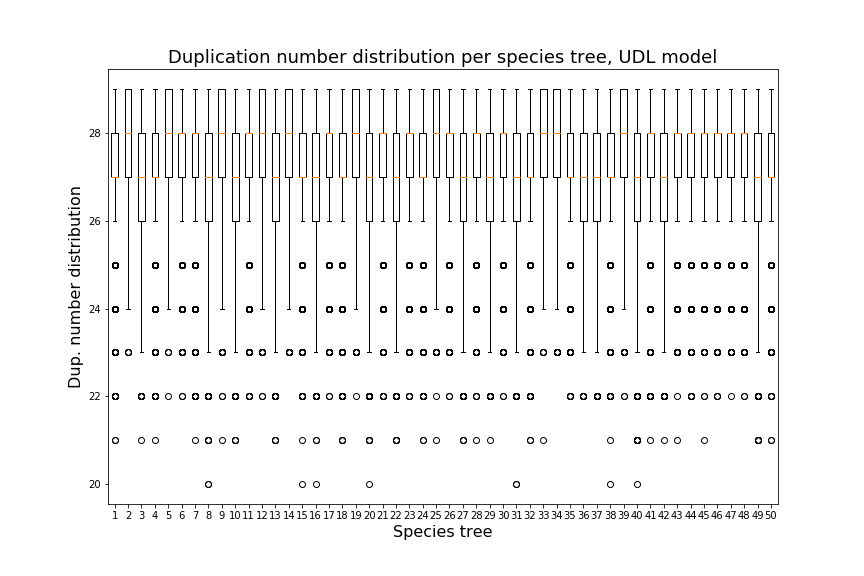 Figure 9
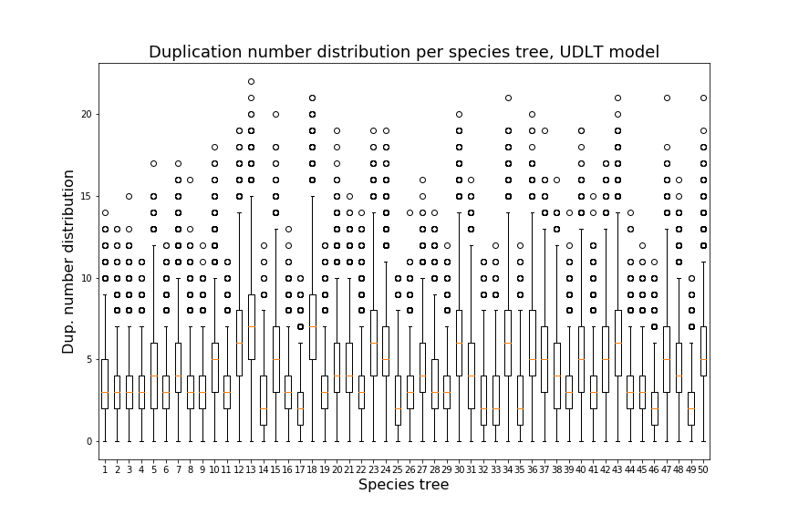 Figure 10
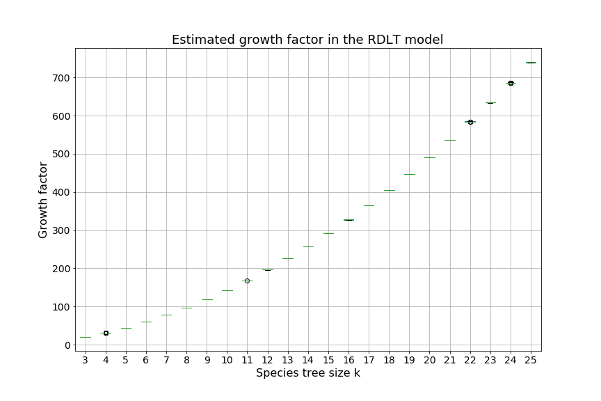 Figure 11
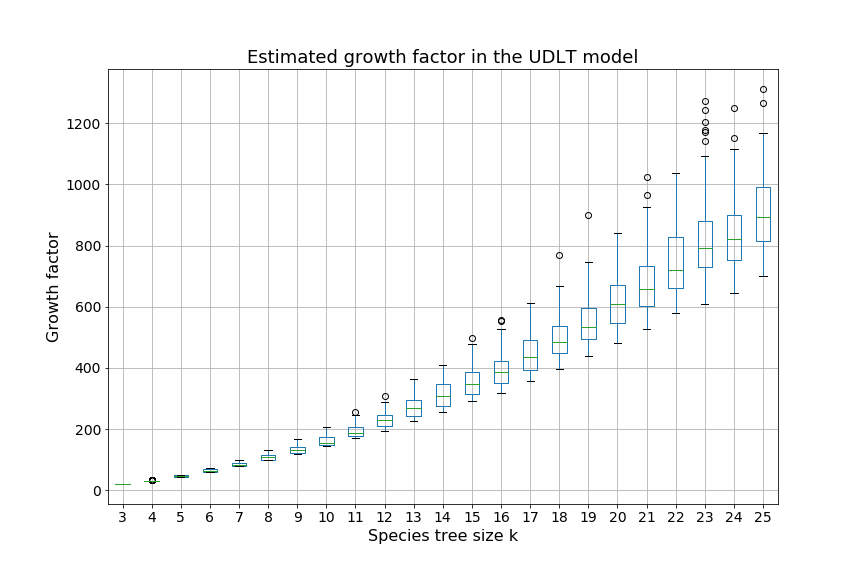 Figure 12
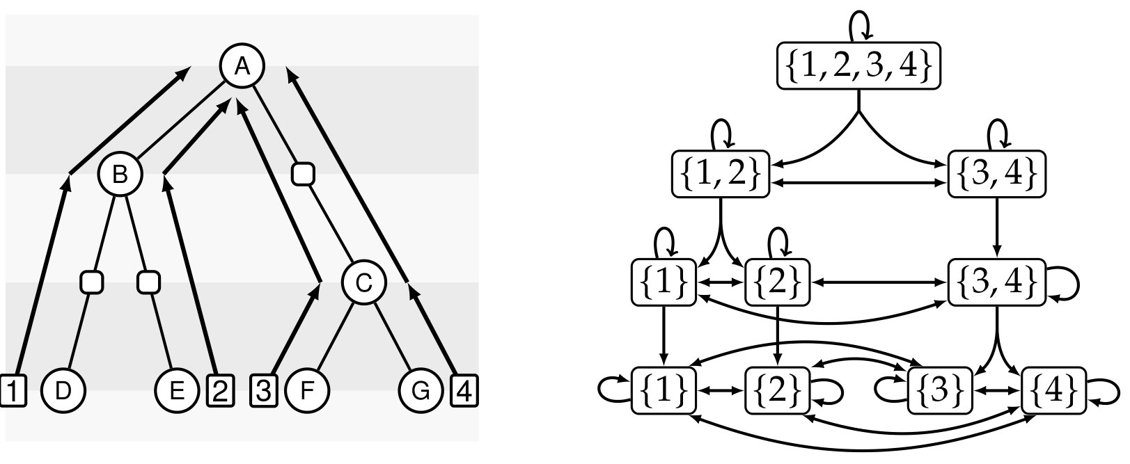 Figure 13
 Figure 14
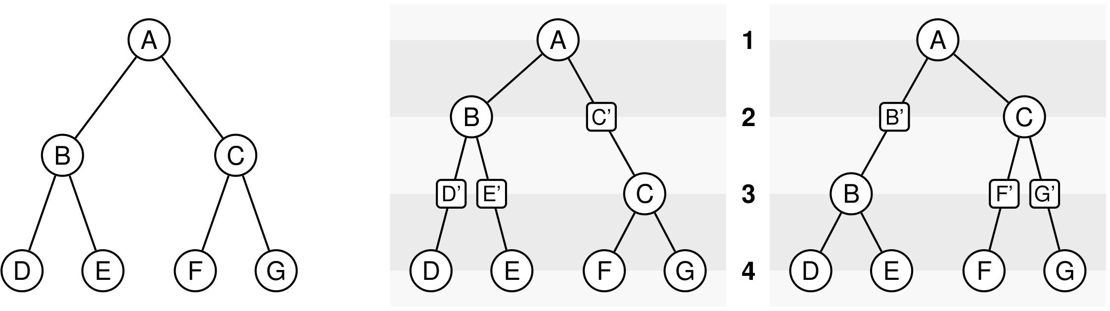 Figure 15
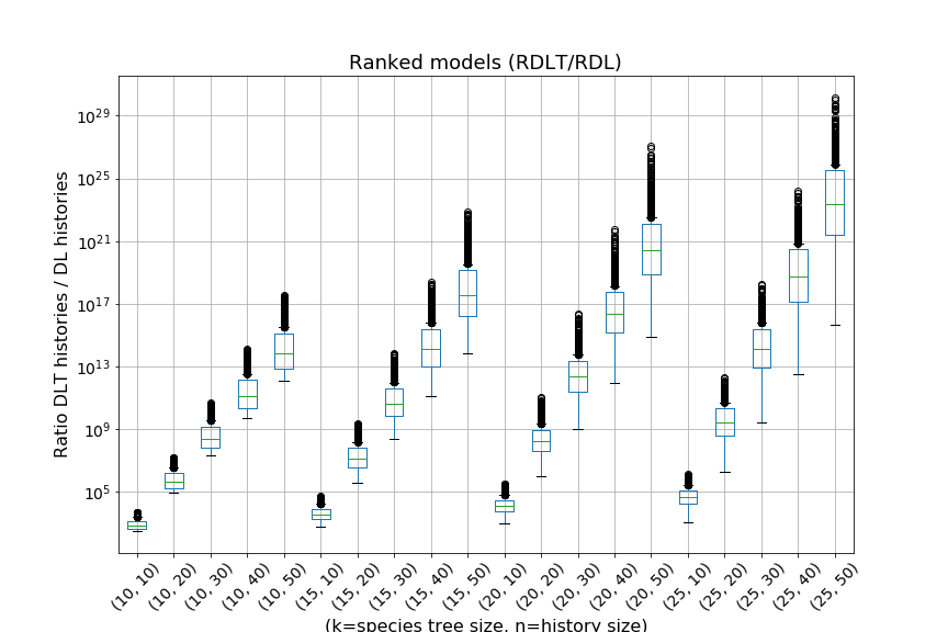 Figure 16
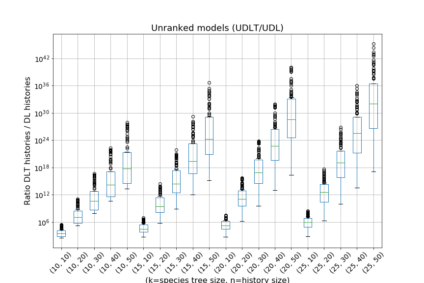 Figure 17
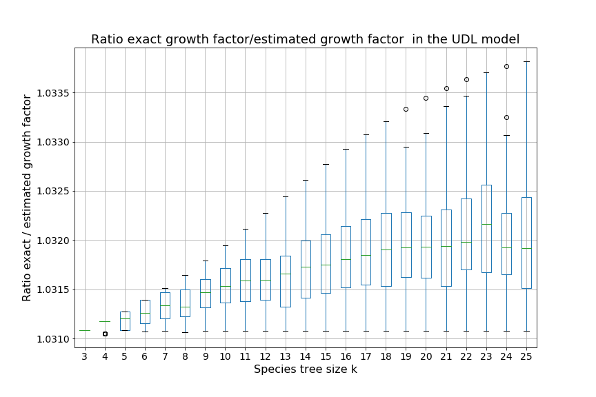 Figure 18
| if | (19) | ||||
| (20) | |||||
| if | (21) | ||||
| (22) | |||||
Peer Reviews
No public reviews on file for this paper yet. If you reviewed it on a platform where reviews are public (OpenReview, ICLR, NeurIPS, ICML), you can paste yours below so the community can read it here.
Code & Models
Videos
No videos yet. Explain this paper in a talk, walkthrough, or lecture? Add one.
11institutetext: Cedric Chauve 22institutetext: Department of Mathematics, Simon Fraser University, Burnaby (BC), Canada
LaBRI, Université de Bordeaux, Talence, France
LIX, Ecole Polytechnique, Palaiseau, France
0000-0001-9837-1878 33institutetext: Yann Ponty 44institutetext: CNRS and LIX, Ecole Polytechnique, Palaiseau, France
0000-0002-7615-3930 55institutetext: Michael Wallner 66institutetext: LaBRI, Université de Bordeaux, Talence, France
Institut für Diskrete Mathematik und Geometrie, TU Wien, Vienna, Austria
Counting and sampling gene family evolutionary histories in the duplication-loss and duplication-loss-transfer models
Cedric Chauve
Yann Ponty
Michael Wallner
Abstract
Given a set of species whose evolution is represented by a species tree, a gene family is a group of genes having evolved from a single ancestral gene. A gene family evolves along the branches of a species tree through various mechanisms, including – but not limited to – speciation (), gene duplication (), gene loss (), horizontal gene transfer (). The reconstruction of a gene tree representing the evolution of a gene family constrained by a species tree is an important problem in phylogenomics. However, unlike in the multispecies coalescent evolutionary model that considers only speciation and incomplete lineage sorting events, very little is known about the search space for gene family histories accounting for gene duplication, gene loss and horizontal gene transfer (the -model).
In this work, we introduce the notion of evolutionary histories defined as a binary ordered rooted tree describing the evolution of a gene family, constrained by a species tree in the -model. We provide formal grammars describing the set of all evolutionary histories that are compatible with a given species tree, whether it is ranked or unranked. These grammars allow us, using either analytic combinatorics or dynamic programming, to efficiently compute the number of histories of a given size, and also to generate random histories of a given size under the uniform distribution. We apply these tools to obtain exact asymptotics for the number of gene family histories for two species trees, the rooted caterpillar and the complete binary tree, as well as estimates of the range of the exponential growth factor of the number of histories for random species trees of size up to . Our results show that including horizontal gene transfer induce a dramatic increase of the number of evolutionary histories. We also show that, within ranked species trees, the number of evolutionary histories in the -model is almost independent of the species tree topology. These results establish firm foundations for the development of ensemble methods for the prediction of reconciliations.
**Mathematics Subject Classification (2000)**92B99,05A15,05A16
Keywords:
Phylogenetics, Enumerative Combinatorics, Asymptotics, Sampling Algorithms
1 Introduction
A gene tree represents the evolution of a gene family, a group of genes assumed to descend from a single ancestral gene. The reconstruction of gene trees from molecular sequence data is a central but difficult problem in computational biology. Indeed, while species are mostly expected to evolve through speciation, gene families evolve through a wider variety of mechanisms including gene duplication, gene loss, horizontal gene transfer (HGT) and incomplete lineage sorting (ILS). As a result, it is common to observe an incongruence between gene trees and species trees sysbio/Maddison97 . This discrepancy has motivated an intense research activity on the problem of reconstructing the gene tree of a gene family, conditional to a given species tree for the considered species. We refer to mmb/SzollosiD12 ; sysbio/SzollosiTDB15 for extensive reviews discussing how gene trees evolve within a species tree, describe existing models and methods for reconstructing gene trees within species trees.
In the case where a gene family contains a single gene per species, observed incongruences between a gene tree and a species tree can be analyzed through the prism of ILS in the multispecies coalescent model tree/DegnanR09 . The natural question is then to compute the probability of coalescent histories conditional to the given species tree evolution/DegnanS05 ; evolution/Wu12 ; bioinformatics/Wu16 ; bioinformatics/Wu17 . For gene families that might contain duplicate copies (or no copy) of a gene in a given species, the multispecies coalescent model is not appropriate, and gene trees need to be inferred in a model including gene duplication, gene loss and, ideally, transfers. Most methods developed to understand the evolution of gene families in this context rely on the concept of gene tree-species tree reconciliation, illustrated in Fig. 1. In this framework, given a gene tree and a species tree , one aims to embed within , often optimizing a parsimony or probabilistic criterion with regard to the considered evolutionary model.
Early reconciliation methods were developed for an evolutionary model considering only gene duplications and gene losses (the -model), and considered a parsimony criterion. This problem, introduced by Goodman et al. syszoo/GoodmanCMRM79 , is computationally tractable through dynamic programming. Extending the model to include HGT, while ensuring that HGT events are time-consistent, makes the problem of predicting of the most parsimonious reconciliation intractable in general cmb/OvadiaFCL11 ; tcbb/TofighHL11 . However, if the provided species tree is ranked, i.e. is provided with a total ordering of its internal nodes describing the order of speciation events, the reconciliation problem becomes tractable (see the discussion in bib/DoyonRDB11 ). Over the last 20 years, various efficient dynamic programming algorithms were designed to compute a parsimonious reconciliation, implemented in widely used phylogenomics packages cmb/DurandHV06 ; bioinformatics/BansalKKK18 ; bioinformatics/ScornavaccaJS15 ; bioinformatics/JacoxCSPS16 . Similar to parsimony-based methods, probabilistic reconciliation methods were first developed in a model considering only gene duplication and gene loss jacm/ArvestadLS09 ; pnas/AkerborgSAL09 ; bmcbi/GoreckiBE11 ; cmb/GoreckiE14 , before being extended to include HGTs sysbio/SzollosiRBTD13 ; sysbio/SjostrandTDASL14 .
Most methods that reconstruct a gene tree, conditional to a species tree, rely on the exploration of the space of possible evolutionary histories. It is then important to develop conceptual tools that can describe this combinatorial space and further enable its efficient exploration. This naturally raises the questions to compute the size of the space of evolutionary histories for a given gene family and a given species tree, and to be able to sample such histories. Both questions are naturally related, as precise counting results often translate into efficient sampling algorithms wilf1977unified ; flajolet1994calculus . The former (counting) question has been studied by Rosenberg et al. in the case of the multispecies coalescent model jcb/Rosenberg07 ; jcb/DisantoR15 ; tcbb/DisantoR16 ; jcb/DisantoR17 ; bmb/DisantoR17 ; jmb/DisantoR18 . However similar questions have not been explored as thoroughly for evolutionary models including gene duplication, gene loss and HGT. In this framework, dynamic programming equations aimed at computing a parsimonious reconciled gene tree can be turned into a specification of the corresponding search space tcs/GoreckiT06 ; jmb/RanwezSDB16 . This then leads to efficient algorithms for counting or sampling parsimonious reconciliations cmb/DoyonCH09 ; cmb/BansalAK13 or sampling reconciled gene trees under the Boltzmann probability distribution bioinformatics/JacoxCSPS16 . However, to the best of our knowledge, such questions have not been considered in the case where a gene tree is not specified at first, i.e. we are only given a species tree and gene family.
This paper provides analytic and algorithmic answers to those questions. We show that, for a given species tree, whether ranked or unranked, the space of all possible evolutionary histories of a fixed size in the -model can be described using a formal grammar. This allows us to compute, in polynomial time and space, for given species tree and gene family size, the number of evolutionary histories of this size conditional to the given species tree, as well as to sample among these histories under the uniform probability. Using these algorithms, we can provide estimates of the exponential growth factor of the number of histories in the -model and -model. We show that, as expected, including HGT in a model results in an exponential increase of the number of histories. We also notice that with a ranked species tree, the exponential growth factor of the number of histories in the -model seems to be almost independent of the chosen species tree. Finally, using enumerative and analytic combinatorics, we provide exact values for the asymptotic number of histories for two specific species tree: the rooted caterpillar tree and the rooted complete binary tree.
2 Model: gene families evolutionary histories
In this section, we introduce the combinatorial objects modeling the evolution of a gene family within a given species tree, that we call histories.
Preliminaries on trees.
For a given rooted tree111In the present work we consider only rooted trees. , we say it is uniquely labeled if every node has a label, and no two nodes have the same label. For a node in , we denote by the subtree of rooted at . In this work, we consider only binary and unary-binary trees: in a binary tree, every internal node has exactly two children, while in a unary-binary tree, an internal node can have either one child or two children. If a uniquely labeled tree is unordered we take advantage of the nodes labeling to see it as an ordered tree, with the two children of an internal node being ordered from left to right in increasing order of their labels; so from now on all trees we consider are ordered. If an internal node of a tree is binary, we denote by the left child of and by its right child; if is unary, i.e. has a single child, we denote it by . We denote by the root of . For a node of , we denote by its parent in . The size of a tree is the number of its leaves.
A rooted tree describes a partial order on the set of its nodes, and two nodes are said to be comparable if one is an ancestor of the other one and incomparable otherwise. For a node , we denote by the set of nodes that are incomparable with .
Ranked trees.
A ranking of a tree of size is a mapping from the nodes of to such that (1) if is a leaf, (2) if and are internal nodes, and (3) if is an ancestor of . A tree augmented with a ranking is called a ranked tree; in our context it models the evolution of a set of species, the ranking providing the relative order of speciation events, under the assumption that no two speciations can occur at the same time.
Given a binary tree and a ranking , we define an unranked unary-binary tree that encodes the ranking information as follows: for each internal node , considered iteratively in increasing ranking order, and for every edge such that , we subdivide the edge into two edges and , so adding a unary node on this edge. We denote by the set of all unary nodes created in this way and we call this set of nodes together with a time slice. Additionally, we also define the set of all leaves as a time slice (see Figure 2). Note that in this way we create different time slices which correspond to the different values of the ranking. We modify the notion of incomparability for such unary-binary trees as follows: for a node , .
Gene Families Evolutionary Histories.
The objects we study in this work model the evolution of a gene family within a species tree. A species tree, which will be denoted by from now on, is a uniquely labeled rooted binary tree that represents the evolution of a set of species through speciation events; can be either unranked or ranked. A gene family evolves within from a single ancestral gene, present in the species , through four possible kinds of evolutionary events:
- •
Speciation : a gene present in species has two descendant genes present in species and present in species .
- •
Duplication : a gene present in species is duplicated, with a new copy of appearing in species ; is said to be the original gene while is the novel gene.
- •
Loss : a gene present in species has exactly one descendant either in or in , implying that after a speciation at species , exactly one of the two resulting genes is lost along the branch toward either or .
- •
Horizontal Gene Transfer (HGT): this is similar to a duplication but the novel copy, denoted here, appears in a species different from and incomparable with , called the receiver of the HGT, while is called the donor of the HGT. If is ranked, with ranking , the receiver species is required to exist at the same time as , i.e. to satisfy two ranking constraints, .
Definition 1
An evolutionary history for a gene family within a species tree is a unary-binary ordered rooted tree together with two mappings and satisfying the following constraints:
- •
if is a leaf, ;
- •
if is internal and binary, ;
- •
if is internal and unary then 222Note that technically the event associated to a unary node in the species tree is not speciation in the biological meaning, but we chose to label it as such for expository reasons.;
- •
if and is binary then and ;
- •
if and is unary then ;
- •
if then ;
- •
if then and .
The size of a history is the number of leaves such that .
Intuitively, this definition states that a history is represented by a tree where each node corresponds to a gene present in a species, either extant or ancestral (the mapping ), and each ancestral gene either was lost () or evolved toward extant genes through a duplication (), an HGT to an incomparable receiver species () or a speciation (), while extant genes belong to extant species; the constraints on the species mapping ensure that this history can be embedded within as illustrated in Figure 1.
By convention, for duplications, we consider that the novel copy of a gene is its right child , representing the original copy. Histories considered by the -model, which allows both duplications and losses (resp. duplications, losses and HGTs), are called -histories (resp. -histories).
Remark 1
By modeling the evolution of a gene family with ordered trees we differ from the classical notion of reconciliation, that also models the evolution of a gene family but considers that when a gene duplication occurs, the original gene and the novel gene are indistinguishable. As a result, the children of a duplication are ordered within a history, whereas they are not in a reconciliation.
Remark 2
Gene losses are modeled as speciation events with one disappearing gene. As a consequence, we can not have a duplication or a HGT that results in one of the resulting two gene copies being lost. This is necessary to avoid creating an infinite number of histories of a given size, due to an arbitrary number of duplications within a species, each followed by a loss, or an arbitrary long sequence of HGT, again each followed by a loss, leading to at most one extant gene.
Time Consistency of -histories.
Given an unranked species tree , a -history as defined above is time inconsistent if there exists a gene belonging to a species such that one of its ancestors belongs to a species and one of its descendants belongs to a species ancestral to . This pattern can be observed due to the fact that, in the definition of a -history, the choice of the receiver species of an HGT of gene belonging to species is not restricted to the set of species that are also incomparable with all species containing genes that are ancestral to ; see Figure 3 for an illustration.
The problem of computing gene family evolutionary scenarios that are both parsimonious and time-consistent has been shown to be intractable when such scenarios are modeled by reconciliations with an unranked species tree tcbb/TofighHL11 ; cmb/OvadiaFCL11 , while, when the provided species tree is ranked, the problem becomes tractable (see bib/DoyonRDB11 and references therein). Similarly, when is ranked, we can ensure time-consistency of evolutionary histories, by requiring that the donor and receiver of any HGT belong to the same time slice in , i.e. the receiver of an HGT of a gene belonging to a species belongs to .
3 Methods
Our results (counting and sampling algorithms) are based on the design of formal grammars specifying, for a given species tree , the combinatorial families of -histories and -histories constrained by . These grammars are then used as templates to design dynamic programming algorithms for counting and sampling (under the uniform distribution) the number of histories of a fixed size. Moreover, these grammars are amenable to techniques of analytic combinatorics that allow us to compute the asymptotic growth constant for the number of histories. We first describe our grammars, then the counting and sampling algorithms, and finally the asymptotic analysis of these grammars.
3.1 General grammars specifying -histories and -histories
In this section we describe grammars specifying histories evolving within a species tree using the formalism developed in comb/FlajoletS09 . We describe grammars for -histories, for both an unranked and a ranked species tree; these grammars can then be specialized into grammars for -histories by omitting the rules related to HGT.
Let be a species tree. If is unranked, it is a binary tree, otherwise, if it comes with a ranking , we consider the unary-binary species tree . So in the statements below, when mentioning a ranked species tree we mean the unary-binary tree defined by the ranking.
We denote by the set of -histories for the tree . In the most general setting, following comb/FlajoletS09 , these grammars contain both terminal symbols, corresponding to atomic elements of the histories (nodes) and non-terminal symbols, corresponding to combinatorial operators applied to sets of histories. We use the non-terminal to encode a gene present in extant species ; moreover, we use for a gene lost at species , for a duplication at species and for a HGT with donor species . We consider two combinatorial operators, the disjoint union and the Cartesian product.
Theorem 3.1
The set defined by the grammar below specifies the set of all -histories for a species tree .
[TABLE]
where is the set of nodes that are incomparable with in . The set of -histories is specified by the same grammar where rule (6) is removed and the terms are removed from rules (1) and (2).
Proof
The grammar follows the definition of histories, Definition 1. Rule (1) simply states that the root (i.e. the first evolutionary event of the history) of a -history within the subtree , assuming it is not reduced to a leaf, is either a speciation, a duplication or a transfer of the ancestral gene present in species : non-terminal , and represent respectively these three subsets of . Rule (2) addresses the case where is composed of a single leaf, in which case there can not be a speciation event, but a history reduced to a single gene in species .
Rule (3) describes a speciation event at species . The ancestral gene can either evolve into a gene in each of the two children of (first term of the union) or into a gene in a single child of due to a gene loss in the other child of . In the case where is unary (due to being a node created by the time slicing in a ranked ), the ancestral gene evolves into a copy in the unique child of .
Rule (5) addresses the case of a duplication. It results in two ordered independent histories starting at species : the first one being the history of the original copy of the starting ancestral gene and the second one the history rooted at the novel gene created by the duplication.
Last, Rule (6) addresses the case of histories starting by a HGT. Generally, a HGT has a structure similar to a duplication but for the fact that the novel gene appears in a species that is incomparable with .
These various rules cover all cases for describing the possible first event of a history and are mutually exclusive, thus providing a complete recursive specification of -histories for a given species tree . It follows immediately that removing the rule and non-terminals associated to HGT gives a grammar specifying -histories for . ∎
Remark 3
The above grammar can be greatly simplified if one is interested only in the number of histories of a given size, as opposed to the specific species where gene duplication, gene loss and HGT events occur and the precise gene content of extant species. In this case, one simply identifies all non-terminals (resp. , , ) to a single variable (resp. , , ). From now, we follow this approach.
3.2 Counting and sampling algorithms
The grammar defined above can naturally be turned into a dynamic programming algorithm computing the number of histories of a given size. This algorithm computes tables where, for a given node of and a given history size , (respectively, , , ) is the number of -histories of size evolving within (respectively, starting with a duplication, a speciation, and an HGT). We illustrate this in the case of -histories with an unranked species tree .
[TABLE]
A random generation algorithm can then be adapted from the counting recurrences, resulting in an instance of the so-called recursive method wilf1977unified . Right-hand sides of the counting equation are split into sums of multiplicative terms. Starting from the initial state , the algorithm randomly chooses a term from the right-hand side of the current state, with probability proportional to its contribution to the counting. When the selected term is a multiplication of two terms, the length needs to be distributed across the two terms, and a pair of lengths , is chosen with probability proportional to the associated count. For the sake of performances, the various alternatives can be explored in Boustrophedon order, ensuring an overall worst-case complexity flajolet1994calculus . Recursive calls are then performed over the states associated with the chosen term, until a leaf is chosen (term ). This leads to the following result.
Theorem 3.2
The number of histories of size constrained by a species tree of size can be computed in polynomial time and space , where and both depend on the model ( or ) and the ranked/unranked nature of the species tree, as summarized in Table 1.
The uniform random generation of histories of size can be performed in time .
3.3 Asymptotic number of histories in the -model
The grammar given in Theorem 3.1 defines a combinatorial specification of the set of histories for a given species tree in a given evolutionary model. In this section, we derive the asymptotic number of histories in the -model and use it later on two specific species trees: the caterpillar and complete binary trees. The following theorem is the main result of this section and describes their asymptotic growth for tending to infinity.
Theorem 3.3
For any given species tree , the number of histories in the unranked -model given by Equations (1)-(5) is, for large , equal to
[TABLE]
for explicitly computable constants and .
In the remainder of this section we prove this theorem. The grammars are amenable to enumerative and analytic combinatorics techniques. We follow the general approach presented in Flajolet and Sedgewick comb/FlajoletS09 and Drmota comb/Drmota97 . It consists mainly in translating the combinatorial specification of a combinatorial family into equations defining its counting generating function. Then, its analytic properties lead to precise asymptotic formulas for its coefficients. We provide an overview of this approach in Example 1.
Example 1
Consider the class of rooted binary trees . Such a tree is either a leaf, or it consists of a root with two children which are also each roots of binary trees. Let us mark each leaf with the variable . Then, the grammar is given by
[TABLE]
Let be the number of binary trees with leaves and let be the counting generating function of binary trees. The symbolic method (comb/FlajoletS09, , Part A) translates this grammar directly into an equation for the generating function:
[TABLE]
Its generating function is thus given by
The general method of singularity analysis from analytic combinatorics (comb/FlajoletS09, , Chapter VI) allows us to directly get the asymptotics of the coefficients. First, by the Cauchy–Hadamard theorem, the asymptotic growth is directly connected with the dominant singularities (and the radius of convergence) of the counting generating function. Here, the generating function becomes singular at , which is also the unique singular point. Hence, the coefficients grow like . Second, using transfer theorems of analytic combinatorics (comb/FlajoletS09, , Theorem VI.1 and Theorem VI.3) we also get the subexponential terms and recover the well-known result for Catalan numbers (see OEIS A000108 comb/Sloane ):
[TABLE]
for .
We will now describe this approach applied to the grammar specifying the -histories with an unranked species tree . Let be the number of -histories of consisting of genes represented in the generating function by the formal variable . We define the counting generating functions
[TABLE]
The coefficients represent the number of histories of size associated with the species tree independent on the number of losses or duplications. These generating functions (one per species of ) are strongly related to the generating function of binary trees introduced in Example 1.
Lemma 1
For a given species tree the counting generating function for histories in the unranked -model is defined by the system of functional equations
[TABLE]
over all nodes of , where
[TABLE]
Proof
The symbolic method (comb/FlajoletS09, , Part A) translates the unranked -grammar of Equations (1)-(5) directly into a system of equations for the generating functions. We get
[TABLE]
Comparing these equations with the one for binary trees from Equation (13) the claim follows. ∎
The advantage of a generating function approach is that we are able to identify the subexponential growth as , and that we are able to explicitly compute exponential growth and the constant for a fixed species tree . We will compute the involved constants explicitly for the caterpillar tree in Section 4.1.1 and for the complete binary tree in Section 4.1.2.
By basic principles of analytic combinatorics, the asymptotic growth of a counting sequence is directly related to the radius of convergence of the corresponding generating function. In particular, its dominant singularity (i.e. the one closest to the origin) defines its asymptotic growth. By the construction in terms of nested radicals, the generating function is singular if and only if at least one of its radicals becomes zero. Therefore, we make the structure of nested radicals visible. Writing the explicit form of the outermost in (14) gives
[TABLE]
Then, the radicands satisfy the following recurrence
[TABLE]
The recurrence can be used to determine the nature of the radii of convergence. For a node we define as the radius of convergence of .
Lemma 2
Let be the parent of in . Then, and with if is a leaf. Furthermore, is the only radicand that vanishes at and is a simple root.
Proof
By combinatorial construction is built of nested radicals and does not include any poles. Therefore, its dominant singularity must be at a point where (at least) one of its radicands vanishes.
We continue by induction on the depth of the subtree with root given by . The depth is the longest path from the root to any leaf. As a first step, we prove that and that . For a leaf it is clear from Relation (17) that and that .
Next, let and be the children of such that . By the induction hypothesis we directly get
[TABLE]
In order to continue, note that is monotonically decreasing on , because from the decomposition in (16) and (15) we see that
[TABLE]
for certain non-negative numbers .
By the induction hypothesis and Relation (17), is a continuous function on . Hence, we get
[TABLE]
Thus, on the one hand, by the intermediate value theorem must have at least one zero in the interval . On the other hand, as is monotonically decreasing it has at most one zero in . Hence, this zero is equal to .
Finally, the above reasoning implies that among the nested radicals of the outermost one is the first one that vanishes, and no other radical vanishes at the same time. Thus, is the radius of convergence of . Moreover, by (18) we see that the derivative has non-positive coefficients. Hence, is a simple root. ∎
Let us shortly digress and discuss in a more general context how to numerically compute the exponential growth for the coefficients of the generating function with the fastest exponential growth that is defined by a system of functional equations involving generating functions of the form
[TABLE]
where the are polynomials with non-negative integer coefficients in variables. Note that the grammar given in Theorem 3.1 is of this shape. In order to decide which of the ’s has this specific exponential growth, further information on the problem, like in our case given by Lemma 2, is needed. By Banach’s fixed point theorem, these equations admit a unique solution vector with respect to the formal topology (comb/FlajoletS09, , Section A.5). Furthermore, each has non-negative coefficients in its expansion around [math] (which is already clear from the combinatorial nature of the problem). Then, the multivariate version of the implicit function theorem implies that each of them has a non-zero radius of convergence which we call . By Pringsheim’s Theorem (comb/FlajoletS09, , Theorem IV.6), is a singularity of . Moreover, as is an ordinary generating function of an infinite combinatorial class, we must have . Finally, in order to compute the radius of convergence, we find the minimal point where the implicit function theorem fails. To be more precise, we numerically compute solutions and of the following system
[TABLE]
where is the Kronecker symbol: , and for .
Remark 4
The unranked -grammars lead to the following specific shape
[TABLE]
Hence, we get We actually know by Lemma 2 that the outermost square-root vanishes, which gives . Additionally, we can also directly deduce from this system that .
In the unranked -model the system looks like
[TABLE]
where the last equation is the only one involving , as the root can not be a receiver of an HGT. Note that the subsystem of the first equations is strongly connected and but still not satisfies the -properness condition (i.e. it is no contraction in the formal topology) of the Drmota–Lalley–Woods Theorem (comb/FlajoletS09, , Theorem VII.6) which would directly imply a square root singularity. Thus, we conjecture that the dominant singularity still comes solely from the outermost square root of implying .
In the ranked -model we are dealing with blocks of strongly connected components that correspond to the time slices. Note that the root is contained in a singleton time slice. Experiments suggest the same behavior as in the previous cases.
However, one thing is for sure in all models: we always have for all other subtrees with root of the species tree. Hence, there will be always a dominant minimal singularity in that can be (numerically) computed. Note however, that the determinant computation soon becomes extremely heavy.
After determining the radius of convergence, we must determine the number of singularities on it. As shown in the case of -terms in (comb/BodiniGGG18, , Lemma 8) there can only be one dominant singularity . Let us quickly repeat this argument here. Assume that there exists a root of the same modules. Substituting this value into from (18) gives
[TABLE]
which can only hold if whenever . Now, due to we have . Hence, is the unique dominant real singularity of .
Combining the previous results, we have shown for a family of constants the following local singular expansion
[TABLE]
The fact that has a simple root at shows that . Then, by transfer theorems of analytic combinatorics (comb/FlajoletS09, , Theorem VI.1 and Theorem VI.3), we get the claimed asymptotic expansion of Equation (12), where and this ends the proof of Theorem 3.3.
Remark 5
There are several possible extensions of the previous approach. First of all, it is straightforward to extend it to the ranked -model. In that case one only needs to incorporate unary nodes arising from the time slices. Second, an extension to the -model is also possible, yet the computations are more involved as the binary tree structure leading to Lemma 1 does not hold anymore. However, it can still be modeled with colored binary trees, where the number of colors depends on the size of the set of incomparable nodes (in the the current time slice). Third, it is also possible to consider the distribution of certain parameters, such as the number of gene losses, or the number of gene duplications, see e.g. for related results in lattice paths and trees comb/BonaF09 ; comb/GittenbergerJW18 ; comb/BanderierW17 . Using multivariate generating functions and marking each such event by an additional variable like in the general grammar of Theorem 3.1, the above results for the -model directly generalize to the respective ones on multivariate generating functions. All these generalizations are interesting future research directions.
The counting and sampling algorithms described above have been implemented in Python, and are available at https://github.com/cchauve/DLTcount.
4 Results
Over the next two sections, we will apply Theorem 3.3 to the special cases of the caterpillar and complete species tree in the unranked -model, and explicitly determine the constants involved in the asymptotic expansion. Then, we apply our dynamic programming counting and sampling algorithms to study properties of random evolutionary histories.
4.1 Asymptotic expansion for extremal species trees in the -model
Our experimental results (Section 4.2) suggest that for a given , the species trees having the largest (resp. smallest) number of -histories are respectively the caterpillar tree and the balanced binary tree (Conjecture 1), defined below. In the present section, our main results are the explicit computation of the asymptotic growth and the leading constant of Theorem 3.3 for the caterpillar species tree (Propositions 1 and 2) and for the complete binary species tree, the special case of balanced trees when is a power of (Propositions 3 and 4, see also Table 4.1).
The rooted caterpillar tree can be defined as follows: is the tree reduced to a single leaf, while () is the tree formed by a left subtree equal to and a right subtree equal to . Observe that every subtree of a caterpillar tree is itself a caterpillar tree, see Figure 4.
The complete binary tree with leaves can be defined as follows: is the tree reduced to a single leaf, while () is the tree formed by a left and a right subtree both equal to . Observe again that every subtree is itself a complete binary tree, see Figure 4. The complete binary tree is a special case of the class of balanced trees, defined as trees where, for each node, the number of leaves in the left subtree differs from the number of leaves in the right subtree by at most one. Complete binary trees are the only balanced trees in which the number of leaves is a power of two.
We can observe that the number of -histories grows much faster for the caterpillar tree than for the complete binary tree. This is actually unsurprising given that the number of -histories can be linked to the size of the grammar, which itself depends on the structure of the species tree. More precisely, the size of the grammar depends on the number of unique subtrees of the considered species tree . Each such subtree may be identified by its root and corresponds to one set of rules (1)-(6), while subtrees having the same topology lead to isomorphic subgrammars with the same counting generating functions. The caterpillar (resp. complete binary) tree has the largest (resp. smallest) number of unique subtrees within the set of species trees of the same size (when is a power of for the complete binary tree), compare also Table 4.1.
The reference list from the paper itself. Each links out to its DOI / PubMed record.
- 1[1] Ö. Åkerborg, B. Sennblad, L. Arvestad, and J. Lagergren. Simultaneous bayesian gene tree reconstruction and reconciliation analysis. Proceedings of the National Academy of Sciences , 106(14):5714–5719, 2009.
- 2[2] L. Arvestad, J. Lagergren, and B. Sennblad. The gene evolution model and computing its associated probabilities. Journal of the ACM , 56(2):7:1–7:44, 2009.
- 3[3] Y. ban Chan, V. Ranwez, and C. Scornavacca. Inferring incomplete lineage sorting, duplications, transfers and losses with reconciliations. Journal of Theoretical Biology , 432:1–13, 2017.
- 4[4] C. Banderier and M. Wallner. Lattice paths with catastrophes. Discrete Mathematics & Theoretical Computer Science , Vol 19 no. 1, Sept. 2017. Full version of extended abstract with the same title appeared in the Proceedings of conference on Random Generation of Combinatorial Structures – {GAS Com} 2016.
- 5[5] M. S. Bansal, E. J. Alm, and M. Kellis. Reconciliation revisited: Handling multiple optima when reconciling with duplication, transfer, and loss. Journal of Computational Biology , 20(10):738–754, 2013.
- 6[6] M. S. Bansal, M. Kellis, M. Kordi, and S. Kundu. Ranger-dtl 2.0: rigorous reconstruction of gene-family evolution by duplication, transfer and loss. Bioinformatics , 34(18):3214–3216, 2018.
- 7[7] M. Bendkowski, O. Bodini, and S. Dovgal. Polynomial tuning of multiparametric combinatorial samplers. In Proceedings of the Fifteenth Workshop on Analytic Algorithmics and Combinatorics, ANALCO 2018, New Orleans, LA, USA, January 8-9, 2018. , pages 92–106. SIAM, 2018.
- 8[8] O. Bodini, D. Gardy, B. Gittenberger, and Z. Gołębiewski. On the number of unary-binary tree-like structures with restrictions on the unary height. Annals of Combinatorics , 22(1):45–91, 2018.
