Orthogonal sequences constructed from quasi-orthogonal ultraspherical polynomials
Oksana Bihun, Kathy Driver

TL;DR
This paper explores the construction of orthogonal sequences from interlacing zeros of ultraspherical polynomials, providing an algorithm and analyzing the zeros' behavior for different parameter ranges.
Contribution
It introduces a novel algorithm for generating orthogonal sequences from ultraspherical polynomials' interlacing zeros, addressing a question posed by Mourad Ismail.
Findings
Zeros of constructed polynomials differ significantly for certain parameter ranges.
The shape of zero curves varies with the parameter λ, showing distinct behaviors.
The method extends the understanding of orthogonal sequences related to ultraspherical polynomials.
Abstract
Let and , be two sets of real, distinct points satisfying the interlacing property Wendroff proved that if and , then and can be embedded in a non-unique monic orthogonal sequence We investigate a question raised by Mourad Ismail at OPSFA 2015 as to the nature and properties of orthogonal sequences generated by applying Wendroff's Theorem to the interlacing zeros of and , where is a sequence of monic ultraspherical polynomials and We…
Click any figure to enlarge with its caption.
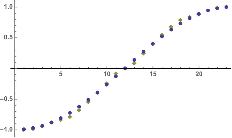 Figure 1
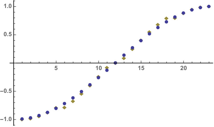 Figure 2
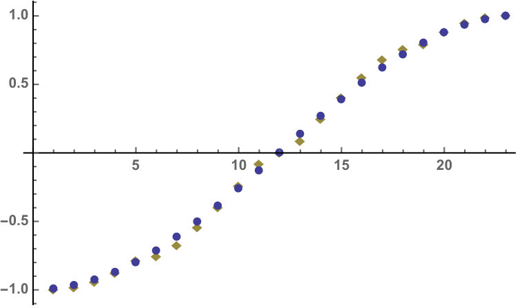 Figure 3
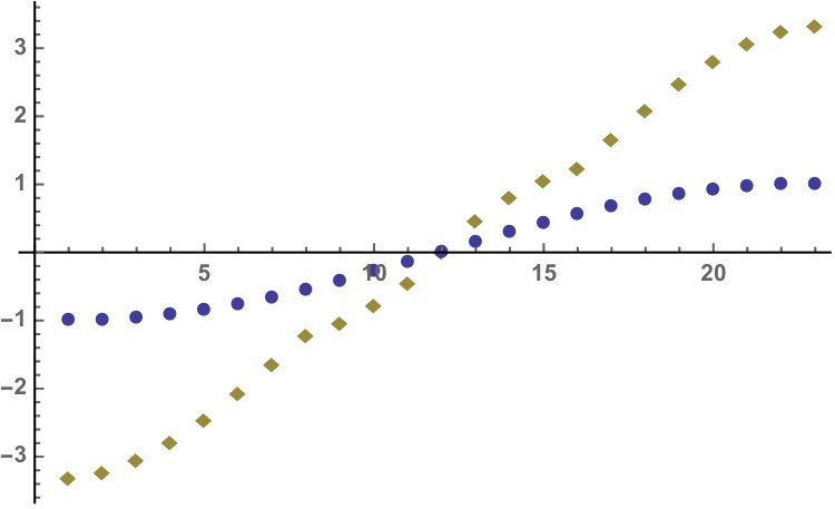 Figure 4
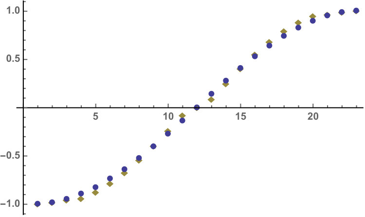 Figure 5
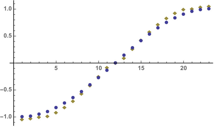 Figure 6
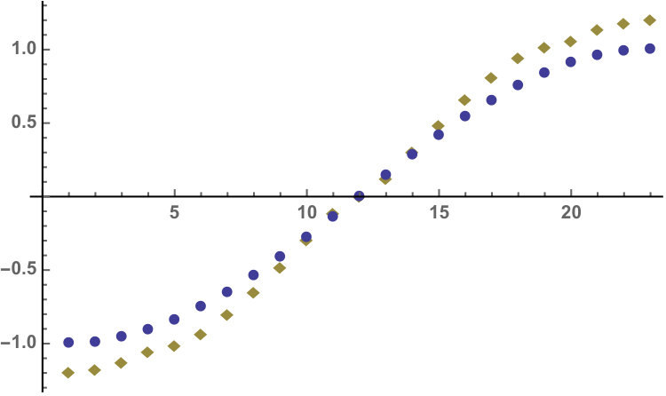 Figure 7
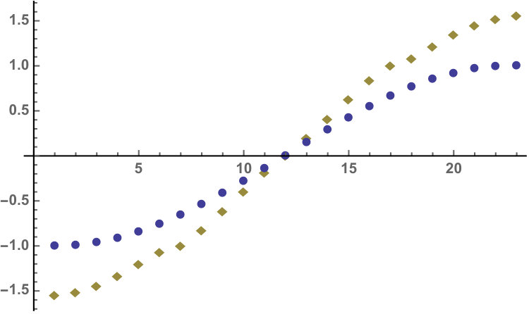 Figure 8
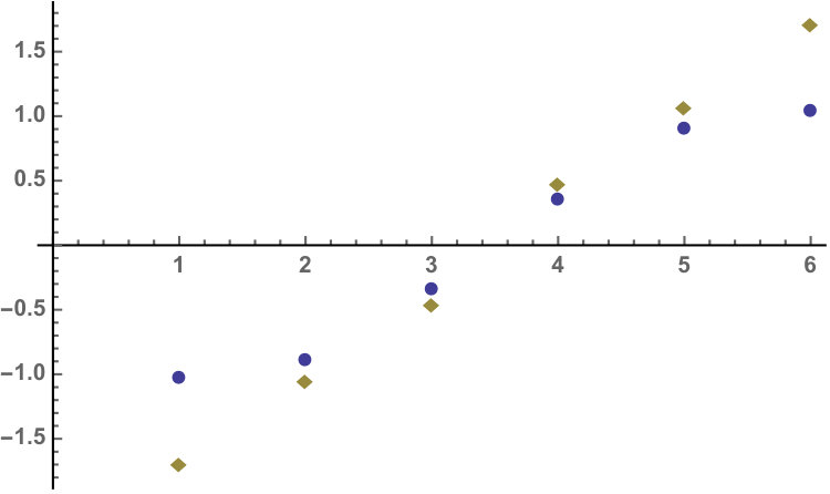 Figure 9
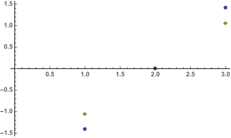 Figure 10
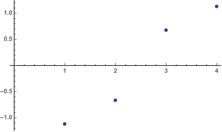 Figure 11
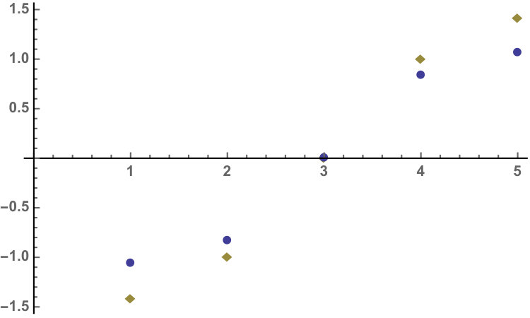 Figure 12
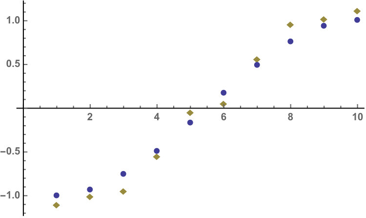 Figure 13
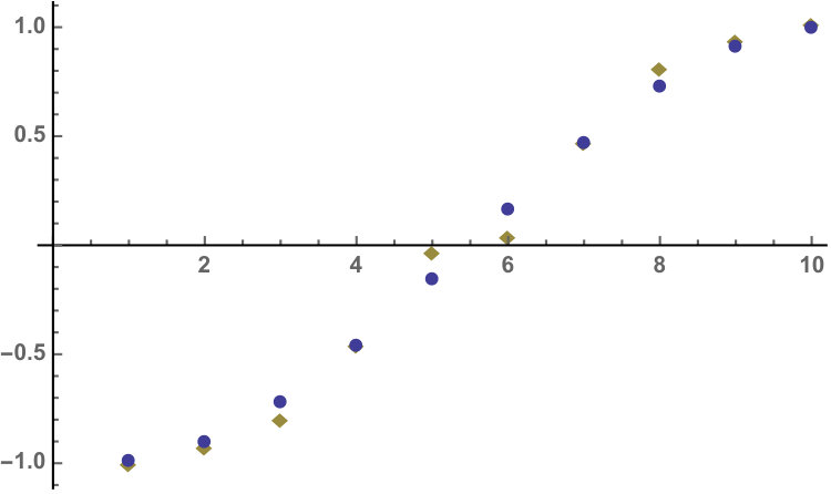 Figure 14
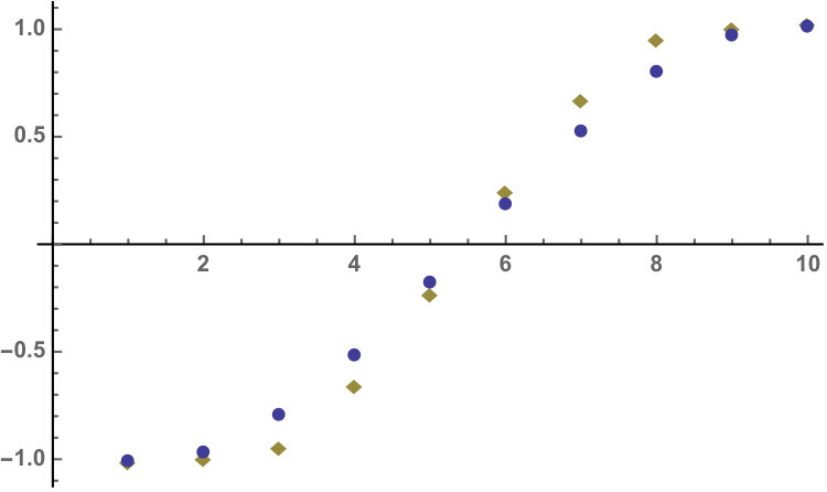 Figure 15
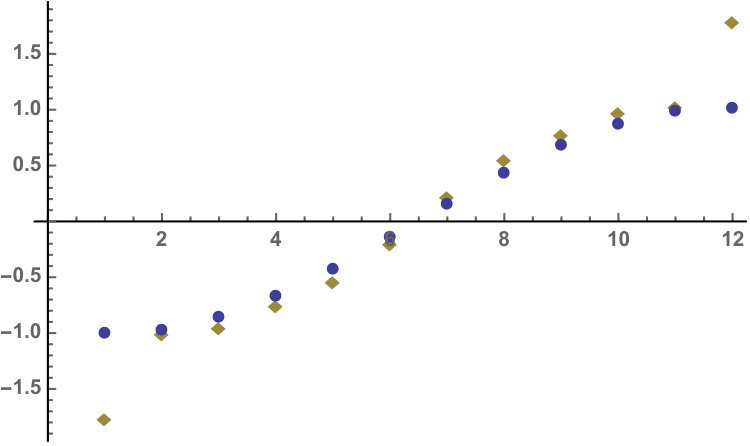 Figure 16
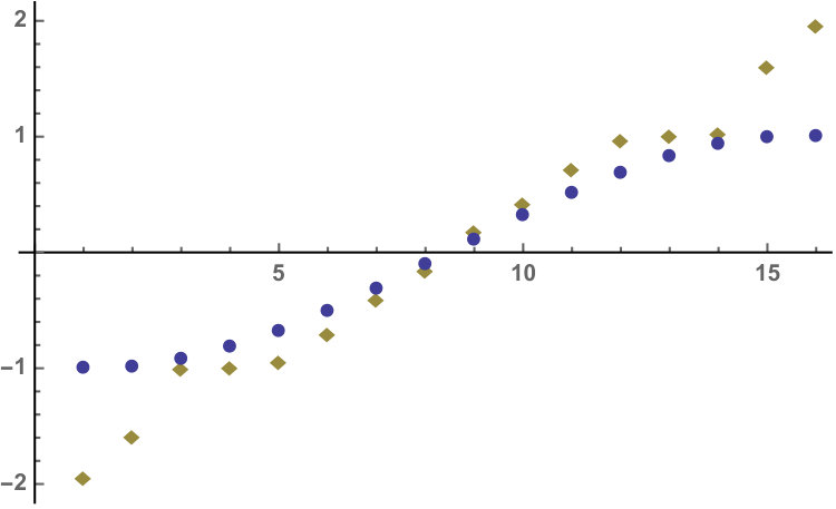 Figure 17
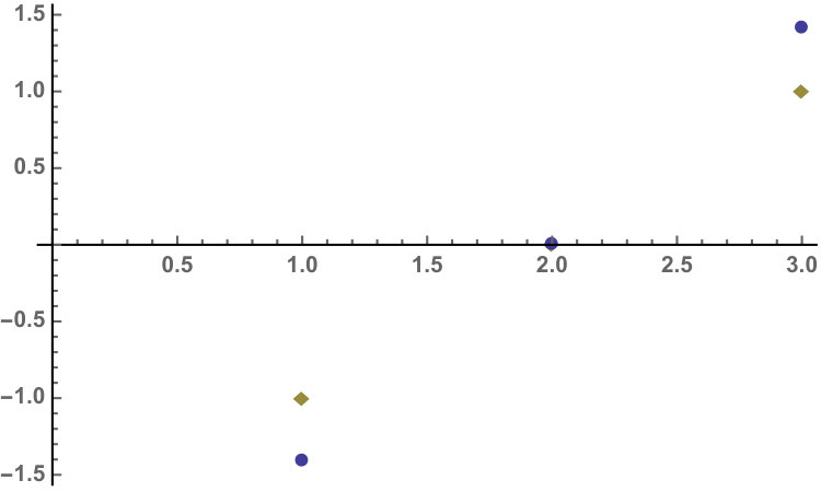 Figure 18
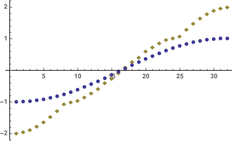 Figure 19
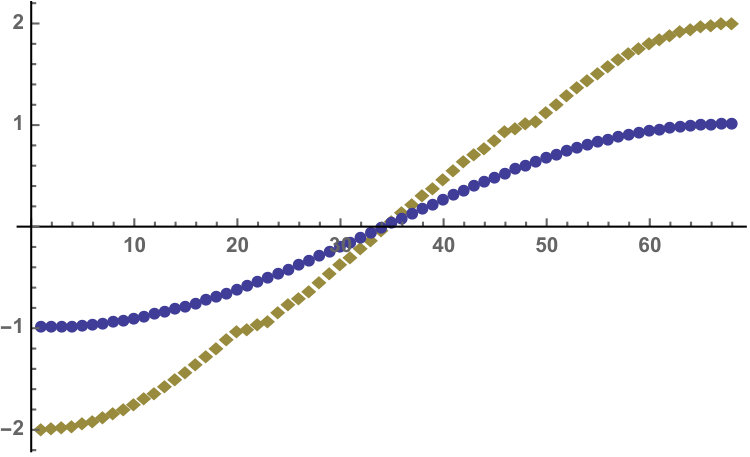 Figure 20
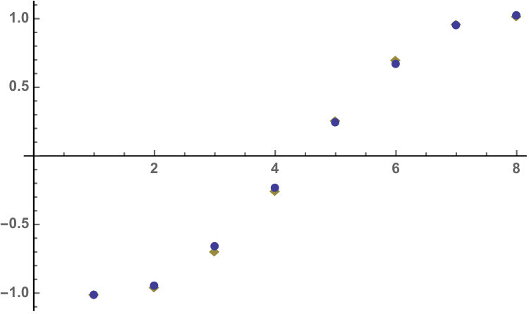 Figure 21
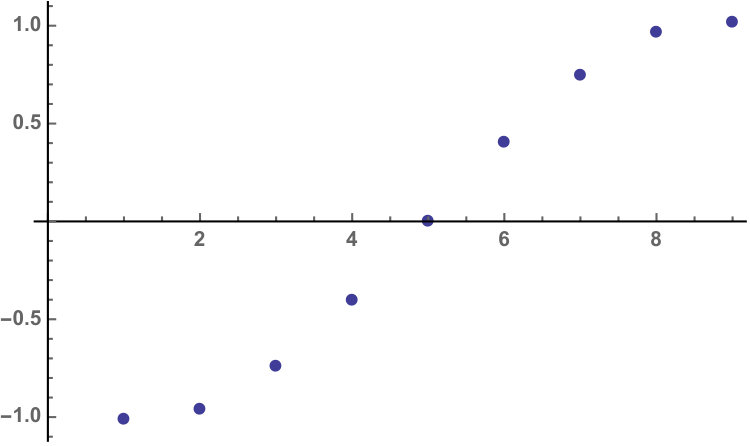 Figure 22
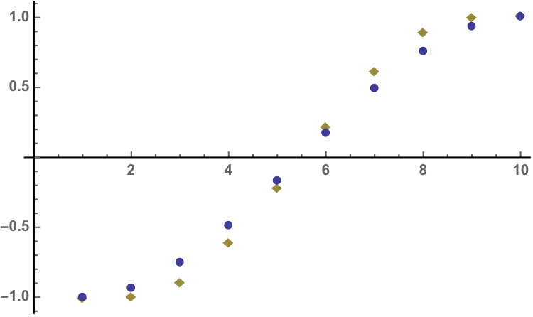 Figure 23
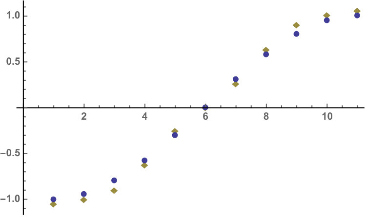 Figure 24
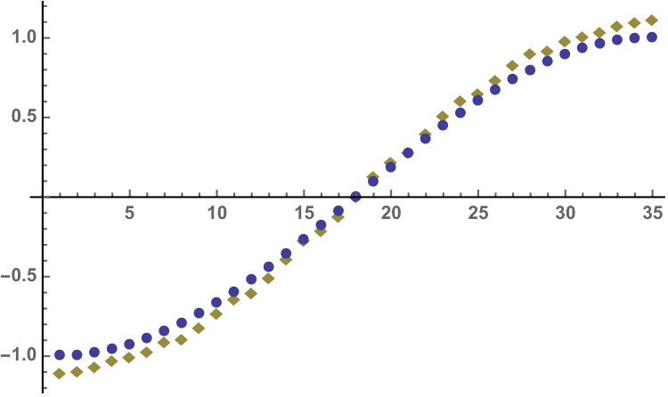 Figure 25
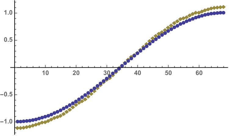 Figure 26
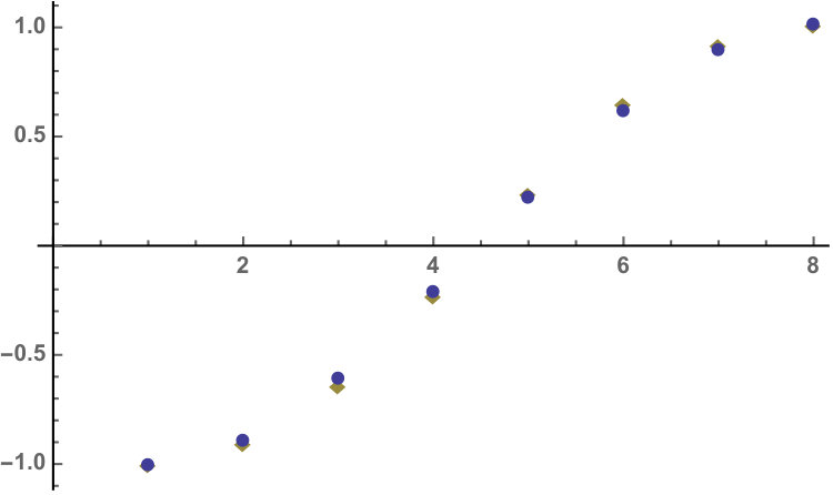 Figure 27
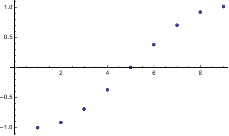 Figure 28
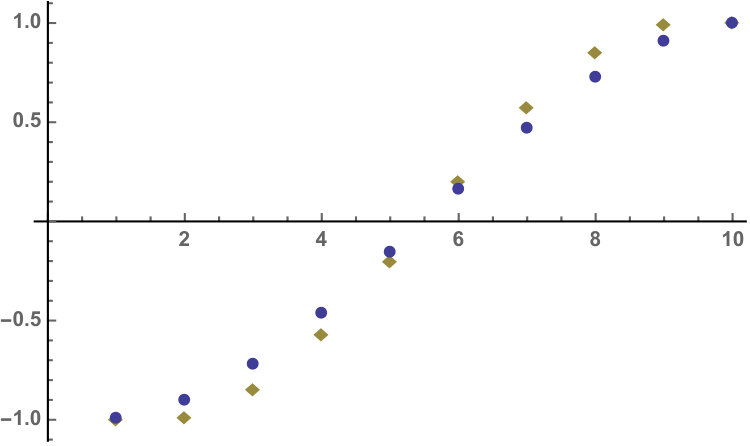 Figure 29
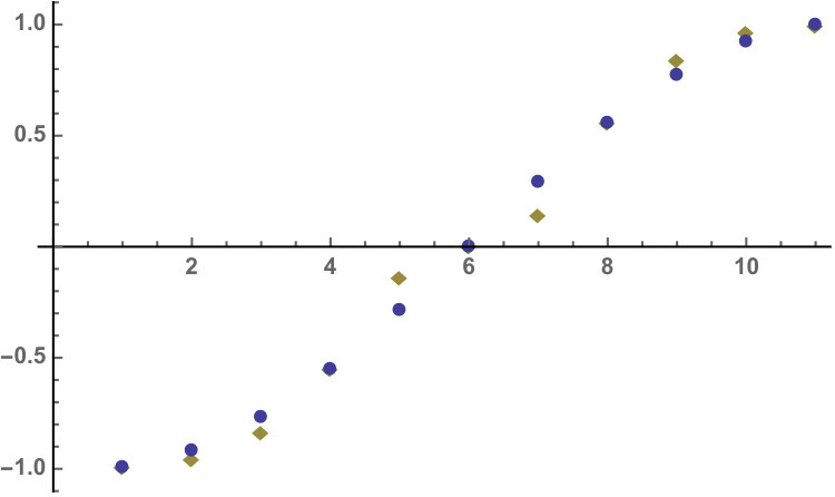 Figure 30
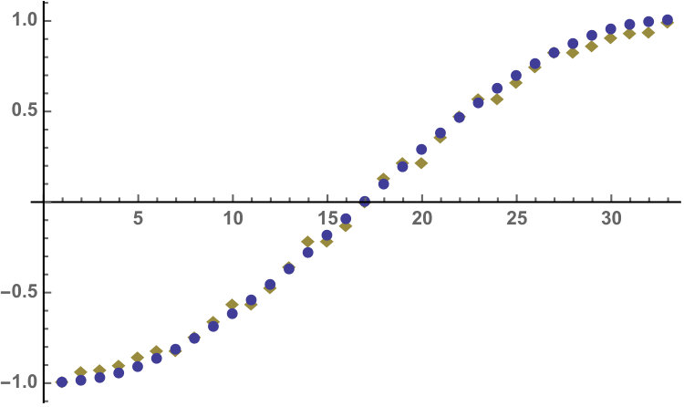 Figure 31
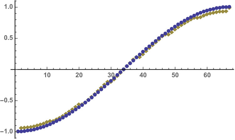 Figure 32
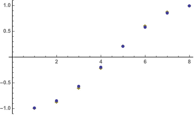 Figure 33
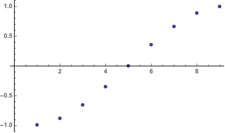 Figure 34
Peer Reviews
No public reviews on file for this paper yet. If you reviewed it on a platform where reviews are public (OpenReview, ICLR, NeurIPS, ICML), you can paste yours below so the community can read it here.
Videos
No videos yet. Explain this paper in a talk, walkthrough, or lecture? Add one.
Orthogonal sequences constructed from quasi-orthogonal ultraspherical polynomials
Oksana Bihun*†111Corresponding author: [email protected]. and Kathy Driver‡*
*†*Department of Mathematics, University of Colorado, Colorado Springs
1420 Austin Bluffs Pkwy, Colorado Springs, CO 80918, USA
*‡*Department of Mathematics and Applied Mathematics, University of Cape Town,
Private Bag X3, Rondebosch 7701, South Africa
Abstract
Let and , be two sets of real, distinct points satisfying the interlacing property In [10], Wendroff proved that if and , then and can be embedded in a non-unique monic orthogonal sequence We investigate a question raised by Mourad Ismail at OPSFA 2015 as to the nature and properties of orthogonal sequences generated by applying Wendroff’s Theorem to the interlacing zeros of and , where is a sequence of monic ultraspherical polynomials and We construct an algorithm for generating infinite monic orthogonal sequences from the two polynomials and , which is applicable for each pair of fixed parameters in the ranges and , . We plot and compare the zeros of and for several choices of and a range of values of the parameters and . For the curves that the zeros of and approach are substantially different for large values of When the two curves have a similar shape while the curves are almost identical for
MSC: primary 33C50; secondary 42C05.
Keywords: Ultraspherical polynomials, Wendroff’s Theorem, interlacing of zeros, quasi-orthogonal polynomials.
1 Introduction
The monic ultraspherical polynomial is defined by the three term recurrence relation [8, eqn.(8.18)]
[TABLE]
where
[TABLE]
For each the sequence is orthogonal on with respect to the weight function and for each the zeros of are real, simple, symmetric, lie in and the zeros of interlace with the zeros of ( see [9, Theorem 3.3.2]) namely,
[TABLE]
where are the zeros of in increasing order.
As decreases below two (symmetric) zeros of leave the interval through the endpoints and ( see [5, p. 296] ) and remain real with absolute value for each and For the sequence is quasi-orthogonal of order with respect to the weight function , (see [2, Theorem 6] and [3, p.144]) and, for any ( see [6, Theorem 3.1]),
[TABLE]
It follows from that the zeros of and are not interlacing for any and but we see from and that the zeros of interlace with the zeros of for each and each with
In 1961, Wendroff [10, p. 554] proved that, for any fixed positive integer if and are two sets of real, distinct points satisfying the interlacing property there exist infinitely many sequences of monic orthogonal polynomials with and His proof is constructive and for a given, fixed each polynomial of degree is uniquely determined by and In contrast, the monic polynomials of degree in any orthogonal sequence that includes and are only constrained by the requirement that any infinite sequence of (monic) orthogonal polynomials satisfies a three term recurrence relation of the form
[TABLE]
Since there are infinitely many choices of the coefficients and with and for there are infinitely many distinct monic orthogonal sequences that include and
Here, we fix , fix , , and define
[TABLE]
We investigate the properties of the zeros of polynomials in monic orthogonal sequences generated by the Wendroff process. It is important to emphasize the dependence on the “starting value” of when generating each monic orthogonal sequence that includes and If is large, the number of polynomials (namely, ) that are uniquely determined in every monic orthogonal sequence that includes and is correspondingly large whereas, for example, if we have two degrees of freedom when generating each of the monic polynomials of degree and exactly of the polynomials of lower degree are completely determined. The restriction arises from the fact that when the quadratic ultraspherical polynomial has two pure imaginary zeros (see [3, p. 144]). If we restrict to the range the results proved here apply for
2 Notation
For each denote
[TABLE]
[TABLE]
The zeros of are distinct, real and symmetric with respect to the origin for so that for all while the zeros of are distinct, real and symmetric when or so that Note that
[TABLE]
and
[TABLE]
3 Orthogonal sequences generated by and
Our main result is the following theorem.
Theorem 3.1
Let be the sequence of monic ultraspherical polynomials defined by and Fix fix and suppose that is abitrary.
Define
[TABLE]
where is the largest zero of
Let the sequence of monic polynomials be defined by:
[TABLE]
where
[TABLE]
and is the coefficient of in , see (8). Then the sequence is symmetric and orthogonal with respect to a positive measure supported on the interval .
Proof of Theorem 3.1
Fix The monic polynomial is uniquely determined by
[TABLE]
where and are defined by and the coefficient is chosen so that is monic. The positivity of follows from the interlacing property of the zeros of and In the same way, for each , the polynomial is constructed from the polynomials and The process is repeated until we obtain The polynomials are constructed recursively using the three-term recurrence relation
[TABLE]
choosing positive coefficients for This ensures (Favard’s Theorem) that the infinite sequence is orthogonal with respect to a positive measure. Wendroff mentions in his proof [10, p. 554] that the coefficients can be chosen in such a way that all zeros of lie in the interval for each but does not indicate how to choose the coefficients to achieve this outcome. Here, we prove that the choice of given in ensures that all the zeros of lie in the interval Applying the same argument iteratively, it can be shown that the choice of given in ensures that the zeros of lie in the interval for each
Suppose We show that the zeros of lie in the interval . From with replaced by it follows immediately that the zeros of and lie in the open interval In addition, and are monic polynomials with no zeros greater than so and Since it follows that . By construction, the zeros of and interlace and the zeros of lie in the interval so it follows that and We need to show that the largest zero of satisfies .
From with we have so that
[TABLE]
On the other hand, since we are assuming that we have
[TABLE]
Therefore, and so that as required.
Remark 3.1. The sequences of polynomials defined in Theorem 3.1 with and are (by construction) orthogonal for each and satisfying . It is therefore natural to compare orthogonal sequences generated by the Wendroff process with the sequences of ultraspherical polynomials orthogonal on . In this case, we can choose so the interval contains the zeros of all the polynomials in the sequence as well as the sequence .
Remark 3.2. For and fixed, the largest (real) zero of is bounded above by see [7, (4)]. An alternative upper bound for is given by
see [7, (15)]. These bounds give estimates for the interval of orthogonality of the sequences , where and .
Remark 3.3. For and fixed, we can choose in Theorem 3.1 in such a way that the interval contains all the zeros of the polynomials . To this end, we use the estimates and , , see [7], where is the largest zero of . Because and , we may choose independent of , namely
[TABLE]
or
[TABLE]
To choose the sharper of the two bounds and , we use the following comparisons: , if and if . Note that and for .
Remark 3.4. When developing an algorithm for generating orthogonal sequences, we can choose , , where . Using this expression for and putting into (14), we obtain for all . The advantage of choosing , , with , is that all coefficients are equal, namely, for . This results in a significant reduction in the computational complexity of the algorithm.
4 Algorithm for construction of fixed, ,
Using Theorem 3.1 and Remarks 1,3,4, we present an algorithm for construction of the first terms of orthogonal sequences .
Choose integers and . 2. 2.
Choose with , 3. 3.
If , define . If , define . If , define . 4. 4.
Choose . 5. 5.
Let . 6. 6.
For , let be the coefficient of in . 7. 7.
For ,
let ;
let ;
let be the coefficient of in . 8. 8.
Let and . 9. 9.
For , let .
The above algorithm generates the first terms of a sequence of symmetric polynomials orthogonal with respect to some positive measure supported on the interval , which contains all the zeros of the symmetric polynomials . If and , the sequence is quasi-orthogonal of order on with respect to the weight function ; if and , for , the sequence is orthogonal with respect to the weight function on the interval .
Example 4.1. In this example we present the first 11 terms of the sequence using our algorithm with , , , and , where , and , :
[TABLE]
5 The zeros of and
In this section, we plot and compare the zeros of constructed using the algorithm in Section 4 with the zeros of , where and , are fixed integers.
Example 5.1. Let and Choose , and The polynomials are listed below with the approximate values of their zeros in curly brackets :
[TABLE]
Note that the zeros of are The largest and smallest zeros of are close to the limits and
In Figures 1 through 4, the -coordinates of the plotted points are the zeros of (diamond, brown) and (round, blue) for . The figures suggest that the greatest difference between the zeros of and are at the extreme zeros.
Example 5.1 provides numerical confirmation that the relative ordering of the zeros of and , is consistent with [1, Theorem 4]. Replacing by and putting in (7) and (8) in [1, Theorem 4], the negative zeros of should satisfy
[TABLE]
while the positive zeros of should satisfy
[TABLE]
From Example 5.1, we see that the zeros of , , and satisfy
[TABLE]
and
[TABLE]
as expected.
In the examples and figures that follow, we plot the zeros of and for selected values of (the “starting value” ), and
Example 5.2. Let , , and , as in the previous example. In Figures 5 and 6, the -coordinates of the plotted points are the zeros of (diamond, brown) and (round, blue) respectively for , and , .
Example 5.3. Let , , Choose and . In Figures 7 through 14 the -coordinates of the plotted points are the zeros of (diamond, brown) and (round, blue) for selected integer values of between and . The figures suggest that, as increases, the curves that fit the zeros of and are significantly different.
Example 5.4. Let , , Choose and . In Figures 15 through 20 the -coordinates of the plotted points are the zeros of and for selected integer values of between and .
Example 5.5. Let , , Choose and . In Figures 21 through 26 the -coordinates of the plotted points are the zeros of and for several integer values of between and .
Remark 5.2. As increases, the zeros of and appear to be asymptotically equal for . This is not unexpected since lies in the orthogonal range for ultraspherical polynomials. Note that the interval of orthogonality is , where
Example 5.6. Let , , In Figures 27 through 34, the -coordinates of the plotted points are the zeros of and for a selection of values of with , where is fixed. We choose if and if ; the zeros of and are contained in .
For the curves to which the zeros of and can be fitted are substantially different for some values of As approaches from the left, the two curves are very similar, and, as increases further, the curves are almost identical.
6 Acknowledgements
Kathy Driver would like to express her thanks to the Mathematics Department, University of Colorado, Colorado Springs, for its hospitality during her visit in Spring 2018, during which the work on this paper began.
7 Bibliography
The reference list from the paper itself. Each links out to its DOI / PubMed record.
- 1[1] Beardon, A., Driver, K., Jordaan, K. Zeros of polynomials embedded in an orthogonal sequence, Numer. Algor. 48 (3) (2011) 399–403.
- 2[2] Brezinski, C., Driver, K. A., and Redivo-Zaglia, M. Quasi-orthogonality with applications to some families of classical orthogonal polynomials, Applied Numerical Mathematics, 48 (2004) 157–168.
- 3[3] Brezinski, C., Driver, K. A., and Redivo-Zaglia, M. Zeros of quadratic quasi-orthogonal order 2 polynomials, Applied Numerical Mathematics, 139 (2019) 143–145.
- 4[4] Chihara, T.S. On quasi–orthogonal polynomials, Proc. Amer. Math. Soc. 8 (1957) 765–767.
- 5[5] Driver, K., Duren , P. Zeros of ultraspherical polynomials and the Hilbert-Klein formulas , J. Comp. Appl. Math. 135 (2001) 293–301.
- 6[6] Driver, K., Muldoon, M. E. Zeros of quasi-orthogonal ultraspherical polynomials, Indag. Math. 27(4) (2016) 930–944.
- 7[7] Driver, K., Muldoon, M. E. Bounds for extreme zeros of quasi-orthogonal ultraspherical polynomials, J. Class. Anal. 9 (2016) 69–78.
- 8[8] Koekoek, R., Lesky, P. A., Swarttouw, R. F., Hypergeometric Orthogonal Polynomials and their q-Analogues, Springer Monographs in Mathematics (2010).