Direct Measurement of the Cosmic-Ray Proton Spectrum from 50 GeV to 10 TeV with the Calorimetric Electron Telescope on the International Space Station
O. Adriani, Y. Akaike, K. Asano, Y. Asaoka, M.G. Bagliesi, E. Berti,, G. Bigongiari, W.R. Binns, S. Bonechi, M. Bongi, A. Bruno, J.H. Buckley, N., Cannady, G. Castellini, C. Checchia, M.L. Cherry, G. Collazuol, V. Di Felice,, K. Ebisawa, H. Fuke, T.G. Guzik, T. Hams, N. Hasebe

TL;DR
This paper reports the first space-based measurement of the cosmic-ray proton spectrum from 50 GeV to 10 TeV using CALET on the ISS, confirming spectral hardening and extending previous measurements to higher energies.
Contribution
It provides a continuous measurement of the cosmic-ray proton spectrum over a wide energy range with a single instrument, bridging gaps between prior separate subrange studies.
Findings
Spectrum consistent with AMS-02 at overlapping energies
Extended measurement up to 10 TeV, nearly an order of magnitude higher
Confirmed spectral hardening and deviation from single power law
Abstract
In this paper, we present the analysis and results of a direct measurement of the cosmic-ray proton spectrum with the CALET instrument onboard the International Space Station, including the detailed assessment of systematic uncertainties. The observation period used in this analysis is from October 13, 2015 to August 31, 2018 (1054 days). We have achieved the very wide energy range necessary to carry out measurements of the spectrum from 50 GeV to 10 TeV covering, for the first time in space, with a single instrument the whole energy interval previously investigated in most cases in separate subranges by magnetic spectrometers (BESS-TeV, PAMELA, and AMS-02) and calorimetric instruments (ATIC, CREAM, and NUCLEON). The observed spectrum is consistent with AMS-02 but extends to nearly an order of magnitude higher energy, showing a very smooth transition of the power-law spectral index from…
Click any figure to enlarge with its caption.
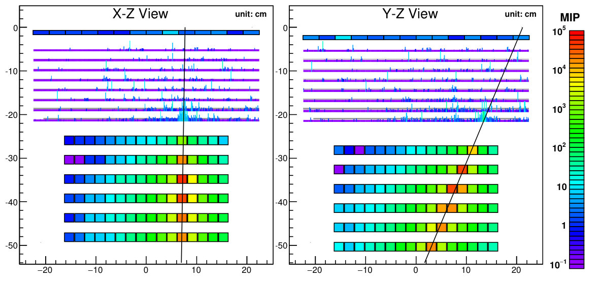 Figure 1
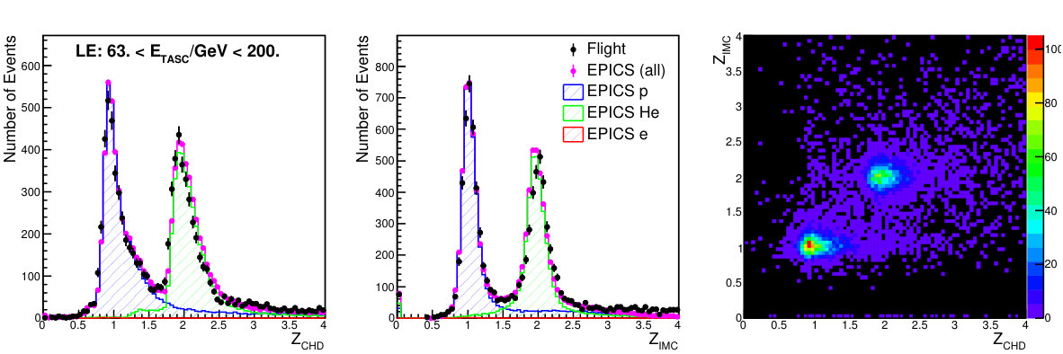 Figure 2
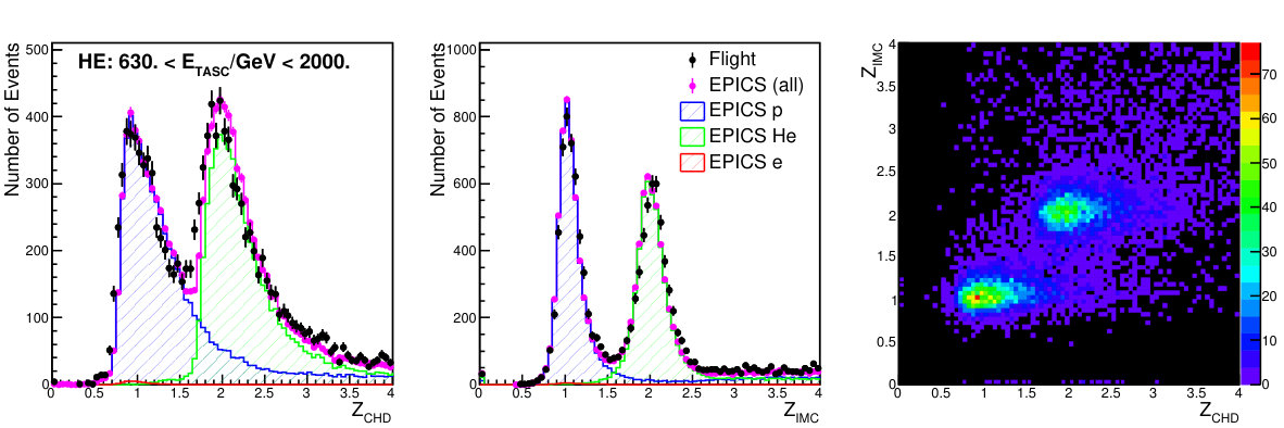 Figure 3
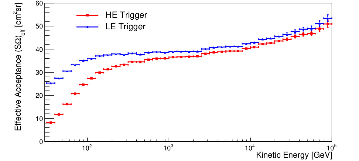 Figure 4
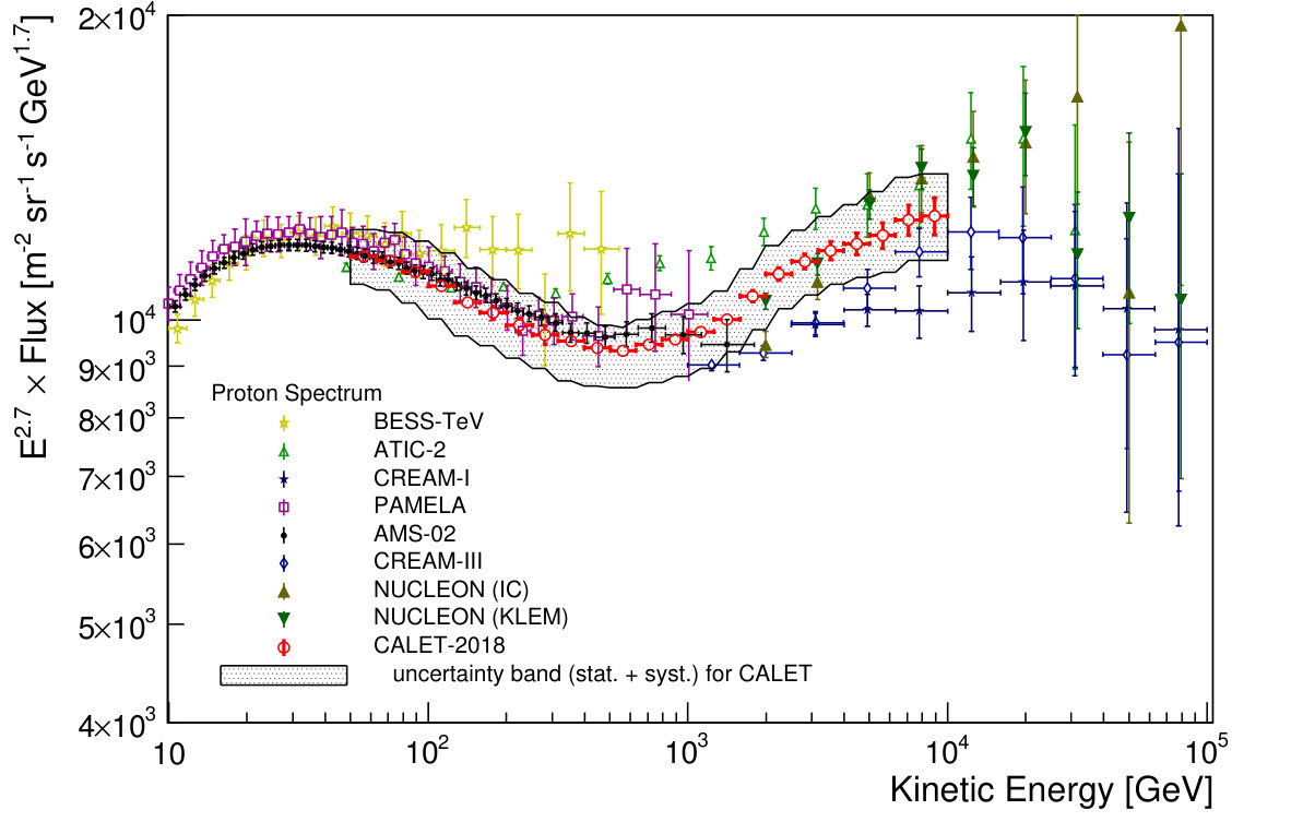 Figure 5
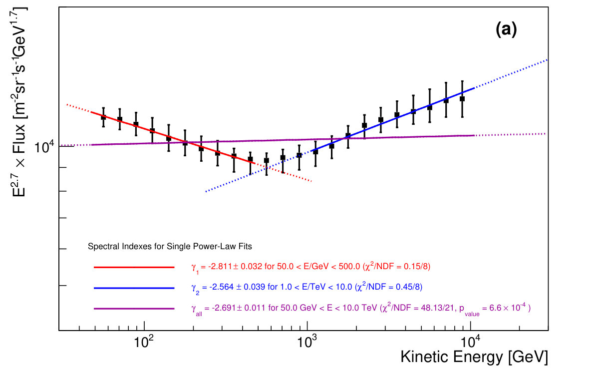 Figure 6
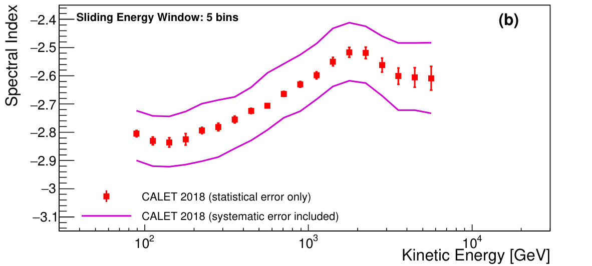 Figure 7
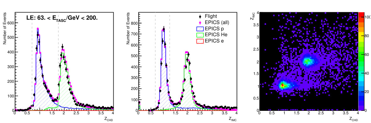 Figure 8
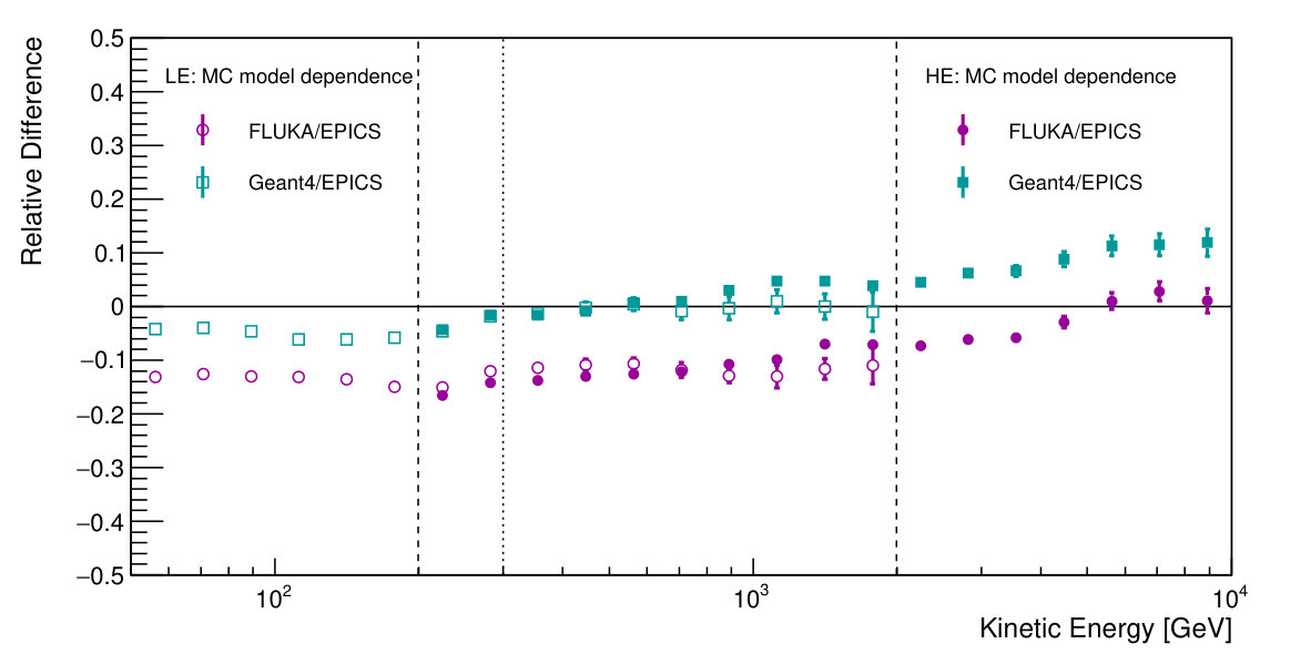 Figure 9
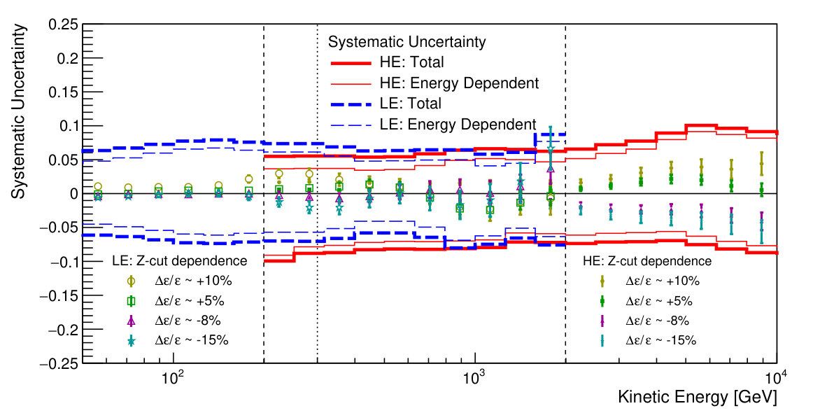 Figure 10
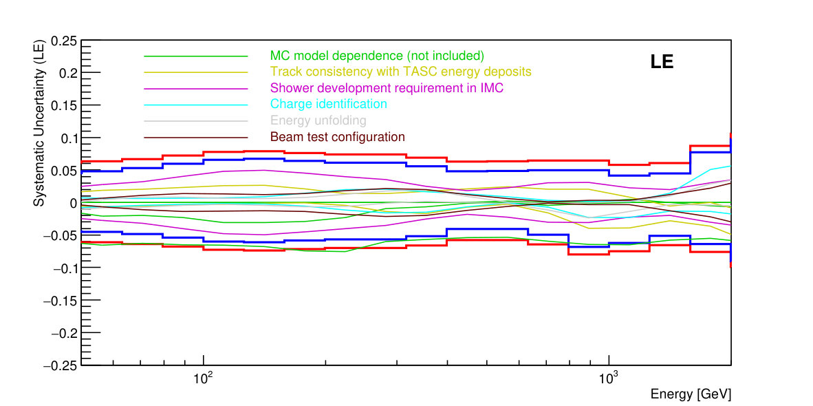 Figure 11
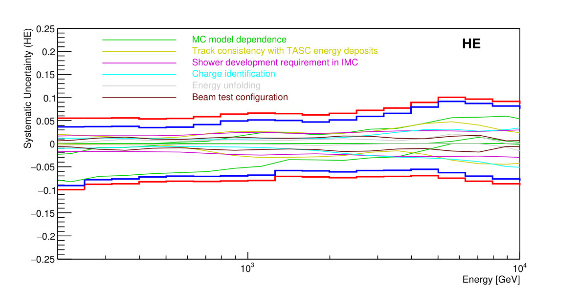 Figure 12
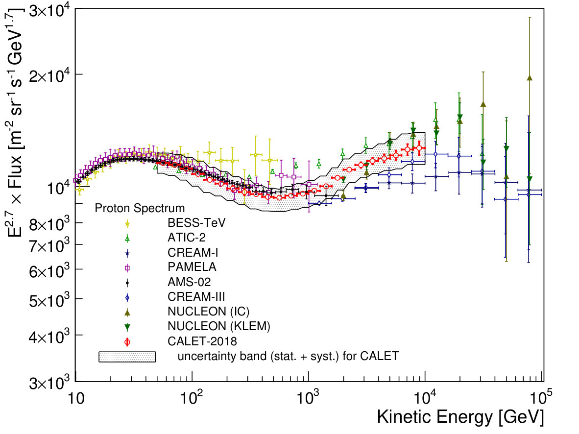 Figure 13
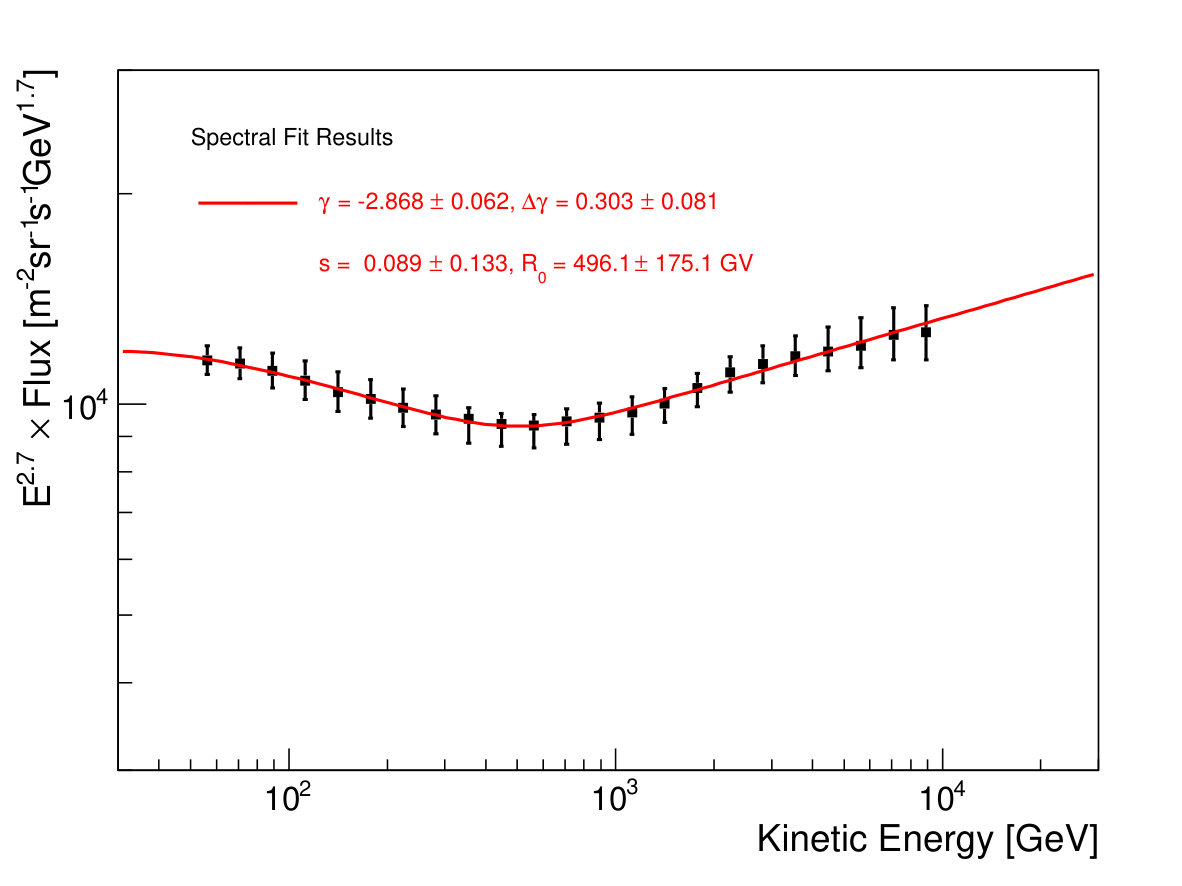 Figure 14
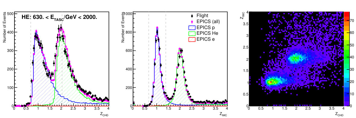 Figure 15
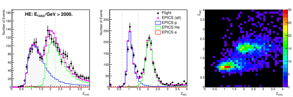 Figure 16
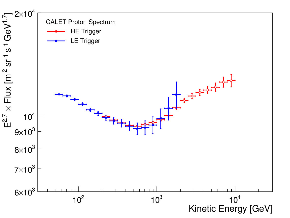 Figure 17
| Energy Bin | Representative Energy | Flux |
|---|---|---|
| (GeV) | (GeV) | (m-2sr-1s-1GeV-1) |
| 50.1–63.1 | ||
| 63.1–79.4 | ||
| 79.4–100.0 | ||
| 100.0–125.9 | ||
| 125.9–158.5 | ||
| 158.5–199.5 | ||
| 199.5–251.2 | ||
| 251.2–316.2 | ||
| 316.2–398.1 | ||
| 398.1–501.2 | ||
| 501.2–631.0 | ||
| 631.0–794.3 | ||
| 794.3–1000.0 | ||
| 1000.0–1258.9 | ||
| 1258.9–1584.9 | ||
| 1584.9–1995.3 | ||
| 1995.3–2511.9 | ||
| 2511.9–3162.3 | ||
| 3162.3–3981.1 | ||
| 3981.1–5011.9 | ||
| 5011.9–6309.6 | ||
| 6309.6–7943.3 | ||
| 7943.3–10000.0 |
Peer Reviews
No public reviews on file for this paper yet. If you reviewed it on a platform where reviews are public (OpenReview, ICLR, NeurIPS, ICML), you can paste yours below so the community can read it here.
Videos
No videos yet. Explain this paper in a talk, walkthrough, or lecture? Add one.
CALET Collaboration
Direct Measurement of the Cosmic-Ray Proton Spectrum
from 50 GeV to 10 TeV with the Calorimetric Electron Telescope
on the International Space Station
O. Adriani
Department of Physics, University of Florence, Via Sansone, 1 - 50019 Sesto, Fiorentino, Italy
INFN Sezione di Florence, Via Sansone, 1 - 50019 Sesto, Fiorentino, Italy
Y. Akaike
Department of Physics, University of Maryland, Baltimore County, 1000 Hilltop Circle, Baltimore, Maryland 21250, USA
Astroparticle Physics Laboratory, NASA/GSFC, Greenbelt, Maryland 20771, USA
K. Asano
Institute for Cosmic Ray Research, The University of Tokyo, 5-1-5 Kashiwa-no-Ha, Kashiwa, Chiba 277-8582, Japan
Y. Asaoka
Waseda Research Institute for Science and Engineering, Waseda University, 3-4-1 Okubo, Shinjuku, Tokyo 169-8555, Japan
JEM Utilization Center, Human Spaceflight Technology Directorate, Japan Aerospace Exploration Agency, 2-1-1 Sengen, Tsukuba, Ibaraki 305-8505, Japan
M.G. Bagliesi
Department of Physical Sciences, Earth and Environment, University of Siena, via Roma 56, 53100 Siena, Italy
INFN Sezione di Pisa, Polo Fibonacci, Largo B. Pontecorvo, 3 - 56127 Pisa, Italy
E. Berti
Department of Physics, University of Florence, Via Sansone, 1 - 50019 Sesto, Fiorentino, Italy
INFN Sezione di Florence, Via Sansone, 1 - 50019 Sesto, Fiorentino, Italy
G. Bigongiari
Department of Physical Sciences, Earth and Environment, University of Siena, via Roma 56, 53100 Siena, Italy
INFN Sezione di Pisa, Polo Fibonacci, Largo B. Pontecorvo, 3 - 56127 Pisa, Italy
W.R. Binns
Department of Physics and McDonnell Center for the Space Sciences, Washington University, One Brookings Drive, St. Louis, Missouri 63130-4899, USA
S. Bonechi
Department of Physical Sciences, Earth and Environment, University of Siena, via Roma 56, 53100 Siena, Italy
INFN Sezione di Pisa, Polo Fibonacci, Largo B. Pontecorvo, 3 - 56127 Pisa, Italy
M. Bongi
Department of Physics, University of Florence, Via Sansone, 1 - 50019 Sesto, Fiorentino, Italy
INFN Sezione di Florence, Via Sansone, 1 - 50019 Sesto, Fiorentino, Italy
A. Bruno
Heliospheric Physics Laboratory, NASA/GSFC, Greenbelt, Maryland 20771, USA
J.H. Buckley
Department of Physics and McDonnell Center for the Space Sciences, Washington University, One Brookings Drive, St. Louis, Missouri 63130-4899, USA
N. Cannady
Department of Physics and Astronomy, Louisiana State University, 202 Nicholson Hall, Baton Rouge, Louisiana 70803, USA
G. Castellini
Institute of Applied Physics (IFAC), National Research Council (CNR), Via Madonna del Piano, 10, 50019 Sesto, Fiorentino, Italy
C. Checchia
Department of Physics and Astronomy, University of Padova, Via Marzolo, 8, 35131 Padova, Italy
INFN Sezione di Padova, Via Marzolo, 8, 35131 Padova, Italy
M.L. Cherry
Department of Physics and Astronomy, Louisiana State University, 202 Nicholson Hall, Baton Rouge, Louisiana 70803, USA
G. Collazuol
Department of Physics and Astronomy, University of Padova, Via Marzolo, 8, 35131 Padova, Italy
INFN Sezione di Padova, Via Marzolo, 8, 35131 Padova, Italy
V. Di Felice
University of Rome “Tor Vergata”, Via della Ricerca Scientifica 1, 00133 Rome, Italy
INFN Sezione di Rome “Tor Vergata”, Via della Ricerca Scientifica 1, 00133 Rome, Italy
K. Ebisawa
Institute of Space and Astronautical Science, Japan Aerospace Exploration Agency, 3-1-1 Yoshinodai, Chuo, Sagamihara, Kanagawa 252-5210, Japan
H. Fuke
Institute of Space and Astronautical Science, Japan Aerospace Exploration Agency, 3-1-1 Yoshinodai, Chuo, Sagamihara, Kanagawa 252-5210, Japan
T.G. Guzik
Department of Physics and Astronomy, Louisiana State University, 202 Nicholson Hall, Baton Rouge, Louisiana 70803, USA
T. Hams
Department of Physics, University of Maryland, Baltimore County, 1000 Hilltop Circle, Baltimore, Maryland 21250, USA
CRESST and Astroparticle Physics Laboratory NASA/GSFC, Greenbelt, Maryland 20771, USA
N. Hasebe
Waseda Research Institute for Science and Engineering, Waseda University, 3-4-1 Okubo, Shinjuku, Tokyo 169-8555, Japan
K. Hibino
Kanagawa University, 3-27-1 Rokkakubashi, Kanagawa, Yokohama, Kanagawa 221-8686, Japan
M. Ichimura
Faculty of Science and Technology, Graduate School of Science and Technology, Hirosaki University, 3, Bunkyo, Hirosaki, Aomori 036-8561, Japan
K. Ioka
Yukawa Institute for Theoretical Physics, Kyoto University, Kitashirakawa Oiwakecho, Sakyo, Kyoto 606-8502, Japan
W. Ishizaki
Institute for Cosmic Ray Research, The University of Tokyo, 5-1-5 Kashiwa-no-Ha, Kashiwa, Chiba 277-8582, Japan
M.H. Israel
Department of Physics and McDonnell Center for the Space Sciences, Washington University, One Brookings Drive, St. Louis, Missouri 63130-4899, USA
K. Kasahara
Waseda Research Institute for Science and Engineering, Waseda University, 3-4-1 Okubo, Shinjuku, Tokyo 169-8555, Japan
J. Kataoka
Waseda Research Institute for Science and Engineering, Waseda University, 3-4-1 Okubo, Shinjuku, Tokyo 169-8555, Japan
R. Kataoka
National Institute of Polar Research, 10-3, Midori-cho, Tachikawa, Tokyo 190-8518, Japan
Y. Katayose
Faculty of Engineering, Division of Intelligent Systems Engineering, Yokohama National University, 79-5 Tokiwadai, Hodogaya, Yokohama 240-8501, Japan
C. Kato
Faculty of Science, Shinshu University, 3-1-1 Asahi, Matsumoto, Nagano 390-8621, Japan
N. Kawanaka
Hakubi Center, Kyoto University, Yoshida Honmachi, Sakyo-ku, Kyoto 606-8501, Japan
Department of Astronomy, Graduate School of Science, Kyoto University, Kitashirakawa Oiwake-cho, Sakyo-ku, Kyoto 606-8502, Japan
Y. Kawakubo
Department of Physics and Astronomy, Louisiana State University, 202 Nicholson Hall, Baton Rouge, Louisiana 70803, USA
College of Science and Engineering, Department of Physics and Mathematics, Aoyama Gakuin University, 5-10-1 Fuchinobe, Chuo, Sagamihara, Kanagawa 252-5258, Japan
K. Kohri
Institute of Particle and Nuclear Studies, High Energy Accelerator Research Organization, 1-1 Oho, Tsukuba, Ibaraki 305-0801, Japan
H.S. Krawczynski
Department of Physics and McDonnell Center for the Space Sciences, Washington University, One Brookings Drive, St. Louis, Missouri 63130-4899, USA
J.F. Krizmanic
CRESST and Astroparticle Physics Laboratory NASA/GSFC, Greenbelt, Maryland 20771, USA
Department of Physics, University of Maryland, Baltimore County, 1000 Hilltop Circle, Baltimore, Maryland 21250, USA
T. Lomtadze
INFN Sezione di Pisa, Polo Fibonacci, Largo B. Pontecorvo, 3 - 56127 Pisa, Italy
P. Maestro
Department of Physical Sciences, Earth and Environment, University of Siena, via Roma 56, 53100 Siena, Italy
INFN Sezione di Pisa, Polo Fibonacci, Largo B. Pontecorvo, 3 - 56127 Pisa, Italy
P.S. Marrocchesi
Department of Physical Sciences, Earth and Environment, University of Siena, via Roma 56, 53100 Siena, Italy
INFN Sezione di Pisa, Polo Fibonacci, Largo B. Pontecorvo, 3 - 56127 Pisa, Italy
A.M. Messineo
University of Pisa, Polo Fibonacci, Largo B. Pontecorvo, 3 - 56127 Pisa, Italy
INFN Sezione di Pisa, Polo Fibonacci, Largo B. Pontecorvo, 3 - 56127 Pisa, Italy
J.W. Mitchell
Astroparticle Physics Laboratory, NASA/GSFC, Greenbelt, Maryland 20771, USA
S. Miyake
Department of Electrical and Electronic Systems Engineering, National Institute of Technology, Ibaraki College, 866 Nakane, Hitachinaka, Ibaraki 312-8508 Japan
A.A. Moiseev
Department of Astronomy, University of Maryland, College Park, Maryland 20742, USA
CRESST and Astroparticle Physics Laboratory NASA/GSFC, Greenbelt, Maryland 20771, USA
K. Mori
Waseda Research Institute for Science and Engineering, Waseda University, 3-4-1 Okubo, Shinjuku, Tokyo 169-8555, Japan
Institute of Space and Astronautical Science, Japan Aerospace Exploration Agency, 3-1-1 Yoshinodai, Chuo, Sagamihara, Kanagawa 252-5210, Japan
M. Mori
Department of Physical Sciences, College of Science and Engineering, Ritsumeikan University, Shiga 525-8577, Japan
N. Mori
INFN Sezione di Florence, Via Sansone, 1 - 50019 Sesto, Fiorentino, Italy
H.M. Motz
Faculty of Science and Engineering, Global Center for Science and Engineering, Waseda University, 3-4-1 Okubo, Shinjuku, Tokyo 169-8555, Japan
K. Munakata
Faculty of Science, Shinshu University, 3-1-1 Asahi, Matsumoto, Nagano 390-8621, Japan
H. Murakami
Waseda Research Institute for Science and Engineering, Waseda University, 3-4-1 Okubo, Shinjuku, Tokyo 169-8555, Japan
S. Nakahira
RIKEN, 2-1 Hirosawa, Wako, Saitama 351-0198, Japan
J. Nishimura
Institute of Space and Astronautical Science, Japan Aerospace Exploration Agency, 3-1-1 Yoshinodai, Chuo, Sagamihara, Kanagawa 252-5210, Japan
G.A. de Nolfo
Heliospheric Physics Laboratory, NASA/GSFC, Greenbelt, Maryland 20771, USA
S. Okuno
Kanagawa University, 3-27-1 Rokkakubashi, Kanagawa, Yokohama, Kanagawa 221-8686, Japan
J.F. Ormes
Department of Physics and Astronomy, University of Denver, Physics Building, Room 211, 2112 East Wesley Avenue, Denver, Colorado 80208-6900, USA
S. Ozawa
Waseda Research Institute for Science and Engineering, Waseda University, 3-4-1 Okubo, Shinjuku, Tokyo 169-8555, Japan
L. Pacini
Department of Physics, University of Florence, Via Sansone, 1 - 50019 Sesto, Fiorentino, Italy
Institute of Applied Physics (IFAC), National Research Council (CNR), Via Madonna del Piano, 10, 50019 Sesto, Fiorentino, Italy
INFN Sezione di Florence, Via Sansone, 1 - 50019 Sesto, Fiorentino, Italy
F. Palma
University of Rome “Tor Vergata”, Via della Ricerca Scientifica 1, 00133 Rome, Italy
INFN Sezione di Rome “Tor Vergata”, Via della Ricerca Scientifica 1, 00133 Rome, Italy
P. Papini
INFN Sezione di Florence, Via Sansone, 1 - 50019 Sesto, Fiorentino, Italy
A.V. Penacchioni
Department of Physical Sciences, Earth and Environment, University of Siena, via Roma 56, 53100 Siena, Italy
ASI Science Data Center (ASDC), Via del Politecnico snc, 00133 Rome, Italy
B.F. Rauch
Department of Physics and McDonnell Center for the Space Sciences, Washington University, One Brookings Drive, St. Louis, Missouri 63130-4899, USA
S.B. Ricciarini
Institute of Applied Physics (IFAC), National Research Council (CNR), Via Madonna del Piano, 10, 50019 Sesto, Fiorentino, Italy
INFN Sezione di Florence, Via Sansone, 1 - 50019 Sesto, Fiorentino, Italy
K. Sakai
CRESST and Astroparticle Physics Laboratory NASA/GSFC, Greenbelt, Maryland 20771, USA
Department of Physics, University of Maryland, Baltimore County, 1000 Hilltop Circle, Baltimore, Maryland 21250, USA
T. Sakamoto
College of Science and Engineering, Department of Physics and Mathematics, Aoyama Gakuin University, 5-10-1 Fuchinobe, Chuo, Sagamihara, Kanagawa 252-5258, Japan
M. Sasaki
CRESST and Astroparticle Physics Laboratory NASA/GSFC, Greenbelt, Maryland 20771, USA
Department of Astronomy, University of Maryland, College Park, Maryland 20742, USA
Y. Shimizu
Kanagawa University, 3-27-1 Rokkakubashi, Kanagawa, Yokohama, Kanagawa 221-8686, Japan
A. Shiomi
College of Industrial Technology, Nihon University, 1-2-1 Izumi, Narashino, Chiba 275-8575, Japan
R. Sparvoli
University of Rome “Tor Vergata”, Via della Ricerca Scientifica 1, 00133 Rome, Italy
INFN Sezione di Rome “Tor Vergata”, Via della Ricerca Scientifica 1, 00133 Rome, Italy
P. Spillantini
Department of Physics, University of Florence, Via Sansone, 1 - 50019 Sesto, Fiorentino, Italy
F. Stolzi
Department of Physical Sciences, Earth and Environment, University of Siena, via Roma 56, 53100 Siena, Italy
INFN Sezione di Pisa, Polo Fibonacci, Largo B. Pontecorvo, 3 - 56127 Pisa, Italy
J.E. Suh
Department of Physical Sciences, Earth and Environment, University of Siena, via Roma 56, 53100 Siena, Italy
INFN Sezione di Pisa, Polo Fibonacci, Largo B. Pontecorvo, 3 - 56127 Pisa, Italy
A. Sulaj
Department of Physical Sciences, Earth and Environment, University of Siena, via Roma 56, 53100 Siena, Italy
INFN Sezione di Pisa, Polo Fibonacci, Largo B. Pontecorvo, 3 - 56127 Pisa, Italy
I. Takahashi
Kavli Institute for the Physics and Mathematics of the Universe, The University of Tokyo, 5-1-5 Kashiwanoha, Kashiwa, 277-8583, Japan
M. Takayanagi
Institute of Space and Astronautical Science, Japan Aerospace Exploration Agency, 3-1-1 Yoshinodai, Chuo, Sagamihara, Kanagawa 252-5210, Japan
M. Takita
Institute for Cosmic Ray Research, The University of Tokyo, 5-1-5 Kashiwa-no-Ha, Kashiwa, Chiba 277-8582, Japan
T. Tamura
Kanagawa University, 3-27-1 Rokkakubashi, Kanagawa, Yokohama, Kanagawa 221-8686, Japan
T. Terasawa
RIKEN, 2-1 Hirosawa, Wako, Saitama 351-0198, Japan
H. Tomida
Institute of Space and Astronautical Science, Japan Aerospace Exploration Agency, 3-1-1 Yoshinodai, Chuo, Sagamihara, Kanagawa 252-5210, Japan
S. Torii
Waseda Research Institute for Science and Engineering, Waseda University, 3-4-1 Okubo, Shinjuku, Tokyo 169-8555, Japan
School of Advanced Science and Engineering, Waseda University, 3-4-1 Okubo, Shinjuku, Tokyo 169-8555, Japan
Y. Tsunesada
Division of Mathematics and Physics, Graduate School of Science, Osaka City University, 3-3-138 Sugimoto, Sumiyoshi, Osaka 558-8585, Japan
Y. Uchihori
National Institutes for Quantum and Radiation Science and Technology, 4-9-1 Anagawa, Inage, Chiba 263-8555, Japan
S. Ueno
Institute of Space and Astronautical Science, Japan Aerospace Exploration Agency, 3-1-1 Yoshinodai, Chuo, Sagamihara, Kanagawa 252-5210, Japan
E. Vannuccini
INFN Sezione di Florence, Via Sansone, 1 - 50019 Sesto, Fiorentino, Italy
J.P. Wefel
Department of Physics and Astronomy, Louisiana State University, 202 Nicholson Hall, Baton Rouge, Louisiana 70803, USA
K. Yamaoka
Nagoya University, Furo, Chikusa, Nagoya 464-8601, Japan
S. Yanagita
College of Science, Ibaraki University, 2-1-1 Bunkyo, Mito, Ibaraki 310-8512, Japan
A. Yoshida
College of Science and Engineering, Department of Physics and Mathematics, Aoyama Gakuin University, 5-10-1 Fuchinobe, Chuo, Sagamihara, Kanagawa 252-5258, Japan
K. Yoshida
Department of Electronic Information Systems, Shibaura Institute of Technology, 307 Fukasaku, Minuma, Saitama 337-8570, Japan
Abstract
In this paper, we present the analysis and results of a direct measurement of the cosmic-ray proton spectrum with the CALET instrument onboard the International Space Station, including the detailed assessment of systematic uncertainties. The observation period used in this analysis is from October 13, 2015 to August 31, 2018 (1054 days). We have achieved the very wide energy range necessary to carry out measurements of the spectrum from 50 GeV to 10 TeV covering, for the first time in space, with a single instrument the whole energy interval previously investigated in most cases in separate subranges by magnetic spectrometers (BESS-TeV, PAMELA, and AMS-02) and calorimetric instruments (ATIC, CREAM, and NUCLEON). The observed spectrum is consistent with AMS-02 but extends to nearly an order of magnitude higher energy, showing a very smooth transition of the power-law spectral index from (50–500 GeV) neglecting solar modulation effects (or including solar modulation effects in the lower energy region) to (1–10 TeV), thereby confirming the existence of spectral hardening and providing evidence of a deviation from a single power law by more than 3.
pacs:
96.50.sb,95.35.+d,95.85.Ry,98.70.Sa,29.40.Vj
I Introduction
Direct measurements of the high-energy spectra of each species of cosmic-ray nuclei up to the PeV energy scale provide detailed insight into the general phenomenology of cosmic-ray acceleration and propagation in the Galaxy. A possible charge-dependent cutoff in the nuclei spectra is hypothesized to explain the “knee” in the all-particle spectrum. This hypothesis can be tested directly with measurements by long duration space experiments with sufficient exposure and with the capability of identifying individual elements based on charge measurements.
Furthermore, the spectral hardening observed in the spectra of various nuclei Panov et al. (2007); Ahn et al. (2009, 2010); Yoon et al. (2011); Adriani et al. (2011); Aguilar et al. (2015a, b); Yoon et al. (2017); Aguilar et al. (2017, 2018a, 2018b) calls for the extensive attempts Ellison et al. (1997); Malkov et al. (2012); Erlykin and Wolfendale (2012); Thoudam and Hörandel (2012); Bernard et al. (2013); Blasi et al. (2012); Aloisio and Blasi (2013); Ptuskin et al. (2011); Thoudam and Hörandel (2014); Drury (2011); Ohira and Ioka (2011); Ohira et al. (2016); Biermann et al. (2010); Ptuskin et al. (2013); Zatsepin and Sokolskaya (2006); Tomassetti (2012); Vladimirov et al. (2012); Tomassetti (2015); Giacinti et al. (2018); Evoli et al. (2018); Kawanaka and Yanagita (2018) to theoretically interpret these unexpected phenomena. The current experimental approaches to direct measurements of the proton spectrum are based on two main classes of instruments, i.e., magnetic spectrometers Adriani et al. (2011); Aguilar et al. (2015a) at lower energies where the presence of a spectral breakpoint was observed, and calorimeters Panov et al. (2007); Yoon et al. (2011, 2017); Atkin et al. (2017, 2018) at higher energies where the spectrum undergoes a hardening. It is of particular interest to determine the onset of spectral hardening and its development in terms of index variation and smoothness parameter (as defined in Ref. Aguilar et al. (2015a)). In order to achieve a consistent picture, measurements should be unaffected, as much as possible, by systematic errors and a critical comparison of the observations from different experiments is in order.
The CALorimetric Electron Telescope (CALET) Torii et al. (2017); Asaoka et al. (2018), a space-based instrument optimized for the measurement of the all-electron spectrum Adriani et al. (2017a, 2018) and equipped with a fully active calorimeter, can measure the main components of cosmic rays including proton, light and heavy nuclei (up to iron and above) in the energy range up to 1 PeV. The thickness of the calorimeter corresponds to 30 radiation length (at normal incidence) and to 1.3 proton interaction length.
In this Letter, we present a direct measurement of the cosmic-ray proton spectrum from GeV to 10 TeV with CALET where denotes the kinetic energy of primary protons throughout this paper. Its wide dynamic range allows the study of the detailed shape of the spectrum by using a single instrument.
II CALET Instrument
CALET consists of a charge detector (CHD), a 3 radiation-length thick imaging calorimeter (IMC) and a 27 radiation-length thick total absorption calorimeter (TASC), with a field of view of 45∘ from zenith. A “fiducial” geometrical factor of 416 cm2sr for particles penetrating CHD top to TASC bottom, with 2 cm margins at the first and the last TASC layers (Acceptance A), and corresponding to about 40% of the total acceptance Adriani et al. (2018), is used in this analysis.
The CHD, which identifies the charge of the incident particle, is comprised of a pair of plastic scintillator hodoscopes arranged in two orthogonal layers. The IMC is a sampling calorimeter alternating thin layers of Tungsten absorber with layers of scintillating fibers read-out individually, also providing an independent charge measurement via multiple / samples. The TASC is a tightly packed lead-tungstate (PbWO4) hodoscope, measuring the energy of showering particles in the detector. A very large dynamic range of more than 6 orders of magnitude is covered by four different gain ranges Asaoka et al. (2017). A more complete description of the instrument is given in the Supplemental Material of Ref. Adriani et al. (2017a).
Figure 1 shows a proton candidate with energy deposit of 10 TeV in the detector. The event example clearly demonstrates CALET’s capability to reconstruct and identify very high energy protons. Because of the limited energy resolution, energy unfolding is required to estimate the primary energy distribution. It is important, therefore, to infer the detector response at the highest energies covered by the analysis.
The instrument was launched on August 19, 2015 and emplaced on the Japanese Experiment Module-Exposed Facility on the International Space Station with an expected mission duration of five years (or more). Scientific observations Asaoka et al. (2018) started on October 13, 2015, and smooth and continuous operations have taken place since then.
III Data Analysis
We have analyzed flight data collected for 1054 days from October 13, 2015 to August 31, 2018. The total observation live time for high-energy (HE) shower trigger Asaoka et al. (2018) is 21421.9 hours and live time fraction to total time is 84.7%. In addition, the low-energy (LE) shower trigger operated at a high geomagnetic latitude Asaoka et al. (2018) is used to extend the energy coverage toward the lower energy region. In spite of a limited live time of 365.4 hr, LE data provide sufficient statistics for protons below a few hundred GeV.
Monte Carlo (MC) simulations, reproducing the detailed detector configuration, physics processes, as well as detector signals, are based on the EPICS simulation package Kasahara (1995); EPI .
In order to assess the relatively large uncertainties in the hadronic interactions, a series of beam tests were carried out at CERN-SPS using the CALET beam test model Akaike et al. (2013); Niita et al. (2015); Akaike et al. (2015). Trigger efficiency and energy response derived from MC simulations were tuned using the beam test results obtained in 2012 Akaike et al. (2013); Niita et al. (2015); Tamura et al. with proton beams of 30, 100 and 400 GeV. The correction for the trigger efficiency obtained by the EPICS simulation was determined to be 7.7% for the LE trigger and 11.2% for the HE trigger, irrespective of proton energies. Shower energy correction was determined to be 7.9% and 6.3% at 30 and 100 GeV, and no correction at 400 GeV and above, where simple log-linear interpolation was used to determine the correction factor for intermediate energies.
In the analysis of hadrons, especially in the high-energy region where no beam test calibration is possible, a comparison between different MC models becomes much more important than in electron analysis. For this purpose, we have run simulations with FLUKA Böhlen (2014); Ferrari et al. (2005); FLU and Geant4 Agostinelli et al. (2003); Gea in the same way as EPICS. The detector models used in FLUKA and Geant4 are almost identical to the CALET CAD model used in EPICS.
In electron analysis Adriani et al. (2017a, 2018), the electromagnetic shower tracking algorithm works very well, because of the presence of a developed shower core that is used as an initial guess of the trajectory of the incoming particle. In the proton analysis, however, the hadronic interaction occurs abruptly and there is no guarantee of the presence of a well-developed shower core in the bottom two layers of the IMC. It is therefore necessary to follow a different approach to reconstruct the proton tracks in a highly efficient way. Combinatorial Kalman Filter tracking Maestro et al. (2017) was developed for this purpose and it is used in the proton spectrum analysis described hereafter.
The shower energy of each event is calculated as the TASC energy deposit sum (observed energy: ), which is calibrated using penetrating particles and by performing a seamless stitching of adjacent gain ranges on orbit, complemented by the confirmation of the linearity of the system over the whole range by means of ground measurements using UV pulse laser as described in Ref. Asaoka et al. (2017). Temporal variations during the long-term observation are also corrected, sensor by sensor, using penetrating particles as gain monitor Adriani et al. (2017a).
In order to minimize helium contamination by accurately separating protons from helium based on their charge, a preselection of well-reconstructed and well-contained events is applied. Preselection consists of (1) offline trigger confirmation, (2) geometrical condition (requires Acceptance A Adriani et al. (2018)), (3) track quality cut to ensure reliability of the reconstructed track while retaining high efficiency, (4) electron rejection cut, (5) off-acceptance events rejection cut, (6) requirement of track consistency with TASC energy deposits, and (7) shower development requirement in the IMC. Some of the above selections are described in more detail in the following.
Consistency between MC and flight data (FD) for triggered events is obtained by an offline trigger, which requires more severe conditions than the onboard trigger. It removes non-negligible effects due to positional and temporal variation of the detector gain, and it is applied as a first step of preselection.
In order to reject electronlike events, a “Moliere concentration” along the track in the IMC is calculated by summing up all energy deposits found inside one Moliere radius for Tungsten (9 fibers, i.e., 9 mm) around the fiber matched with the track, and normalized to the total energy deposit sum in the IMC. By requiring this quantity to be less than 0.7, most of electrons are rejected while retaining an efficiency above 92% for protons.
Because of the nature of hadronic interaction and combinatorial track reconstruction, there is a possibility to introduce a misreconstruction by erroneously identifying one of the secondary tracks as the primary track. To minimize the fraction of misidentified events, two topological cuts are applied using TASC energy-deposit information irrespective of IMC tracking.
Further rejection is achieved with a consistency cut between the track impact point and center of gravity of energy deposits in the first (TASC-X1) and second (TASC-Y1) layers of the TASC. Energy dependent thresholds are defined using MC simulation to have a constant efficiency of 95% for events that interacted in the IMC below the fourth layer, which are suitable for determining charge, energy, and trigger efficiency (hereafter denoted as “target” events).
Backscattered particles produced in the shower affect both the trigger and the charge determination. Primary particles below the trigger thresholds might be triggered anyway because of backscattered particles hitting TASC-X1 and IMC bottom layers. Moreover the large amount of shower particle tracks backscattered from TASC may induce fake charge identification by releasing additional amounts of energy that add up to the primary particle ionization signal, resulting in a shift of the charge distribution and a larger width.
Since a fraction of events triggered by backscattering is not reproduced well by the simulations, rejection of such events is important. For this purpose, the energy deposit sum along the shower axis over 9 fibers (in total 19 fibers) is used to ensure the existence of a shower core in the IMC. This definition differs from the one used for electrons considering the wider lateral spread of hadronic showers. In order to fully exploit the rejection capability of events triggered by backscattering, it is important to set an appropriate threshold as a function of energy. Energy dependent thresholds are defined to get 99% efficiency for “target” events.
The identification of cosmic-ray nuclei via a measurement of their charge is carried out with two independent subsystems that are routinely used to cross-calibrate each other: the CHD and the IMC Marrocchesi et al. (2017). The latter samples the ionization deposits in each layer, thereby providing a multiple / measurement with a maximum of 16 samples along the track. The interaction point is first reconstructed Brogi et al. (2015) and only the / ionization clusters from the layers upstream the interaction point are used. The charge value is evaluated as a truncated mean of the valid samples with a truncation level set at 70%.
To mitigate the backscattering effects, an energy dependent charge correction to restore the nominal peak positions of protons and helium to and 2 is applied separately to FD, EPICS, FLUKA and Geant4, where the same correction is used for both protons and helium. Charge selection of proton and helium candidates is performed by applying simultaneous window cuts on CHD and IMC reconstructed charges. The resultant charge distributions are exemplified in Fig. 2. For the selection with the CHD and IMC, energy dependent thresholds are defined separately for the CHD and IMC to keep 95% efficiency for “target” events.
In the lower energy region, the use of the LE trigger is necessary to avoid trigger threshold bias due to the sharp drop in efficiency at GeV, an effect that extends to the higher energy region via the energy unfolding procedure. With the exception of the offline trigger confirmation threshold which is adjusted to match the hardware trigger, the event selection criteria used in HE and LE analyses are identical. Figure 3 shows the effective acceptance of LE- and HE-trigger analyses after applying all the selection criteria. While the overall difference between the two analyses is rather small, the difference in the low-energy region is sizable.
Background contamination is estimated from the MC simulation of protons, helium, and electrons as a function of observed energy. Among them, the dominant component is off-acceptance protons except for the highest energy region TeV, where helium contamination becomes dominant. Overall contamination is estimated below a few percent, and at maximum 5% in the lowest and highest energy region. The correction is carried out before performing the energy unfolding procedure, which is described in the following.
In order to take into account the relatively limited energy resolution (observed energy fraction is around 35% and the resultant energy resolution is 30%–40%), energy unfolding is necessary to correct for bin-to-bin migration effects. In this analysis, we used the Bayesian approach implemented in the RooUnfold package Adye (2011); D’Agostini (1995) in ROOT Brun and Rademakers (1997), with the response matrix derived using MC simulation. Convergence is obtained within two iterations, given the relatively accurate prior distribution obtained from the previous observations, i.e., AMS-02 Aguilar et al. (2015a) and CREAM-III Yoon et al. (2017).
The proton spectrum is obtained by correcting the effective geometrical acceptance with the unfolded energy distribution as follows:
[TABLE]
where denotes the energy bin width, the unfolding procedure based on Bayes theorem, the bin counts of the unfolded distribution, those of observed energy distribution (including background), the bin counts of background events in the observed energy distribution, the effective acceptance including all selection efficiencies, and the live time.
Depending on the on-orbit trigger mode and corresponding offline-trigger threshold, two spectra are obtained with the LE and HE analyses, respectively, as shown in Fig. S2 in the Supplemental Material CAL . For GeV, the use of LE-trigger analysis is required because an offline trigger threshold higher than in the hardware trigger was found to introduce an efficiency bias in the HE-trigger analysis, which became evident with a scan of the offline-trigger threshold using LE-trigger data. Since both fluxes are well consistent in GeV, they are combined around GeV, taking into account the different statistics of the two trigger modes.
IV Systematic Uncertainties
Dominant sources of systematic uncertainties in proton analysis include (1) hadronic interaction modeling, (2) energy response, (3) track reconstruction, and (4) charge identification. To address these uncertainties, various approaches are used as discussed in the Supplemental Material CAL . An important part of systematics comes from the accuracy of the beam test calibration and its extrapolation or interpolation. The stability of the measured spectrum against variations of several analysis cuts is also a crucial tool to estimate the associated uncertainties.
Considering all of the above contributions, the total systematic uncertainty, as summarized in Fig. S4 in the Supplemental Material CAL , is within 10% and estimated separately for normalization and energy dependent uncertainties.
V Results
Figure 4 shows the proton spectrum measured with CALET in an energy range from 50 GeV to 10 TeV, where current uncertainties that include statistical and systematic errors are bounded within a gray band. The measured proton flux and the statistical and systematic errors are tabulated in Table I of the Supplemental Material CAL . In Fig. 4, the CALET spectrum is compared with recent experiments from space (PAMELA Adriani et al. (2014, 2017b), AMS-02 Aguilar et al. (2015a), and NUCLEON Atkin et al. (2018)) and from the high altitude balloon experiments (BESS-TeV Haino et al. (2004), ATIC-2 Panov et al. (2007), CREAM-I Yoon et al. (2011), and CREAM-III Yoon et al. (2017)). Our spectrum is in good agreement with the very accurate magnetic spectrometer measurements by AMS-02 in the low-energy region, and the spectral behavior is also consistent with measurements from calorimetric instruments in the higher energy region.
Figure 5 (a) shows the fits of the CALET proton spectrum with a single power law. In order to study the spectral behavior, only the energy dependent systematics are included in the data points. Red, blue, and magenta lines indicate the fit result for the energy intervals between 50 and 500 GeV, 1 and 10 TeV, and 50 GeV and 10 TeV, respectively. The fit yields at lower energy (neglecting solar modulation effects) and at higher energy with good chi-square values. On the other hand, the whole range fit gives a large chi-square per degree of freedom, disfavoring the single power-law hypothesis by more than 3. Our spectrum can also be fitted with a smoothly broken power-law function Aguilar et al. (2015a); Glesson and Axford (1968) as shown in Fig. S7 of the Supplemental Material CAL , resulting in a power-law index of (including solar modulation effects) below the breakpoint rigidity, which is in good agreement with AMS-02 Aguilar et al. (2015a). A larger variation of the power-law index of and a higher breakpoint rigidity of GV than AMS-02 Aguilar et al. (2015a) are observed, though the latter is affected by relatively large error.
Furthermore, Fig.5 (b) shows the energy dependence of the spectral index calculated within a sliding energy window (red squares). The spectral index is determined for each bin by a fit of the data including the neighbor 2 bins. Magenta curves indicate the uncertainty band including systematic errors. This result confirms a clear hardening of the spectrum above a few hundred GeV. These results may be important for the interpretation of the proton spectrum (e.g. Blasi et al. (2012); Aloisio and Blasi (2013); Evoli et al. (2018)), since they indicate a progressive hardening up to the TeV region, while in good agreement with magnet spectrometers in the 100 GeV to sub-TeV region.
VI Conclusion
We have measured, for the first time with an experimental apparatus in low Earth Orbit, the cosmic-ray proton spectrum from 50 GeV to 10 TeV, covering with a single instrument the whole energy range previously investigated by magnetic spectrometers (BESS-TEV, PAMELA and AMS-02) and calorimetric instruments (ATIC, CREAM and NUCLEON) covering, in most of the cases, separate subranges of the region explored so far by CALET. Our observations confirm the presence of a spectral hardening above a few hundred GeV. Our spectrum is not consistent with a single power law covering the whole range, while both 50–500 GeV and 1–10 TeV subranges can be separately fitted with single power-law functions, with the spectral index of the lower (higher) energy region being consistent with AMS-02 Aguilar et al. (2015a) (CREAM-III Yoon et al. (2017)) within errors. With the observation of a smoothly broken power law and of an energy dependence of the spectral index, CALET’s proton spectrum will contribute to shed light on the origin of the spectral hardening. Improved statistics and better understanding of the instrument based on the analysis of additional flight data during the ongoing five years (or more) of observations might reveal a charge dependent energy cutoff possibly due to the acceleration limit in supernova remnants in proton and helium spectra, or set important constraints on the acceleration models.
VII Acknowledgments
Acknowledgements.
We gratefully acknowledge JAXA’s contributions to the development of CALET and to the operations onboard the International Space Station. We also express our sincere gratitude to ASI and NASA for their support of the CALET project. This work was supported in part by JSPS Grant-in-Aid for Scientific Research (S) Grant No. 26220708, JSPS Grant-in-Aid for Scientific Research (B) Grant No. 17H02901, and by the MEXT-Supported Program for the Strategic Research Foundation at Private Universities (2011–2015) (Grant No. S1101021) at Waseda University. The CALET effort in the United States is supported by NASA through Grants No. NNX16AB99G, No. NNX16AC02G, and No. NNH14ZDA001N-APRA-0075.
VIII Data Analysis
We describe the analysis procedure in three steps as follows. Although some of the descriptions are duplicate with the main text, we have included them here for completeness.
VIII.1 Event Selection
The first step is selection of proton candidate events. The selection criteria to select proton events are optimized and defined using MC simulations consisting of protons, helium and electrons. The same criteria are applied to both of the Flight Data (FD) and MC data (MC).
In order to minimize and to accurately separate protons from helium in charge identification, it is important to preselect well reconstructed and well contained events. Furthermore, by removing events not included in the MC samples, i.e., those with incidence from zenith angle greater than 90∘ and mis-reconstructed events, event samples equivalent between FD and MC were obtained to be fed into charge identification. This is the most important purpose of the preselection, which consists of (1) offline trigger confirmation, (2) geometrical condition, (3) track quality cut, (4) electron rejection cut, (5) off-acceptance events rejection cut, (6) requirement of track consistency with TASC energy deposits, and (7) shower development requirement in IMC. Each of the above selections are described in more detail in the following, and finally the charge identification based on CHD and IMC energy deposits is described. For the detailed description of the detector components used in the event selections, readers are referred to the Supplemental Material of Ref. Adriani et al. (2017a) and/or Refs. Asaoka et al. (2017, 2018).
VIII.1.1 (1) Offline trigger confirmation
A first event selection is the onboard high energy shower trigger (HE trigger). This trigger uses a simple trigger condition which selects showering particles above 10 GeV by requiring large energy deposits in the middle of the detector, i.e., energy deposit sums of IMC-X7X8, IMC-Y7Y8 and TASC-X1 to exceed certain thresholds in coincidence Asaoka et al. (2018). Since the HE trigger is working onboard, it is affected by position dependence, temperature dependence, and temporal variation of the detector gain. In order to obtain consistency between MC and FD in a simple way by removing such complicated effects, an offline trigger is applied as a first step of preselection, which requires sufficiently severer conditions than the onboard HE trigger. After applying all the calibration, the offline trigger requires that the energy deposit sums of IMC-X7X8, IMC-Y7Y8 and TASC-X1 have to be greater than 50 MIP, 50 MIP and 100 MIP, respectively, where one MIP corresponds to the energy deposit of minimum ionizing vertical muons at 2 GeV, i.e. 1.66 MeV for CHD paddle, 0.145 MeV for IMC fiber and 20.47 MeV for TASC log.
When analyzing events triggered by low-energy (LE) trigger which selects showering particles above 1 GeV, the offline trigger confirmation uses lower thresholds, i.e., 5 MIP for IMC-X7X8, IMC-Y7Y8 and 10 MIP for TASC-X1.
VIII.1.2 (2) Geometrical condition
In order to ensure the accuracy of charge selection and energy measurement, it is required that the reconstructed track must pass through the whole detector, i.e., from CHD top to TASC bottom, with 2 cm margin from the sides of the TASC, which is defined as Acceptance A. All the geometrical conditions are summarized in the Supplemental Material of Ref. Adriani et al. (2018) for reference.
VIII.1.3 (3) Track quality cut
Combinatorial Kalman Filter (KF) tracking Maestro et al. (2017) was developed to reconstruct the proton tracks in a highly efficient way, and is used in this analysis. In order to ensure track quality, the algorithm for the tracking is required to be KF tracking or shower fit in X-Z and Y-Z projection, and the of the fits to be less than 10 in both projections.
VIII.1.4 (4) Electron rejection cut
In order to reject electrons especially in the lowest energy region, Moliere concentration along the track is defined as follows: for each IMC layer crossed by the track, a Moliere concentration is calculated summing all energy deposits found inside one Moliere radius (9 fibers) of each fiber matched to the track. Then the energy deposit sum within one Moliere radius is divided by the total energy deposit sum in IMC. By requiring this quantity to be less than 0.7, most of electrons are rejected while keeping very high efficiency for protons.
VIII.1.5 (5) Off-acceptance events rejection cut
Off-acceptance events are defined as those reconstructed as Acceptance A, but for which the true acceptance does not fulfill the condition of Acceptance A. Rejection of such off-acceptance events are necessary to precisely determine geometrical acceptance. The off-acceptance events consist dominantly of protons and helium. Since off-acceptance helium might not be separated in the charge selection due to the fact that secondaries (mostly pions) have charge one, such helium contamination also needs to be minimized.
The off-acceptance cut uses two discrimination variables. The first variable is the maximum fractional energy deposit in a single TASC layer. It is required to be less than 0.4 to reject laterally incident events. This selection is especially effective for TASC-X1 because it is used for trigger. The second variable is the maximum energy deposit ratio of the edge logs to the maximum log in each layer. Events are rejected if this variable is greater than 0.4. This cut is effective to remove events which exit from the side of TASC. Those selections have very high efficiency while not depending on the track reconstruction.
VIII.1.6 (6) Requirement of track consistency with TASC energy deposits
In order to further reject mis-reconstructed events, a consistency cut is defined between tracks and centers of gravity of energy deposits in TASC-X1 and TASC-Y1 layers. Energy dependent thresholds are defined using MC simulation to have a constant efficiency of 95% for events that interacted in IMC below the 4th layer, which are suitable for determining charge, energy, and trigger efficiency (hereafter denoted as “target” events).
VIII.1.7 (7) shower development requirement in IMC
Since a fraction of events triggered by backscattering is not reproduced well by the simulations, rejection of such events is important. For this purpose, the energy deposit sum along the shower axis over 9 fibers (in total 19 fibers) is used to ensure the existence of a shower core in IMC. This definition differs from the one used for electrons considering the wider lateral spread of hadronic showers. In order to fully exploit the rejection capability of events triggered by backscattering, it is important to set an appropriate threshold as a function of energy. Energy dependent thresholds are defined to get 99% efficiency for “target” events.
VIII.1.8 Charge identification
Based on the preselected samples, charge identification is performed using the CHD and the IMC Marrocchesi et al. (2017). The latter samples the ionization deposits in each layer, thereby providing a multiple d/d measurement with a maximum of 16 samples along the track. The interaction point is first reconstructed Brogi et al. (2015) and only the d/d ionization clusters from the layers upstream the interaction point are used. The charge value is evaluated as a truncated-mean of the valid samples with a truncation level set at 70%.
To mitigate the backscattering effects, an energy dependent charge correction to restore the nominal peak positions of protons and helium to and 2 is applied separately to FD, EPICS, FLUKA and Geant4. Charge selection of proton and helium candidates is performed by applying simultaneous window cuts on CHD and IMC reconstructed charges. The resultant charge distributions are exemplified in Fig. S1. For the selection with CHD and IMC, energy dependent thresholds are defined separately to keep 95% efficiency for “target” events.
VIII.2 Background Contamination
Background contamination is estimated from the MC simulation of protons, helium and electrons as a function of observed energy, where the previous observations, i.e., AMS-02 Aguilar et al. (2015a, b) and CREAM-III Yoon et al. (2017), are used to simulate their spectral shape. Among them, the dominant component is off-acceptance protons except for the highest energy region TeV, where helium contamination becomes dominant. Overall contamination is estimated below a few percent, and at maximum 5% in the lowest and highest energy region. The correction is carried out before performing the energy unfolding procedure.
In the lower energy region, the mis-reconstruction probability for protons is higher, due to the poorer reconstruction of the TASC shower axis caused by the less prolate shower shapes at these energies. For helium, this mis-reconstruction probability is much lower due to larger energy deposits in each hit produced by a primary track in IMC. This is the main reason behind the higher contamination ratio due to off-acceptance protons in the low energy region. In the higher energy region above 1 TeV, the effect of backscattering gets more and more significant and therefore the helium dominates the total contamination at the highest energy region although it is still sufficiently small not to significantly influence the proton spectrum.
VIII.3 Energy Unfolding
In order to take into account the relatively limited energy resolution, energy unfolding is necessary to correct for bin-to-bin migration effects. For reference, the observed energy fraction is around 35% and the resultant energy resolution is 30–40% in the energy region analyzed here. As an energy unfolding method in this analysis, we used the Bayesian approach implemented in the RooUnfold package Adye (2011); D’Agostini (1995) in ROOT Brun and Rademakers (1997), with the response matrix derived using MC simulation. Convergence is obtained within two iterations, given the relatively accurate prior distribution obtained from the previous observations, i.e., AMS-02 Aguilar et al. (2015a) and CREAM-III Yoon et al. (2017).
Though CALET calorimeter is homogeneous, practically most of calorimeters are non-compensating to a certain degree. Therefore, a correction for electrons is not necessarily the same as for protons. Because of the limited energy resolution, an absolute energy scale calibration using geomagnetic rigidity cutoff used in Refs. Adriani et al. (2017a, 2018) could not be performed.
VIII.4 Consistency between LE and HE Analyses
Depending on the on-orbit trigger mode and corresponding offline-trigger threshold, two spectra are obtained with the LE and HE analyses, respectively, as shown in Fig. S2. For GeV, the use of LE-trigger analysis is required because an offline trigger threshold higher than in the hardware trigger was found to introduce an efficiency bias in the HE-trigger analysis, which became evident with a scan of the offline-trigger threshold using LE-trigger data. Since both fluxes are well consistent in GeV, they are combined around GeV, taking into account the different statistics of the two trigger modes.
IX Systematic Uncertainties
Dominant sources of systematics uncertainties in proton analysis include:
- (1)
hadronic interaction modeling,
- (2)
energy response,
- (3)
track reconstruction, and
- (4)
charge identification.
To address these uncertainties, various approaches are used and discussed in the following. An important part of systematics comes from the accuracy of the beam test calibration and its extrapolation/interpolation. The stability of the measured spectrum against variations of several analysis cuts is also a crucial tool to estimate the associated uncertainties.
Most of the systematic uncertainties in normalization are taken from the studies performed for the electron analysis. This uncertainty is estimated as 4.1% based on the electron spectrum paper Adriani et al. (2017a), as the sum in quadrature of the uncertainties on live time (3.4%), radiation environment (1.8%), and long-term stability (1.4%).
**Hadronic interaction: ** The uncertainty in the hadronic interaction affects directly the trigger efficiency and it is also closely connected to the uncertainty in the energy response, as discussed separately in the following. In the low-energy region, the absolute calibration of the trigger efficiency was performed at the beam test. The main source of uncertainty comes from the accuracy of the calibration. In addition to the measurement accuracy, possible systematic bias due to normalization in the measurements of trigger efficiency was considered as a systematic uncertainty and is estimated as 2.2% and 3.3% for HE and LE analyses, respectively.
In the high-energy region, a non-trivial extrapolation from the maximum available beam energy, i.e. 400 GeV, is necessary. To address this uncertainty, the relative differences between different MC models, i.e., FLUKA and Geant4 versus EPICS were investigated as shown in Fig. SS4. In the FLUKA and Geant4 simulation, the same corrections for EPICS were applied, as determined from the beam test data. It should be noted that other effects such as the difference in backscattering treatment and energy responses are also included in this study. Considering that (i) there is good consistency between LE and HE analyses, (ii) EPICS is directly calibrated with beam test data, (iii) backscattering at higher energies is better simulated in EPICS than in Geant4 and FLUKA Adriani et al. (2017a) and (iv) the difference in the energy response among the 3 MC models show only little energy dependence one half of the differences have been included in the energy dependent systematics (see the comments in the caption of Fig. SS4). The difference between DPMJET-III (reference) and EPOS was also studied, but it was found to be completely negligible in the energy range considered here, mainly because the use of EPOS is allowed only above 20 TeV.
**Energy response: ** The uncertainty in the energy response is closely related to the uncertainty in the modeling of the hadronic interaction. As in the case of the uncertainty of the trigger efficiency, the absolute calibration of the energy response was performed using the beam test data in the low-energy region. The main source of uncertainty in the energy response comes from the accuracy of the calibration, with dominant contributions from the uncertainty in temperature of 0.5o, which translates into 2.8% energy scale uncertainty.
As in the beam test analysis only 3 TASC logs per layer were used, the difference of the spectrum obtained with energy measurements between 3 TASC logs (the one associated with the track and the two lateral neighbors) and the whole TASC sum (used in this analysis) is considered as the correction factor. In addition to that, one half of the correction is included as upper and lower systematic error.
In the high-energy region, significant extrapolation from the maximum beam energy, i.e. 400 GeV, is necessary, which is taken into account as MC model dependence.
While the beam test correction basically addresses the relation between the primary energy and the mean shower energy, the effect of energy resolution should also be considered. Separate unfolding procedures with TASC energy sum including the log being hit 2, 3, and 5 neighbors are applied and the stability of the spectrum is included in the systematics, where stability is defined as the standard deviation of the relative differences in each energy bin with respect to the reference flux.
**Track reconstruction: ** It is not easy to directly assess the uncertainty in track reconstruction. However, since tracking is the basis of most of the analysis, especially for the track-dependent selection cuts, the effects are evaluated by studying the dependence on the charge cut and some pre-selection cuts, especially (2), (6) and (7). To investigate the uncertainty in the definition of the acceptance, restricted acceptance regions are studied and the resultant fluxes are compared, resulting in negligible differences. Regarding cut (6), efficiencies were varied by %, %, %, %, and % (corresponding to 99%, 97%, 95%, 90% and 85% efficiencies for ”target” events), and the relative differences with respect to the reference cases were obtained for each energy bin. The standard deviation of the relative differences were considered as systematic uncertainty associated with cut (6). As per cut (7), a tighter cut is used with an efficiency for ”target” events of 95% instead of 99%. The relative differences with respect to the nominal case (99% efficiency) are considered as the systematic uncertainty, which are applied to both positive and negative sides.
**Charge identification: ** As helium contamination is one of the main uncertainties in the proton spectrum analysis especially in the high energy region, it is very important to study the flux stability against charge cut efficiencies considering that the contamination ratio from helium may depend on the same cuts. The stability against the charge cut efficiency is shown in Fig. SS4 for LE- and HE-trigger analyses. They are included in the systematic uncertainty.
**Total systematic uncertainty: ** Considering all of the above contributions, blue long-dashed and red solid lines of Fig. SS4 show the total systematic uncertainty for LE and HE analyses, respectively, as a function of primary energy in the proton spectrum analysis. For reference, a breakdown of the individual energy dependent systematic uncertainties in LE and HE analyses is shown in Fig. SS5.
X Results
References
- Adriani et al. (2017a) O. Adriani et al. (CALET Collaboration), Phys. Rev. Lett. 119, 181101 (2017a).
- Asaoka et al. (2017) Y. Asaoka, Y. Akaike, Y. Komiya, R. Miyata, S. Torii, et al. (CALET Collaboration), Astropart. Phys. 91, 1 (2017).
- Asaoka et al. (2018) Y. Asaoka, Y. Ozawa, S. Torii, et al. (CALET Collaboration), Astropart. Phys. 100, 29 (2018).
- Adriani et al. (2018) O. Adriani et al. (CALET Collaboration), Phys. Rev. Lett. 120, 261102 (2018).
- Maestro et al. (2017) P. Maestro, N. Mori, et al. (CALET Collaboration), in Proceeding of Science (ICRC2017) 208 (2017).
- Marrocchesi et al. (2017) P. S. Marrocchesi et al. (CALET Collaboration), in Proceeding of Science (ICRC2017) 156 (2017).
- Brogi et al. (2015) P. Brogi et al. (CALET Collaboration), in Proceedings of Science (ICRC2015) (2015) p. 585.
- Aguilar et al. (2015a) M. Aguilar et al. (AMS Collaboration), Phys. Rev. Lett. 114, 171103 (2015a).
- Aguilar et al. (2015b) M. Aguilar et al. (AMS Collaboration), Phys. Rev. Lett. 115, 211101 (2015b).
- Yoon et al. (2017) Y. Yoon et al., Astrophys. J. 839, 5 (2017).
- Adye (2011) T. Adye, in arXiv:1105.1160v1 (2011).
- D’Agostini (1995) G. D’Agostini, Nucl. Instrum. Methods Phys Res., Sect. A, 362, 487 (1995).
- Brun and Rademakers (1997) R. Brun and F. Rademakers, Nucl. Instrum. Methods Phys Res., Sect. A, 389, 81 (1997).
- Aguilar et al. (2015c) M. Aguilar et al. (AMS Collaboration), Phys. Rev. Lett. 114, 171103 (2015c).
- Adriani et al. (2014) O. Adriani et al., Phys. Rept. 544, 323 (2014).
- Adriani et al. (2017b) O. Adriani et al., Riv. Nuovo Cim. 40, 1 (2017b).
- Atkin et al. (2018) E. Atkin et al., JETP Letters 108, 5 (2018).
- Haino et al. (2004) S. Haino et al., Phys. Lett. B 594, 35 (2004).
- Panov et al. (2007) A. Panov et al., Bull. Russ. Acad. Sci. Phys. 71, 494 (2007).
- Yoon et al. (2011) Y. Yoon et al., Astrophys. J. 728, 122 (2011).
- Glesson and Axford (1968) L. Glesson and W. Axford, Astrophys. J. 154, 1011 (1968).
The reference list from the paper itself. Each links out to its DOI / PubMed record.
- 1Panov et al. (2007) A. Panov et al. , Bull. Russ. Acad. Sci. Phys. 71 , 494 (2007).
- 2Ahn et al. (2009) H. Ahn et al. , Astrophys. J. 707 , 593 (2009).
- 3Ahn et al. (2010) H. Ahn et al. , Astrophys. J. Lett. 714 , L 89 (2010).
- 4Yoon et al. (2011) Y. Yoon et al. , Astrophys. J. 728 , 122 (2011).
- 5Adriani et al. (2011) O. Adriani et al. , Science 332 , 69 (2011).
- 6Aguilar et al. (2015 a) M. Aguilar et al. (AMS Collaboration), Phys. Rev. Lett. 114 , 171103 (2015 a).
- 7Aguilar et al. (2015 b) M. Aguilar et al. (AMS Collaboration), Phys. Rev. Lett. 115 , 211101 (2015 b).
- 8Yoon et al. (2017) Y. Yoon et al. , Astrophys. J. 839 , 5 (2017).