Randomized Block Proximal Methods for Distributed Stochastic Big-Data Optimization
Francesco Farina, Giuseppe Notarstefano

TL;DR
This paper introduces a new class of distributed algorithms for large-scale stochastic convex optimization over directed graphs, capable of handling high-dimensional, nonsmooth problems with proven convergence and tested on real datasets.
Contribution
The paper proposes a novel distributed block proximal method with convergence guarantees for stochastic big-data convex optimization over directed graphs.
Findings
Convergence to optimal cost in expectation with diminishing stepsizes.
Sublinear convergence rate with explicit bounds for constant stepsizes.
Successful application to high-dimensional classification problems on synthetic and real data.
Abstract
In this paper we introduce a class of novel distributed algorithms for solving stochastic big-data convex optimization problems over directed graphs. In the addressed set-up, the dimension of the decision variable can be extremely high and the objective function can be nonsmooth. The general algorithm consists of two main steps: a consensus step and an update on a single block of the optimization variable, which is then broadcast to neighbors. Three special instances of the proposed method, involving particular problem structures, are then presented. In the general case, the convergence of a dynamic consensus algorithm over random row stochastic matrices is shown. Then, the convergence of the proposed algorithm to the optimal cost is proven in expected value. Exact convergence is achieved when using diminishing (local) stepsizes, while approximate convergence is attained when constant…
Click any figure to enlarge with its caption.
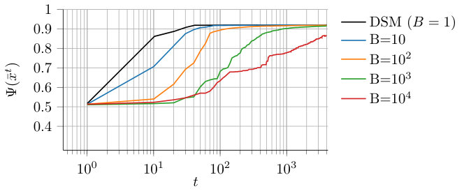 Figure 1
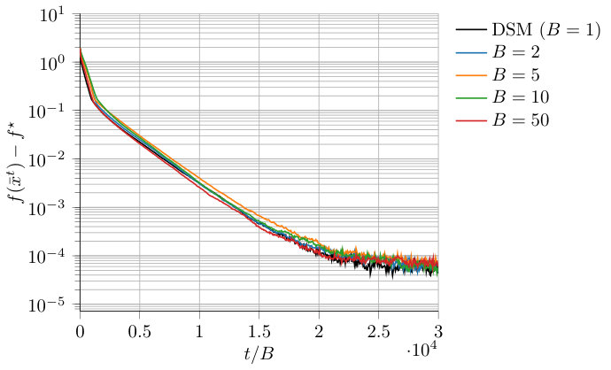 Figure 2
Peer Reviews
No public reviews on file for this paper yet. If you reviewed it on a platform where reviews are public (OpenReview, ICLR, NeurIPS, ICML), you can paste yours below so the community can read it here.
Videos
No videos yet. Explain this paper in a talk, walkthrough, or lecture? Add one.
Randomized Block Proximal Methods
for Distributed Stochastic Big-Data Optimization
Francesco Farina F. Farina is in the Artificial Intelligence and Machine Learning group at GSK. However, this work was carried out while the author was at the Department of Electrical, Electronic and Information Engineering “G. Marconi”, Università di Bologna, Bologna, Italy. email: [email protected]
Giuseppe Notarstefano G. Notarstefano is with the Department of Electrical, Electronic and Information Engineering “G. Marconi”, Università di Bologna, Bologna, Italy. email: [email protected]
Abstract
00footnotetext: A preliminary version of this work has appeared in the Proceedings of the 58-th Control and Decision Conference (CDC 2019) [1]. The current article consider a more general problem set-up, namely a constrained stochastic optimization one. Also the proposed algorithm is more general since local updates are based on generic proximal mappings, agents can be awake or idle at each iteration, blocks can be drawn according to locally defined (possibly non uniform) probability distributions and local stepsize sequences can be employied. Furthermore, the convergence analysis is also carried out under the assumption of constant stepsizes and an explicit convergence rate is provided. Finally, all the complete theoretical proofs are reported.00footnotetext: This result is part of a project that has received funding from the European Research Council (ERC) under the European Union’s Horizon 2020 research and innovation programme (grant agreement No 638992 - OPT4SMART).00footnotetext: ©2020 IEEE. Personal use of this material is permitted. Permission from IEEE must be obtained for all other uses, in any current or future media, including reprinting/republishing this material for advertising or promotional purposes, creating new collective works, for resale or redistribution to servers or lists, or reuse of any copyrighted component of this work in other works.00footnotetext: Digital Object Identifier 10.1109/TAC.2020.3027647
In this paper we introduce a class of novel distributed algorithms for solving stochastic big-data convex optimization problems over directed graphs. In the addressed set-up, the dimension of the decision variable can be extremely high and the objective function can be nonsmooth. The general algorithm consists of two main steps: a consensus step and an update on a single block of the optimization variable, which is then broadcast to neighbors. Three special instances of the proposed method, involving particular problem structures, are then presented. In the general case, the convergence of a dynamic consensus algorithm over random row stochastic matrices is shown. Then, the convergence of the proposed algorithm to the optimal cost is proven in expected value. Exact convergence is achieved when using diminishing (local) stepsizes, while approximate convergence is attained when constant stepsizes are employed. The convergence rate is shown to be sublinear and an explicit rate is provided in the case of constant stepsizes. Finally, the algorithm is tested on a distributed classification problem, first on synthetic data and, then, on a real, high-dimensional, text dataset.
1 Introduction
Recent years have witnessed a steadily growing interest in distributed learning and control over networks consisting of multiple smart agents. Several problems arising in this scenario can be formulated as distributed optimization problems which need to be solved by networks of agents. In this paper, we focus on the following stochastic big-data convex optimization problem, which is to be solved over a network of interconnected agents,
[TABLE]
where is a convex set, is a random variable and the functions are continuous, convex and possibly non smooth. The optimization variable is extremely high dimensional and with block structure, i.e., with being the dimension of the -th block and the number of blocks. Regarding the role of stochastic functions in the considered set-up, it is worth stressing that they allow agents to deal with various type of problems. Among the others, the case of learning problems involving massive datasets is of particular interest. In this case, the local objective function typically has the form , where , , are samples uniformly drawn from a certain dataset consisting of elements. When is very large it could be computationally infeasible to compute a subgradient of the entire . On the other side, given , computing a subgradient of is much simpler. Problems of this type are often referred to as sample average approximation problems [2]. Other relevant classes of problems include those of dynamic, or online, optimization problems in which samples generating functions are processed as they become available [3, 4] and settings in which only noisy subgradients of the objective functions are available [5].
Applying classical distributed algorithms to big-data problems may be infeasible due, e.g., to limitations in the communication bandwidth. In fact, they would require agents to communicate a prohibitive amount of data due to the high dimension of the decision variable. This calls for tailored distributed algorithms for big-data optimization problems in which only few blocks of the entire (local) solution estimate are sent to neighbors. Thus, the literature relevant to this paper can be divided in three main (partially overlapping) categories: stochastic optimization methods, block coordinate algorithms and primal distributed algorithms.
Stochastic optimization algorithms: To the best of our knowledge, the first work dealing with stochastic problems has been [6]. Since this seminal work, there has been a steady increase in the interest for this type of problems, and algorithms for solving them (see, e.g., [7] and references therein). Among the others, stochastic approximation approaches were presented in [8, 9] and stochastic mirror descent algorithms have been studied in [10, 11]. Stochastic gradient descent algorithms are particularly appealing in learning problems (see, e.g., [12]) in which extremely large datasets are involved, since they allow for batch processing of the data.
Block coordinate algorithms: Centralized block coordinate methods have a long history (see, e.g., [13] for a survey). They were firstly designed for solving smooth problems, but, in the last years, an increasing number of results have been provided to deal with nonsmooth objective functions. Two main rules for selecting the block to be updated have been studied: cyclic (or almost cyclic; see, e.g., [14]) or random. In the last case, randomized block coordinate algorithms have been proposed [15, 16, 17, 18, 19]. Particularly relevant for this paper is the work in [11], in which a stochastic block mirror descent method with random block updates is proposed. Parallel block coordinate methods are also a well established strand of optimization literature, see, e.g., [20]. The work in [21] applies to smooth convex functions, while the ones in [22, 23, 24] face up composite optimization problems. A unified framework for nonsmooth optimization using block algorithms has been studied in [25] for centralized and parallel set-ups.
Distributed algorithms: Many distributed optimization algorithms have been proposed in recent years. In [26] a distributed gradient descent algorithm was firstly introduced, which is capable to deal with both deterministic and stochastic convex optimization problems. When the problems to be solved involve nonsmooth objective functions, subgradient-based algorithms have been designed. First examples of such algorithms appeared in [27, 28, 29], while recent advances involve more sophisticated protocols, to deal with directed communication [30, 31, 32, 33, 34]. Many distributed algorithms involving proximal operations have also been proposed (see, e.g.,[35] for a survey on proximal algorithms). Among the others, a proximal gradient method was developed in [36] to deal with unconstrained problems, while in [37, 38] proximal algorithms have been presented to deal with constrained optimization. The stochastic setting has also been treated [5, 39, 40, 41, 42, 43, 44]. In particular, a stochastic subgradient projection algorithm appeared in [5], while a stochastic distributed mirror descent was proposed in [44]. Distributed algorithms over random networks are also relevant to this paper. In [45], consensus protocols were studied using random row-stochastic matrices, while in [46] a distributed subgradient method over random networks with underlying doubly stochastic matrices has been proposed. Distributed algorithms dealing with block communication have started to appear only recently. A block gradient tracking scheme has been presented in [47] for nonconvex problems with nonsmooth regularizers, while [48] proposes an asynchronous algorithm for nonconvex optimization based on the method of multipliers, which is implementable block-wise. A randomized block-coordinate algorithm for smooth problems with common cost function and linear constraints has been presented in [49].
In this paper, we introduce the Distributed Block Proximal Method, which models a class of distributed proximal algorithms, with block communication, for solving stochastic big-data convex optimization problems with nonsmooth objective function. The communication network is modeled as a directed graph admitting a doubly stochastic weight matrix. At each iteration, each node is awake with a certain probability (and idle otherwise). If awake, it performs a consensus step, computes a stochastic subgradient of a local objective function, and performs a proximal-based update (depending on the computed subgradient and on a local stepsize) on a randomly chosen block only. Then, it exchanges with its neighbors only the updated block of the decision variable, thus requiring a small amount of communication bandwidth. We also present three special instances of the proposed algorithm. In the first one, the proximal mapping is based on the squared 2-norm, thus leading to explicit block subgradient steps. In the other two, smooth objective functions and separable (possibly nonsmooth) ones are considered. In both these cases the computational load at each node in the network can be further reduced with respect to the general algorithm. We point out that no global parameter is required in the evolution of the algorithms. In fact, each node is awake and selects blocks with locally defined probabilities, and uses local stepsizes. The block-wise updates and the communication of a single block induce nontrivial technical challenges in the algorithm analysis. On this regard, it is worth noting that, despite the double stochasticity of the weight matrix, the consensus step on each block turns out to be performed using a sequence of random row-stochastic matrices. The analysis for the Distributed Block Proximal Method is carried out in two parts. First, the convergence properties of a dynamic block consensus protocol over random graphs are studied, by building on block-wise, perturbed consensus dynamics with random matrices. A bound on the expected distance from consensus is provided, which is then specialized to the cases of constant and diminishing stepsizes respectively. Then, a bound on the expected distance from the (globally) optimal cost is provided by properly bounding errors due to the block-wise update and exploiting the probability of drawing blocks. When constant stepsizes are used, approximate convergence (with a constant error term) to the optimal cost is proven in expected value, while asymptotic exact convergence is reached for diminishing stepsizes. Finally, we provide an explicit convergence rate for the proposed algorithm when using constant stepsizes. The rate is sublinear, even though a linear term is present, which can be predominant in the first iterations.
The paper is organized as follows. The problem set-up is introduced in Section 2 along with some preliminary results. In Section 3, the Distributed Block Proximal Method is presented and three special algorithm instances are given in Section 4. Then, the algorithm is analyzed in Section 5. Finally, a numerical example involving a distributed classification problem over a syntetic and a real, high-dimensional, text document datasets is dispensed in Section 6 and some conclusions are drawn in Section 7.
2 Set-up and preliminaries
2.1 Notation and definitions
Given a vector , we denote by the -th block of , i.e., given a partition of the identity matrix , with for all and , it holds and . Moreover we denote by the 2-norm of . Given a vector , with scalar blocks, we define
[TABLE]
Given a vector , we denote by the -th block of . Moreover, given a constant , and an index , we denote by , to the power of , while given a sequence , we denote by the -th element of the sequence. Given a matrix , we denote by (or ) the element of located at row and column . Given two matrices and , we write if for all and . Given two vectors we denote by their scalar product. Given a discrete random variable , we denote by the probability of to be equal to . Given a nonsmooth function , we denote by its subdifferential computed at , and by the subdifferential of with respect to the -th block of .
We say that a directed graph contains a spanning tree if for some there exists a directed path from the vertex to all other vertices . Given a nonnegative matrix and some , we denote by the matrix whose entries are defined as
[TABLE]
We say that contains a -spanning tree if the graph induced by contains a spanning tree.
2.2 Distributed stochastic optimization set-up
As anticipated in the introduction, we consider the following optimization problem,
[TABLE]
We recall that is a random variable, functions are continuous, convex and possibly nonsmooth for every , and . We let and . Moreover, is a solution of problem (1). The optimization variable has a block structure, i.e.,
[TABLE]
with for all and . We make the following assumption on the problem structure
Assumption 1** (Problem structure).**
- (A)
The constraint set has the block structure
[TABLE]
where, for , the set is closed and convex, and . 2. (B)
Let (resp. ) be a subgradient of (resp. ) computed at . Then, is an unbiased estimator of the subgradient of , i.e.,
[TABLE] 3. (C)
There exist constants and such that
[TABLE]
for all and , for all .
Notice that, if , Assumption 1(A) is clearly satisfied. Moreover, let us denote by the -th block of and let be a subgradient of computed at . Then, Assumption 1(C) implies that for all and . Moreover, let and . Then, and for all .
Problem (1) is to be solved in a distributed way by a network of agents. Each agent in the network is assumed to know only a portion of the entire problem, namely agent knows and the constraint set only. We make the following assumption on the network structure.
Assumption 2** (Communication structure).**
- (A)
The network is modeled through a weighted strongly connected directed graph with , and being the weighted adjacency matrix. We denote by the set of out-neighbors of node , i.e., . Similarly, the set of in-neighbors of node is defined as . 2. (B)
For all , the weights of the weight matrix satisfy
- (i)
if , if and only if ; 2. (ii)
there exists a constant such that and if , then ; 3. (iii)
and .
A function is associated to the -th block of the optimization variable for all . Let the function , be continuously differentiable and -strongly convex. Functions are sometimes referred to as distance generating functions. Then, we define the proximal function, also called Bregman’s divergence, associated to as
[TABLE]
for all . The following assumption is made on the functions .
Assumption 3** (Bregman’s divergence separate convexity).**
For all , the function satisfies
[TABLE]
where and for all .
Notice that the above assumption is satisfied by many functions (such as the quadratic function, the Boltzmann-Shannon entropy and the exponential function) and conditions on the functions guaranteeing (2) can be provided (see [50]). Finally, given , and , the proximal mapping associated to is defined as
[TABLE]
2.3 Preliminary results
Consider a stochastic, discrete-time dynamical system evolving according to
[TABLE]
where is a sequence of random row-stochastic matrices. Let be a probability space. We assume that the sequence forms an adapted process, i.e., is a stochastic process defined on , is a filtration (i.e., and for all ) and is measurable with respect to . Given a sequence of matrices , let us define the transition matrix from iteration to iteration as
[TABLE]
Then, the following result, adapted from [45, Theorem 3.1], holds true for system (4).
Lemma 1** ([45, Theorem 3.1]).**
Consider system (4). If there exist , such that contains a -spanning tree for each , and for each , then, for any given initial distribution of with (which is independent of ), and any , it holds
[TABLE]
where and .
Finally, the following three results will be useful in the rest of the paper.
Lemma 2**.**
Given a scalar , it holds that
- (i)
for any , 2. (ii)
*for any , *
Lemma 3** ([5, Lemma 3.1]).**
Let be a scalar sequence.
- (i)
If and then . 2. (ii)
*If , and , then . *
Lemma 4** (Tower property of conditional expectation).**
Let be a random variable defined on a probability space . Let . Then,
3 Distributed Block Proximal Method
The Distributed Block Proximal Method for solving problem (1) in a distributed way is now introduced. The algorithm works as follows. Each agent maintains a local solution estimate and a local copy of the estimates of its in-neighbors. Let us denote by the copy of the solution estimate of agent at agent . At the beginning, each node initializes its state with a random (bounded) initial condition which is then shared with its neighbors. At each iteration each agent is awake with probability and idle with probability . Thus, the proposed algorithm models a particular type of asynchrony in which the communication graph is fixed and agents can communicate or not with their neighbors with a certain probability. If agent is awake, it picks randomly a block , some , and performs two updates:
- (i)
it computes a weighted average of its in-neighbors’ estimates , ; 2. (ii)
it computes by updating the -th block of through a proximal mapping step and leaving the other blocks unchanged.
Then, it broadcasts to its out-neighbors. We model the status (awake or idle) of each node at each iteration through a random variable which is (corresponding to being awake) with probability and [math] with probability . A pseudocode of the method is reported in Algorithm 1.
Notice that all the quantities involved in the above algorithm are local for each node. In fact, each node has locally defined probabilities (both of awakening and block drawing) and local stepsizes.
Moreover, it is worth noting that, despite node receives from each only the block , the consensus step (6) is in fact performed by using the entire . Indeed, the other blocks have not changed since the last time they have been received. This is formalized in the next result.
Lemma 5**.**
Let Assumption 2 hold. Then for all . Moreover, Algorithm 1 can be compactly rewritten as follows. For all and all , if ,
[TABLE]
else, .
Proof.
The fact that for all and all follows immediately from the evolution of the algorithm. In fact, the received block is the only block that node has modified in the last iteration, while the others have remained unchanged. Hence, since the graph is fixed, it is clear that for all and all . The reformulation of Algorithm 1 as (8)-(9) is then immediate from Assumption 2(B). ∎
In virtue of the previous result, in order to lighten the notation in the subsequent analysis, we will use (8)-(9) in place of Algorithm 1, by making the block communication implicit.
As for the block-wise proximal update (9), the -th block of a whole stochastic subgradient computed at is used. Unfortunately, computing a subgradient with respect to the -th component only is, in general, not equivalent to picking the -th block of a whole subgradient . In fact, in general it holds that, picking ,…, does not imply . This will turn out to be extremely important in the subsequent analysis. If functions are separable on the blocks, then, only the subgradient with respect to the -th component can be computed. Similarly, if the functions are smooth, the -th block of the gradient can be directly computed as the gradient with respect to that block. In these cases, the computational load at each node can be further reduced, as it will be shown in Section 4.
The last key feature of the Distributed Block Proximal Method involves the consensus step (8). Let be the vector stacking the -th component of all the , i.e., . Also, let be a diagonal matrix in which the -th element of the diagonal is set to if and , and it is set to [math] otherwise, i.e.,
[TABLE]
Finally, let . Now, consider a consensus protocol associated to the Distributed Block Proximal Method, i.e.,
[TABLE]
This system can be rewritten in terms of as
[TABLE]
where . It can be easily verified that, for all and , the matrix is row-stochastic but not doubly stochastic anymore (unless all nodes select the same block at some iteration ).
Remark 1*.*
It is worth noting that the proposed algorithm, besides being easy to implement, considers challenges that cannot be addressed by other block-wise distributed algorithms [47, 48, 49]. In particular, none of those works deals with stochastic problems. Moreover, in [47] composite objective functions with non-smooth components are considered but the non-smooth part must be common to all the agents. In [48, 49] at least differentiability of the objective is required. Finally, in our algorithm, all the algorithm parameters are local.
4 Special instances
In this section, three special cases of the Distributed Block Proximal Method are presented. The first one is obtained by choosing the squared 2-norm as distance generating function, while the other two result from smooth and separable objective functions respectively.
4.1 Distributed Block Subgradient Method
By using for all , and assuming , the proximal mapping (3) has an explicit analytical solution and the update step (7) becomes
[TABLE]
Notice that, the proximal step becomes a subgradient step on a single block of the optimization variable. Thus, we call Distributed Block Subgradient Method the resulting algorithm, i.e., the one obtained by replacing (7) with (10) in Algorithm 1. Notice that, in this case, it holds that, for all , the strong convexity parameter is , thus resulting in special bounds in the subsequent algorithm analysis.
4.2 Smooth functions
The update of the solution estimate in (7) requires, in general, for node at iteration , the computation of an entire stochastic subgradient at the point . However, only the -th block of the computed subgradient is used in the update step. When a function is smooth, however, the -th block of its gradient can be directly computed as the gradient of with respect to the -th block of the optimization variable and (7) can be replaced by
[TABLE]
where denotes the (partial) gradient of with respect to the -th block of the optimization variable. Thus, when smooth functions are involved in the problem, the computational load can be reduced by avoiding the computation of the entire (sub)gradient.
4.3 Separable functions
When functions are separable, i.e.,
[TABLE]
the Distributed Block Proximal Method can be further simplified, allowing for an extra reduction of the computational load at each iteration at a given node. In fact, it holds that , and hence where is a subgradient of . This implies that and, thus, only the -th block of is needed in order to compute and hence . Thus the Distributed Block Proximal Method can be simplified by allowing nodes with a separable function to reduce their computational load. In particular, assume the cost function of node to be separable. Then, a single block of can be updated at each iteration and a subgradient can be directly computed for the corresponding block, without computing an entire subgradient. Hence, the algorithm can be rewritten, by using the equivalent formulation in Lemma 5, as follows. If ,
[TABLE]
else, .
5 Algorithm analysis
In this section, the convergence of the Distributed Block Proximal Method is proven in expected value. The proof consists of two main parts. In the first one the consensus of the agents’ solution estimates is shown, while in the second one convergence towards the optimal cost is proven. Both results are given, at first, in a general form and, then, specialized to the case of constant stepsizes (in which convergence to a neighborhood is proven) and diminishing stepsizes (in which exact asymptotic convergence is reached).
Define , and . We summarize in the following two assumptions, the two different choices for the stepsize sequences we consider in the following analysis.
Assumption 4** (Constant stepsize).**
The sequences satisfy for all and all .
Assumption 5** (Diminishing stepsize).**
The sequences satisfy
[TABLE]
for all . Moreover, for all and all .
Notice that, under Assumption 4, and for all , while, under Assumption 5 it can be easily verified that
[TABLE]
and
[TABLE]
Define the vector stacking all local solution estimates as , and the average (over the agents) of the local estimates at as
[TABLE]
Then, we make the following assumption on the random variables involved in the algorithm.
Assumption 6** (Random variables).**
- (A)
For a given , the random variables and are independent and identically distributed for all . 2. (B)
For a given , the random variables , and are independent of each other for all . 3. (C)
There exist constants such that for all and hence .
Before proceeding with the algorithm analysis, let us provide a preliminary instrumental result. Define and . Then, the following result applies.
Lemma 6**.**
Let Assumptions 1(A) and 1(C) hold. Then,
[TABLE]
for all , where .
Proof.
The first order necessary optimality condition on (9) for reads
[TABLE]
for all . Notice now that, by definition, , since it is a weighted average of points lying in . Thus, by taking , one obtains
[TABLE]
where we have used the strong convexity of . By rearranging the terms, one has
[TABLE]
and hence,
[TABLE]
Now, by taking the expected value and using the subgradient boundedness from Assumption 1(C), one gets
[TABLE]
thus concluding the proof. ∎
5.1 Dynamic consensus with random matrices
In this section we show that the sequences and computed by each agent in the network asymptotically achieve consensus in expected value when using diminishing stepsizes. Moreover, an upper bound on the distance from consensus is provided in the case of constant stepsizes.
Let be the set of estimates generated by the Distributed Block Proximal Method up to iteration (which is indeed a filtration). Moreover, define the probability of node to both be awake and pick block at each iteration as
[TABLE]
Then, the following lemma provides a bound on the expected distance between and the average (defined in (14)).
Lemma 7**.**
Let Assumptions 1(C), 2, 6 hold. Then, there exist constants and such that
[TABLE]
for all and all .
Proof.
For the sake of presentation, assume that the blocks are scalars, i.e., . Let us recall that defines the vector stacking the -th component of all the , i.e., , while the matrix is a diagonal matrix in which the -th element of the diagonal is set to if and and it is set to [math] otherwise, i.e.,
[TABLE]
Consistently, we let . Notice that, for all , is a random matrix whose diagonal element is with probability and [math] with probability . Define
[TABLE]
Then, by using Assumption 6(A), it can be verified that
[TABLE]
and, similarly,
[TABLE]
for all .
Now, Algorithm 1 can be rewritten with respecte to as
[TABLE]
where is, by definition, a row-stochastic matrix, and . Now, by recursively applying (21), it holds that
[TABLE]
where is the transition matrix from iteration to iteration associated to the matrices , . Moreover, by applying the operator on both sides (recall that ), one has
[TABLE]
Notice now that, by using (19) and (20),
[TABLE]
for all . It can be seen that such a matrix is row stochastic and contains a -spanning tree with (since from Assumption 2 the matrix contains a spanning tree), where is defined in Assumption 2(B). Moreover, by Assumption 6(A), is a sequence of i.i.d. random matrices with . Hence, from Lemma 1, by taking the expectation on both sides of (22), we get
[TABLE]
where we used the fact that, from Lemma 6,
[TABLE]
Let us now define
[TABLE]
Since , for all , we have that
[TABLE]
for all . Notice now that, by definition and . Hence,
[TABLE]
Finally, since , one has
[TABLE]
where . The proof is concluded by using Assumption 6(C). ∎
Moreover, the expected value of the distance between and can be bounded, by exploiting the convexity of the norm and using Lemma 7, as stated in the next result.
Lemma 8**.**
Let Assumptions 1(C), 2, 6 hold. Then,
[TABLE]
for all and all .
Proof.
Form the definition of and using the convexity of the norm, one has
[TABLE]
By taking the expected value on both sides and using Lemma 7, the proof follows by noting that from Assumption 2(B). ∎
5.1.1 Constant stepsize
The following two results respectively provide an upper bound on the distance of from as and characterize the quantity for each in the case of constant stepsizes.
Lemma 9**.**
Let Assumptions 1(C), 2, 4, 6 hold. Then, there exist constants and such that
[TABLE]
for all , with
[TABLE]
Proof.
Equation (18) in Lemma 7 consists of three terms. For the first one, , since . For the second term , by Assumption 4 and Lemma 3, one has that . The proof is completed by noting that, under Assumption 4 the last term is constant. ∎
Lemma 10**.**
Let Assumptions 1(C), 2, 4, 6 hold. Then,
[TABLE]
for all , with
[TABLE]
Proof.
By using Assumption 6(C), for , one has
[TABLE]
Hence, and, from Lemma 7, we have
[TABLE]
where in the last line we have rearranged the summations. Now, by noting that
[TABLE]
and using Lemma 2 the result follows through straightforward manipulations. ∎
Notice that in virtue of Lemma 8, by using the same reasoning used in the previous two results it is possible to show that
[TABLE]
and
[TABLE]
These bounds will be used in the following optimality analysis.
5.1.2 Diminishing stepsize
When adopting diminishing stepsizes, asymptotic (exact) consensus can be reached as stated in the following result.
Lemma 11**.**
Let Assumptions 1(C), 2, 5, 6 hold. Then,
[TABLE]
for all .
Proof.
The proof is based on the same arguments as in Lemma 9. By noting that as and that, under Assumption 5, from Lemma 3, , the result follows. ∎
The next result shows that is a summable series for all . Notice that this result does not hold in the case of constant stepsizes.
Lemma 12**.**
Let Assumptions 1(C), 2, 5, 6 hold. Then,
[TABLE]
for all .
Proof.
As for , from (5.1.1) we have , while, for , from Lemma 7 it holds that
[TABLE]
Since, by Assumption 5, for all , one has
[TABLE]
and then,
[TABLE]
Now, from Assumption 6(C), . Moreover, by using Assumption 5 and Lemma 3, we have . Finally, by Assumption 5, , so that, from Lemma 3, , thus concluding the proof. ∎
As in the case of constant stepsizes, thanks to Lemma 8, it can be shown that and .
5.2 Optimality
In this section, we show the convergence of the Distributed Block Proximal Method. First, a bound on the expected distance from the optimal cost at iteration is given without any assumption on the stepsize sequence. Then, it is shown that such a distance goes to [math] as for diminishing stepsizes, while it is upper bounded by a finite quantity for constant stepsizes and an explicit convergence rate is provided.
We start by defining the Ljapunov function
[TABLE]
and . Moreover, given a sequence of points , we define
[TABLE]
Then, the following result holds true.
Theorem 1**.**
Let Assumptions 1, 2, 3, 6 hold. Then,
[TABLE]
Proof.
In order to simplify the notation, let us denote and . From the convexity of we have that, at a given iteration ,
[TABLE]
Now, we make some manipulation on the term :
[TABLE]
where we have used multiple times the convexity of (and of each ) and the subgradient boundedness (Assumption 1(C)). Let us now study the term in (31). By writing the optimality condition for the proximal mapping in the update (9), if , one has
[TABLE]
Hence,
[TABLE]
Thus, from (33) and by using (27), one has that, if , it holds
[TABLE]
while, if ,
[TABLE]
Now, by taking the expected value of conditioned to , one obtains
[TABLE]
and hence, by substituting (34) and (35) in (36),
[TABLE]
Notice now that
[TABLE]
Moreover, by noting that it holds that and and by substituting (38) in (37), we obtain
[TABLE]
where in the last inequality we used the separate convexity of from Assumptions 3 and the fact that (Assumption 1(C)), and (Assumption 1(B)). Now, by summing over ,
[TABLE]
where in the last inequality we used the convexity of . Taking the expected value conditioned to on both sides of (40), using and Lemma 4, gives
[TABLE]
and, rearranging the terms,
[TABLE]
Now, by summing over , and noting that ,
[TABLE]
Moreover, by taking the expected value over ,
[TABLE]
Notice now that, since by definition for all and , we have
[TABLE]
Finally, by combining (30), (31), (41) and (42) one obtains (29). ∎
A similar result can be given also in terms of the sequences of local solution estimates as formalized in the next result.
Corollary 1**.**
Let Assumptions 1, 2, 3, 6 hold. Then,
[TABLE]
for all .
Proof.
The proof follows the same line of the one of Theorem 1, by noting that
[TABLE]
so that in place of (30), one has
[TABLE]
for all . ∎
The previous two results hold true without making any assumption on the local stepsize sequences. In the next two subsections the general result of Theorem 1 is specialized to the case of constant and diminishing stepsizes respectively.
5.2.1 Constant stepsizes
In the case of constant (local) stepsizes, convergence with a constant error is attained with an explicit sublinear convergence rate.
Theorem 2**.**
Let Assumptions 1, 2, 3, 4, 6 hold. Then, there exist constants and such that
[TABLE]
for all , with
[TABLE]
Proof.
By exploiting Assumption 4, Lemma 10 and Lemma 8, from (43) one obtains
[TABLE]
which, by rearranging the terms, leads to
[TABLE]
thus concluding the proof. ∎
The previous result shows that, when constant stepsizes are employed, the value of converges to plus a constant error, which can be retrieved from (44) by taking the limit for , i.e., with the explicit expression for being
[TABLE]
It is worth noting that the bound decreases with the maximum stepsize . Regarding the convergence rate, it is sublinear . However, in the first iterations, the term can be dominant (if ), thus leading to a linear rate at the beginning of the algorithm (as it will be shown in the numerical example). Notice that (and hence the convergence rate) depends both on the number of blocks and on the local probabilities of being awake and drawing blocks. The local probabilities appear in and (implicitly) in the constant . In fact, is related to the randomness of the matrices , which depend on such probabilities. In particular notice that, if the rate is similar to those obtained in [27], in which the proximal mapping is used. Clearly, one may argue that the best rate is achieved by using a single block and hence, communicating in terms of blocks is useless. This is true only if we assume an infinite bandwidth to be available in the communication channels (i.e, transmitting the entire optimization variable or a single block of it requires the same amount of time). However, in typical real world scenarios this is not true and data that exceed the communication bandwidth are transmitted sequentially. If only one block fits the communication channel, our algorithm allows to perform an update at each communication round, while classical ones would need communication rounds per update. Moreover, in the proposed algorithm, typically, the local computation time at each iteration is not negligible, since a minimization problem is to be solved at every step (see (7)). Solving such an optimization problem on the entire optimization variable or on a single block of it clearly results in completely different computational times, which are clearly lower in the case of block-wise updates. Thus, the benefits of using block-wise updates and communications make the Distributed Block Proximal Method well suited for big-data optimization problems.
5.2.2 Diminishing stepsizes
In the case of diminishing (local) stepsizes, asymptotic convergence to the optimal cost can be reached.
Theorem 3**.**
Let Assumptions 1, 2, 3, 5, 6 hold. Then,
[TABLE]
for all
Proof.
The proof follows by taking the limit for , and using Assumption 5 and Lemma 12 in (43). ∎
Remark 2*.*
We point out that, similarly to, e.g., [37, 11], one can introduce a running averaging mechanism by defining and provide the convergence results in terms of , in place of . The convergence proof would follow almost the same line with some adjustments in (30)-(31) (see [11]). However, running averaging mechanisms typically lead to a significantly slower convergence rate. In light of this, we provided our results in terms of .
6 Numerical example
Consider a soft margin classification problem in which each agent has training samples each of which has an associated binary label for all . The goal of the network is to build a linear classifier from the training samples, i.e., to find a hyperplane of the form , with and , which better separates the training data. Let us define and . Then, the solution to this problem can be determined by solving the following SVM problem
[TABLE]
where is the regularization weight. Problem (45) can be written in the form of problem (1) by defining and
[TABLE]
for all . Notice that, as long as each data is uniformly drawn from the dataset, Assumption 1(B) is satisfied.
In the next two sections we will test the Distributed Block Subgradient Method in the presented scenario, first on a synthetic dataset and then on real-world dataset composed of text documents. In both cases we consider a system with processors. The proposed distributed algorithm has been implemented by using the Python package DISROPT [51], and each processor has been assigned an agent.
6.1 Synthetic dataset
In order to show how the algorithm performs for different number of blocks, let us consider a relatively low-dimensional problem with and evaluate the algorithm performance for different number of blocks, namely . We generate a synthetic dataset (with ) composed of 240 points (taken from two clusters corresponding to labels and respectively) and assign of them to each agent, i.e., . Finally, we set , a common (constant) stepsize , for all and all and for all and all . Regarding the communication graph, it has is generated according to an Erdős-Rènyi random model with connectivity parameter . The corresponding weight matrix is built by using the Metropolis-Hastings rule. The evolution of the cost error adjusted with respect to the number of blocks is reported in Figure 1 for the considered block numbers. The results confirm the discussion carried out in Section 5.2.1 about the role of block communications. In fact, when normalizing the number of iterations with respect to the number of blocks, the convergence rates for the considered number of blocks are comparable. Moreover, the convergence rate exhibits the properties shown in Section 5.2.1. In fact, it is linear at the beginning and becomes sublinear after some iterations. Moreover, as expected when using constant stepsizes, convergence is reached with a constant error.
6.2 Text classification
Let us now consider a real-world scenario in which the local training samples are drawn from a dataset of texts. In particular, we pick the 20 newsgroups dataset, a dataset consisting of 18,846 newsgroup posts belonging to topics. Texts are represented by tf-idf on a dictionary of 130,107 words, so that each sample is a vector in . Agents have to learn to classify posts belonging to the class sci.med from the others. Thus, in order to perform a binary classification, we assign the label to samples belonging to the class sci.med, and to all the other samples. In this scenario, the considered agents, are connected over a balanced directed graph, generated according to a binomial random model with connectivity parameter and each agent is awake with probability . The entire dataset is split to assign almost the same number of samples to each agent. We run the algorithm for iterations and for different number of blocks, namely . Moreover, we set in problem (45), and we select a common (constant) stepsize and for all and all . Differently from the previous example over synthetic data, in this case computing the exact (centralized) solution of the considered problem is computationally intractable, due to the high dimension of the decision variable (130,107) and the large number of samples (18,146). Thus, the performance of the algorithm are evaluated in terms of the accuracy of the average of the produced solution estimates , i.e., the number of samples of the dataset that are correctly classified through the hyperplane defined by . The results are reported in Figure 2.
7 Conclusions
In this paper, we introduced a class of distributed block proximal algorithms for solving stochastic big-data convex optimization problems over networks. In the addressed optimization set-up the dimension of the decision variable is very high and the (stochastic) cost function may be nonsmooth. The main strength of the proposed algorithms is that agents in the network can communicate a single block of the optimization variable per iteration. Under the assumption of diminishing stepsizes, we showed that the agents in the network asymptotically agree on a common solution which is cost-optimal in expected value. When employing constant stepsizes approximate convergence is attained with a constant error on the optimal cost and an explicit convergence rate is provided. Special instances of the algorithm are presented for particular classes of problems. Finally, the proposed algorithm, has been numerically evaluated on a distributed classification problem over both a synthetic dataset and a real, high-dimensional, text document dataset.
The reference list from the paper itself. Each links out to its DOI / PubMed record.
- 1[1] F. Farina and G. Notarstefano, “A randomized block subgradient approach to distributed big data optimization,” in 2019 IEEE 58th Conference on Decision and Control (CDC) , 2019.
- 2[2] A. J. Kleywegt, A. Shapiro, and T. Homem-de Mello, “The sample average approximation method for stochastic discrete optimization,” SIAM Journal on Optimization , vol. 12, no. 2, pp. 479–502, 2002.
- 3[3] L. Xiao, “Dual averaging methods for regularized stochastic learning and online optimization,” Journal of Machine Learning Research , vol. 11, no. Oct, pp. 2543–2596, 2010.
- 4[4] K. I. Tsianos and M. G. Rabbat, “Consensus-based distributed online prediction and optimization,” in 2013 IEEE Global Conference on Signal and Information Processing , 2013, pp. 807–810.
- 5[5] S. S. Ram, A. Nedić, and V. V. Veeravalli, “Distributed stochastic subgradient projection algorithms for convex optimization,” Journal of optimization theory and applications , vol. 147, no. 3, pp. 516–545, 2010.
- 6[6] H. Robbins and S. Monro, “A stochastic approximation method,” The annals of mathematical statistics , pp. 400–407, 1951.
- 7[7] H. Kushner and G. G. Yin, Stochastic approximation and recursive algorithms and applications . Springer Science & Business Media, 2003, vol. 35.
- 8[8] A. Nemirovski, A. Juditsky, G. Lan, and A. Shapiro, “Robust stochastic approximation approach to stochastic programming,” SIAM Journal on optimization , vol. 19, no. 4, pp. 1574–1609, 2009.