TL;DR
This paper introduces an inexact block coordinate descent algorithm tailored for large-scale nonsmooth nonconvex optimization, emphasizing flexibility, fast convergence, and low complexity, with proven convergence guarantees.
Contribution
The paper presents a novel inexact block coordinate descent method that allows flexible approximation functions and guarantees convergence even without Lipschitz continuous gradients.
Findings
Algorithm demonstrates fast convergence in large-scale problems.
Applicable to signal processing and machine learning tasks.
Converges to stationary points even with inexact subproblem solutions.
Abstract
In this paper, we propose an inexact block coordinate descent algorithm for large-scale nonsmooth nonconvex optimization problems. At each iteration, a particular block variable is selected and updated by inexactly solving the original optimization problem with respect to that block variable. More precisely, a local approximation of the original optimization problem is solved. The proposed algorithm has several attractive features, namely, i) high flexibility, as the approximation function only needs to be strictly convex and it does not have to be a global upper bound of the original function; ii) fast convergence, as the approximation function can be designed to exploit the problem structure at hand and the stepsize is calculated by the line search; iii) low complexity, as the approximation subproblems are much easier to solve and the line search scheme is carried out over a properly…
Click any figure to enlarge with its caption.
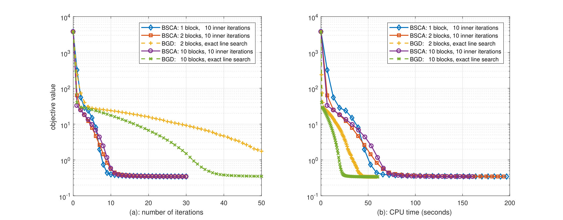 Figure 1
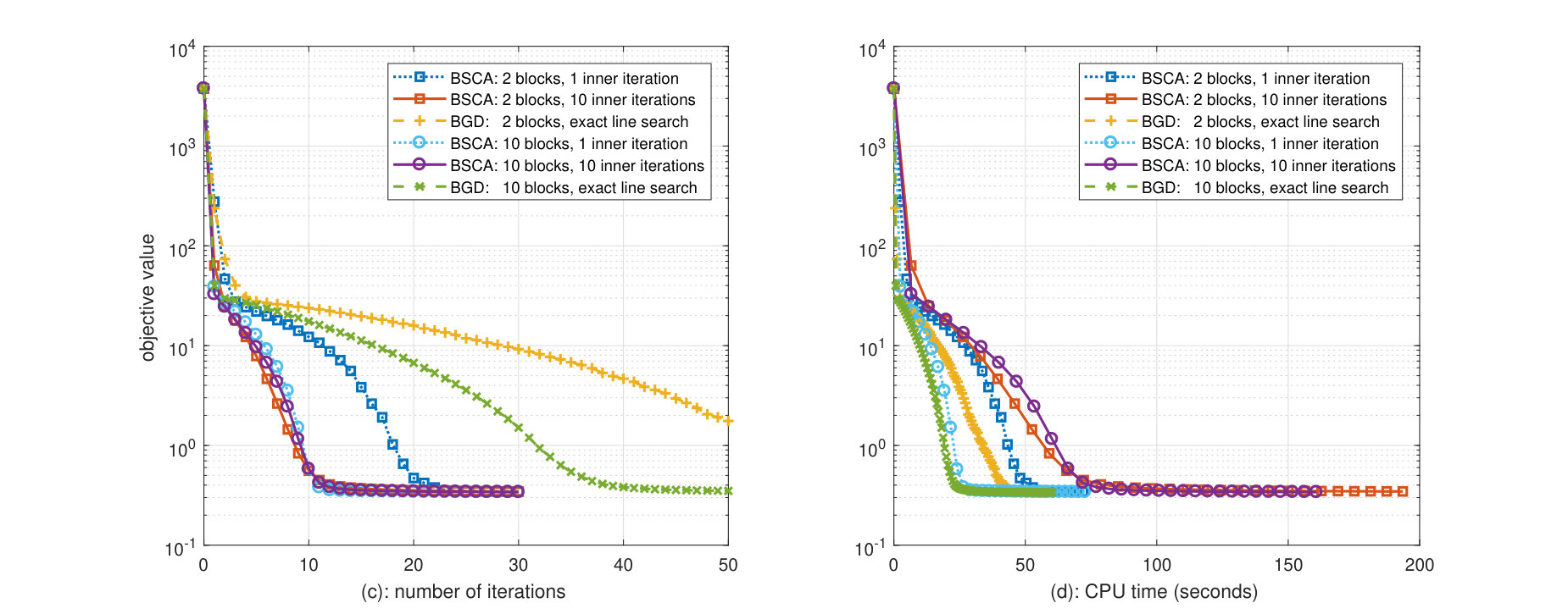 Figure 2
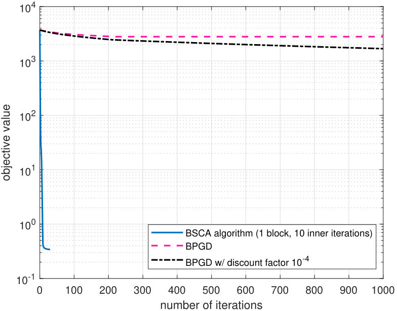 Figure 3
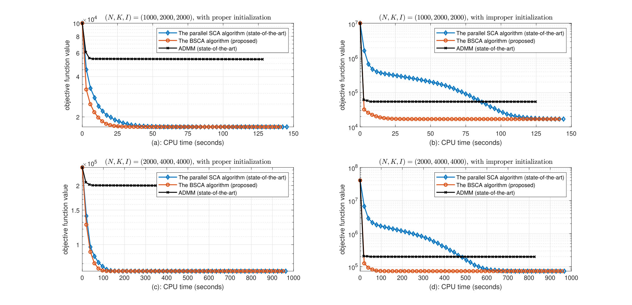 Figure 4
Peer Reviews
No public reviews on file for this paper yet. If you reviewed it on a platform where reviews are public (OpenReview, ICLR, NeurIPS, ICML), you can paste yours below so the community can read it here.
Code & Models
Videos
No videos yet. Explain this paper in a talk, walkthrough, or lecture? Add one.
Inexact Block Coordinate Descent Algorithms for Nonsmooth Nonconvex
Optimization
Yang Yang, Marius Pesavento, Zhi-Quan Luo, Bj rn Ottersten Y. Yang is with the Competence Center for High Performance Computing, Fraunhofer Institute for Industrial Mathematics, 67663 Kaiserslautern, Germany (email: [email protected]). His work is supported by the ERC project AGNOSTIC.M. Pesavento is with the Communication Systems Group, Technische Universit t Darmstadt, 64283 Darmstadt, Germany (email: [email protected]). His work is supported by supported by the EXPRESS project within the DFG priority program CoSIP (DFG-SPP 1798).Z.-Q. Luo is with Shenzhen Research Institute of Big Data, and the Chinese University of Hong Kong, Shenzhen, China (email: [email protected]). His work is supported by the leading talents of Guangdong province Program (No. 00201501), the National Natural Science Foundation of China (No. 61731018), the Development and Reform Commission of Shenzhen Municipality, and the Shenzhen Fundamental Research Fund (No. KQTD201503311441545).B. Ottersten is with University of Luxembourg, L-1855 Luxembourg (email: [email protected]). His work is supported by the ERC project AGNOSTIC.
Abstract
In this paper, we propose an inexact block coordinate descent algorithm for large-scale nonsmooth nonconvex optimization problems. At each iteration, a particular block variable is selected and updated by inexactly solving the original optimization problem with respect to that block variable. More precisely, a local approximation of the original optimization problem is solved. The proposed algorithm has several attractive features, namely, i) high flexibility, as the approximation function only needs to be strictly convex and it does not have to be a global upper bound of the original function; ii) fast convergence, as the approximation function can be designed to exploit the problem structure at hand and the stepsize is calculated by the line search; iii) low complexity, as the approximation subproblems are much easier to solve and the line search scheme is carried out over a properly constructed differentiable function; iv) guaranteed convergence of a subsequence to a stationary point, even when the objective function does not have a Lipschitz continuous gradient. Interestingly, when the approximation subproblem is solved by a descent algorithm, convergence of a subsequence to a stationary point is still guaranteed even if the approximation subproblem is solved inexactly by terminating the descent algorithm after a finite number of iterations. These features make the proposed algorithm suitable for large-scale problems where the dimension exceeds the memory and/or the processing capability of the existing hardware. These features are also illustrated by several applications in signal processing and machine learning, for instance, network anomaly detection and phase retrieval.
Index Terms:
Big Data, Block Coordinate Descent, Phase Retrieval, Line Search, Network Anomaly Detection, Successive Convex Approximation
I Introduction
In this paper, we consider the optimization problem
[TABLE]
where the function is proper, is smooth (but not necessarily convex), is proper, lower semicontinuous and convex (but not necessarily smooth), and the constraint set has a Cartesian product structure with being closed and convex for all . Such a formulation plays a fundamental role in signal processing and machine learning, and typically models the estimation error or empirical loss while is a regularization (penalty) function promoting in the solution a certain structure known a priori such as sparsity.
For a large-scale nonconvex optimization problem of the form (1), the block coordinate descent (BCD) algorithm has been recognized as an efficient and reliable numerical method. Its variable update is based on the so-called nonlinear best-response [1, 2, 3, 4, 5]: at each iteration of the BCD algorithm, one block variable, say , is updated by its best-response while the other block variables are fixed to their values of the preceding iteration
[TABLE]
That is, the best-response is the optimal point that minimizes with respect to (w.r.t.) the variable .
The BCD algorithm has several notable advantages. First of all, the subproblem (2) (w.r.t. a block variable ) is much easier to solve than the original problem (1) (w.r.t. the whole set of variables ), and the best-response even has a closed-form expression in many applications, for example LASSO [6]. It is thus suitable for implementation on hardware with limited memory and/or computational capability. Secondly, as all block variables are updated sequentially, when a block variable is updated, the newest value of other block variables is always incorporated. These two attractive features can sometimes lead to even faster convergence than their parallel counterpart, namely, the Jacobi algorithm (also known as the parallel best-response algorithm) [1].
In cases where the subproblems (2) are still difficult to solve and/or (sufficient) convergence conditions (mostly on the convexity of and the uniqueness of , see [7, 2, 8] and the references therein) are not satisfied, several extensions have been proposed. Their central idea is to solve the optimization problem (2) inexactly. For example, in the block successive upper bound minimization (BSUM) algorithm [3], a global upper bound function of is minimized at each iteration. Common examples are proximal approximations [8, 9] and, if is block Lipschitz continuous111The gradient is Lipschitz continuous if there exists a finite constant such that for all . It is block Lipschitz continuous if there exists a finite constant such that for all and and ., proximal-linear approximation [8, 10]. However, for the BSUM algorithm, a global upper bound function may not exist for some (and thus ).
The block Lipschitz continuity assumption is not needed if a stepsize is employed in the variable update. In practice, the stepsize can be determined by line search [11, 12]. Nevertheless, only a specific approximation of is considered, namely, quadratic approximation. Sometimes it may be desirable to use other approximations to better exploit the problem structure, for example, best-response approximation and partial linearization approximation when the nonconvex function has “partial” convexity (their precise descriptions are provided in Section III) . This is the central idea in recent (parallel) successive convex approximation (SCA) algorithms [13, 14, 15, 16, 17] and block successive convex approximation (BSCA) algorithms [3, 18, 19], which consist in solving a sequence of successively refined convex approximation subproblems. A new line search scheme to determine the stepsize is also proposed in [16, 17]: it is carried out over a properly constructed smooth function and its complexity is much lower than traditional schemes that directly operate on the original nonsmooth function [11, 13, 12]. For example, as we will see later in the applications studied in this paper, when represents a quadratic loss function, the exact line search has a simple analytical expression.
Nevertheless, existing BSCA schemes also have their limitations: the BSCA algorithm proposed in [3] is not applicable when the objective function is nonsmooth, and the convergence of the BSCA algorithms proposed in [18, 19] is only established under the assumption that is Lipschitz continuous and the stepsizes are decreasing. Although it is shown in [18] that constant stepsizes can also be used, the choice of the constant stepsizes depends on the Lipschitz constant of that is not easy to obtain/estimate when the problem dimension is extremely large.
The standard SCA and BSCA algorithms [12, 3, 18, 16, 17] are based on the assumption that the approximation subproblem is solved perfectly at each iteration. Unless the approximation subproblems have a closed-form solution, this assumption can hardly be satisfied by iterative algorithms that exhibit an asymptotic convergence only as they must be terminated after a finite number of iterations in practice. It is shown in [15, 19, 9] that convergence is still guaranteed if the approximation subproblems are solved approximately with a prescribed accuracy. However, the solution accuracy is specified by an error bound which is difficult to verify in practice. A different approach is adopted in [20, 21] where the optimization problem (2) is solved inexactly by running the (proximal) gradient projection algorithm for a finite number of iterations. Nevertheless, its convergence is only established for the specific application in nonnegative matrix factorization in [20] and the use of the (proximal) gradient projection can be restrictive.
In this paper, we propose a block successive convex approximation (BSCA) framework for the nonsmooth nonconvex problem (1) by extending the parallel update scheme in [16] to a block update scheme. The proposed BSCA algorithm consists in optimizing a sequence of successively refined approximation subproblems, and has several attractive features.
- i)
The approximation function is a strictly convex approximation of the original function and it does not need to be a global upper bound of the original function; 2. ii)
The stepsize is calculated by performing the (exact or successive) line search scheme along the coordinate of the block variable being updated and has low complexity as it is carried out over a properly constructed smooth function; 3. iii)
If the approximation subproblem does not admit a closed-form solution and is solved iteratively by a descent algorithm, for example the (parallel) SCA algorithm proposed in [16], the descent algorithm can be terminated after a finite number of iterations; 4. iv)
Convergence of a subsequence to a stationary point is established, even when is not multiconvex and/or is not block Lipschitz continuous.
These features are distinctive from existing works from the following aspects:
- •
Feature i) extends the BSUM algorithm [3] and BCD algorithm [8, (1.3b)] where the approximation function must be a global upper bound of the original function, [11, 12] and [18, 19] where the approximation functions must be quadratic and strongly convex, respectively;
- •
Feature ii) extends [18, 19] where decreasing stepsizes are used, and [11, 13, 12] where the line search is over the original nonsmooth function and has a high complexity;
- •
Feature iii) extends [19] where the approximation subproblems must be solved with increasing accuracy. We remark that this feature is inspired by [13], but we establish convergence under weaker assumptions;
- •
Feature iv) extends [8, (1.3a)] where is multi-strongly-convex, [18, 19, 9] where must be Lipschitz continuous, [8, (1.3c)] and [10] where must be block Lipschitz continuous, and [13, 12] where line search over the original nonsmooth function is used. Nevertheless, the convergence of a subsequence is weaker than the convergence of the whole sequence established in [8, 9, 10].
These attractive features are illustrated by several applications in signal processing and machine learning, namely, network anomaly detection and phase retrieval.
The rest of the paper is structured as follows. In Sec. II, we give a brief review of the SCA framework proposed in [16]. In Sec. III, the BSCA framework together with the convergence analysis is formally presented. An inexact BSCA framework is proposed in Sec. IV. The attractive features of the proposed (exact and inexact) BSCA framework are illustrated through several applications in Sec. V. Finally some concluding remarks are drawn in Sec. VI.
*Notation: *We use , and to denote a scalar, vector and matrix, respectively. We use and to denote the -th element and the -th column of , respectively; is the -th element of where , and denotes all elements of except : . We denote and as the element-wise operation, i.e., and , respectively. Notation denotes the Hadamard product between and . The operator returns the element-wise projection of onto : . We denote as the vector that consists of the diagonal elements of and is a diagonal matrix whose diagonal vector is . We use to denote a vector with all elements equal to 1. The operator specifies the -norm of and it denotes the spectral norm when is not specified. denotes the soft-thresholding operator: .
II Review of the Successive Convex Approximation
framework
In this section, we present a brief review of (a special case of) the SCA framework developed in [16] for problem (1). It consists of solving a sequence of successively refined approximation subproblems: given at iteration , the approximation function of w.r.t. is denoted as , and the approximation subproblem consists of minimizing the approximation function over the constraint set :
[TABLE]
where satisfies several technical assumptions, most notably,
- •
Convexity222Please refer to [16, Sec. II] for optimization terminologies such as (strict, strong) convexity, descent direction and stationary point.: The function is convex in for any given ;
- •
Gradient Consistency: The gradient of and the gradient of are identical at , i.e., .
We have also implicitly assumed that exists. The approximation subproblem (3) can readily be decomposed into independent subproblems that can be solved in parallel: and
[TABLE]
Remark 1*.*
The approximation function in (3) is a special case of the general SCA framework developed in [16] because it is separable among the different block variables. More generally, , the approximation function of , only needs to be convex and differentiable with the same gradient as at , and it does not necessarily admit a separable structure.
Since is an optimal point of problem (3), we have
[TABLE]
where , and is due to the optimality of , the convexity of in and the gradient consistency assumption, respectively. Therefore is a descent direction of the original objective function in (1) along which the function value can be further decreased compared with [16, Prop. 1]. This motivates us to refine and define as follows:
[TABLE]
where is the stepsize that needs to be selected properly to yield a fast convergence.
It is natural to select a stepsize such that the function is minimized w.r.t. :
[TABLE]
and this is the so-called exact line search (also known as the minimization rule). For nonsmooth optimization problems, the traditional exact line search usually suffers from a high complexity as the optimization problem (6) is nondifferentiable. It is shown in [16, Sec. III-A] that the stepsize obtained by performing the exact line search over the following differentiable function also yields a decrease in :
[TABLE]
To see this, we remark that firstly, the objective function in (7) is an upper bound of the objective function in (6) which is tight at since is convex:
[TABLE]
Secondly, the objective function in (7) has a negative slope at as its gradient is equal to in (4). Therefore, and .
If the scalar differentiable optimization problem in (7) is still difficult to solve, the low-complexity successive line search (also known as the Armijo rule) can be used instead [16, Sec. III-A]: given scalars and , the stepsize is set to be , where is the smallest nonnegative integer satisfying
[TABLE]
where is the descent defined in (4).
The above steps are summarized in Alg. 1. As a descent algorithm, it generates a monotonically decreasing sequence , and every limit point of is a stationary point of (1) (see [16, Thm. 2] for the proof).
III The Proposed Block Successive Convex Approximation
Algorithms
From a theoretical perspective, Alg. 1 is fully parallelizable. In practice, however, it may not be fully parallelized when the problem dimension exceeds the hardware’s memory and/or processing capability. We could naively solve the independent subproblems in Step S1 of Alg. 1 sequentially, for example, in a cyclic order. Once all independent subproblems are solved, a joint line search is performed as in Step S2 of Alg. 1.** **However, when the approximation subproblem w.r.t. is being solved, the solutions of previous approximation subproblems w.r.t. are already available, but they are not exploited.
An alternative is to apply the BCD algorithm, where the variable is first divided into blocks and the block variables are updated sequentially. Suppose is being updated at iteration , the following optimization problem w.r.t. the block variable (rather than the full variable ) is solved while the other block variables are fixed:
[TABLE]
Convergence to a stationary point of problem (1) is guaranteed if, for example, is unique [2]. However, the optimization problem in (9) may still not be easy to solve. One approach is to apply Alg. 1 to solve (9) iteratively, but the resulting algorithm will be of two layers: Alg. 1 keeps iterating in the inner layer until a given accuracy is reached and the block variable to be updated next is selected in the outer layer.
To reduce the stringent requirement on the processing capability of the hardware imposed by the parallel SCA algorithms and the complexity of the BCD algorithm, we design in this section a BSCA algorithm: when the block variable is selected at iteration , all elements of are updated in parallel by solving an approximation subproblem w.r.t. (rather than the whole variable as in Alg. 1) that is presumably much easier to optimize than the original problem (9):
[TABLE]
Note that and defined in (10) is an approximation function of and at a given point , respectively. We assume that the approximation function satisfies the following technical conditions:
(A1) The function is strictly convex in for any given ;
(A2) The function is continuously differentiable in for any given and continuous in for any ;
(A3) The gradient of and the gradient of w.r.t. are identical at for any , i.e., ;
(A4) A solution exists for any .
Since the objective function in (10) is strictly convex, is unique. If , then is the optimal point of the optimization problem in (9) given fixed [16, Prop. 1]. We thus consider the case that , and this implies that
[TABLE]
It follows from the strict convexity of and Assumption (A3) that
[TABLE]
Combining (11) and (12), we readily see that is a descent direction of at along the coordinate of in the sense that:
[TABLE]
Then is updated according to the following expression: and
[TABLE]
In other words, only the block variable is updated while other block variables are equal to their value at the previous iteration. The stepsize in (14) can be determined along the coordinate of efficiently by the line search introduced in the previous section, namely, either the exact line search
[TABLE]
or the successive line search if the nonconvex differentiable function in (15) is still difficult to optimize: given predefined constants and , the stepsize is set to , where is the smallest nonnegative integer satisfying the inequality:
[TABLE]
where is the descent in (13). Note that the line search in (15)-(16) is performed along the coordinate of only.
At the next iteration , a new block variable is selected and updated. We consider two commonly used rules to select the block variable, namely, the cyclic update rule and the random update rule. Note that both of them are well-known (see [18, 19]), but we give their definitions for the sake of reference in later developments.
Cyclic update rule: The block variables are updated in a cyclic order. That is, we select the block variable with index
[TABLE]
Random update rule: The block variables are selected randomly according to
[TABLE]
and . Any block variable can be selected with a nonzero probability, and some examples are given in [19].
The proposed BSCA algorithm is summarized in Alg. 2, and its convergence properties are given in the following theorem.
Theorem 2**.**
Every limit point of the sequence generated by the BSCA algorithm in Alg. 2 is a stationary point of (1) (with probability 1 for the random update).
Proof:
See Appendix A. ∎
The existence of a limit point is guaranteed if the constraint set in (1) is bounded or the objective function has a bounded lower level set. A sufficient condition for the latter is that is coercive, i.e., as .
If is a global upper bound of , we can simply use a constant unit stepsize , that is,
[TABLE]
for the reason that the constant unit stepsize always yields a larger decrease than the successive line search and the convergence is guaranteed (see the discussion on Assumption (A6) in [16, Sec. III]). In this case, update (18) has the same form as BSUM [3]. However, their convergence conditions and techniques are different and do not imply each other. As a matter of fact, stronger results may be obtained, see [22].
There are several commonly used choices of approximation function , for example, the linear approximation and the quadratic approximation. We refer to [16, Sec. III-B] and [23, Sec. II.2.1] for more details and just comment on the following important cases.
Quadratic approximation:
[TABLE]
where is a positive scalar. If is Lipschitz continuous, would be a global upper bound of when is sufficiently large. In this case, the variable update reduces to the well-known proximal operator:
[TABLE]
and this is also known as the proximal linear approximation. If we incorporate a stepsize as in the proposed BSCA algorithm, is strictly convex as long as is positive and the convergence is thus guaranteed by Theorem 2 (even when is not Lipschitz continuous).
*Best-response approximation #1: *If is strictly convex in each element of the block variable , the “best-response” type approximation function is
[TABLE]
and it is not a global upper bound of . Note that is not necessarily convex in and the best-response approximation is different from the above proximal linear approximation and thus cannot be obtained from existing algorithmic frameworks [8, 22, 10].
Best-response approximation #2: If is furthermore strictly convex in , an alternative “best-response” type approximation function is
[TABLE]
The approximation function in (21) is a trivial upper bound of , and the BSCA algorithm (18) reduces to the BCD algorithm (9). Adopting the approximation in (21) usually leads to fewer iterations than (20), as (21) is a “better” approximation in the sense that it is on the basis of the block variable , while the approximation in (20) is on the basis of each element of , namely, for all . Nevertheless, the approximation function (20) may be easier to optimize than (21) as the component functions are separable and each component function is a scalar function. This reflects the universal tradeoff between the number of iterations and the complexity per iteration.
Partial linearization approximation: Consider the function where is smooth and convex and is smooth. We can adopt the “partial linearization” approximation where is linearized while is left unchanged:
[TABLE]
where is a positive scalar. The quadratic regularization is incorporated to make the approximation function strictly convex. It can be verified by using the chain rule that
[TABLE]
The partial linearization approximation is expected to yield faster convergence than quadratic approximation because the convexity of function is preserved in (22).
Hybrid approximation: For the above composition function , we can also adopt a hybrid approximation by further approximating the partial linearization approximation (22) by the best-response approximation (20):
[TABLE]
The hybrid approximation function (23) is separable among the elements of , while it is not necessarily the case for the partial linearization approximation (22). The separable structure is desirable when is also separable among the elements of (for example ), because the approximation subproblem (10) would further boil down to parallel scalar problems. We remark that the partial linearization approximation and the hybrid approximation are only foreseen by SCA framework and cannot be obtained from other existing algorithmic frameworks [8, 22, 10].
Remark 3*.*
The above approximation is on the basis of blocks and it may be different from block to block. For example, consider where is strictly convex in , nonconvex in , and convex in . Then we can adopt the best-response approximation for , the quadratic approximation for , and partial linearization (or hybrid) approximation for :
[TABLE]
The most suitable approximation always depends on the application and the universal tradeoff between the number of iterations and the complexity per iteration. SCA offers sufficient flexibility to address this tradeoff.
The proposed BSCA algorithm described in Alg. 2 is complementary to the parallel SCA algorithm in Alg. 1. On the one hand, the update of the elements of a particular block variable in the BSCA algorithm is based on the same principle as in the parallel SCA algorithm, namely, to obtain the descent direction by minimizing a convex approximation function and to calculate the stepsize by the line search scheme. On the other hand, in contrast to the parallel update in the parallel SCA algorithm, the block variables are updated sequentially in the BSCA algorithm, and it poses a less demanding requirement on the memory/processing unit.
We draw some comments on the proposed BSCA algorithm.
On the connection to traditional BCD algorithms. The point in (14) is obtained by moving from the current point along a descent direction . On the one hand, is in general not the best-response employed in the traditional BCD algorithm (9). That is,
[TABLE]
Therefore, the proposed algorithm is essentially an inexact BCD algorithm. On the other hand, Theorem 2 establishes that eventually there is no loss of optimality adopting inexact solutions as long as the approximate functions satisfy the assumptions (A1)-(A4).
On the flexibility. The assumptions (A1)-(A4) on the approximation function are quite general and they include many existing algorithms as a special case (see Remark 3). The proposed approximation function does not have to be a global upper bound of the original function, but a stepsize is needed to avoid aggressive update.
On the convergence speed. The mild assumptions on the approximation functions allow us to design an approximation function that exploits the original problem’s structure (such as the partial convexity in (20)-(21)) and this leads to faster convergence. The use of line search also attributes to a faster convergence than decreasing stepsizes used in literature, for example [15, 18].
On the complexity. The proposed BSCA exhibits low complexity for several reasons. Firstly, the exact line search consists of minimizing a differentiable function. Although this incurs additional complexity compared with pre-determined stepsizes, in many signal processing and machine learning applications, the line search admits a closed-form solution, as we shown later in the example applications. In the successive line search, the nonsmooth function only needs to be evaluated once at the point . Secondly, the problem size that can be handled by the BSCA algorithm is much larger.
On the convergence conditions. The strict convexity of the approximation function according to (A1) is stronger than the convexity assumption in the approximation function for parallel SCA (reviewed in Sec. II). This is to guarantee the approximation subproblem has a unique solution, which is essential to ensure the convergence of the block update. The subsequence convergence of the BSCA algorithm is established under fairly weak assumptions in Theorem 2. Compared with [3, 15], the BSCA algorithm is applicable for nonsmooth nonconvex optimization problems, and it converges even when the gradient of is not Lipschitz continuous, respectively. Nevertheless, the subsequence convergence is weaker than the sequence convergence [8, 10, 9, 22, 24]: in theory it is possible that two convergent subsequences converge to different stationary points, so the whole sequence may diverge.
IV The Proposed Inexact Block Successive
Convex Approximation Algorithms
In the previous section, the approximation subproblem in (10) is assumed to be solved exactly, and this assumption is satisfied when has a closed-form expression. However, if does not have a closed-form expression for some choice of the approximation function, it must be found numerically by an iterative algorithm. In this case, Alg. 2 would consist of two layers: the outer layer with index follows the same procedure as Alg. 2, while the inner layer comprising the iterative algorithm for (10) is nested under S2 of Alg. 2. As most iterative algorithms exhibit asymptotic convergence only, in practice, they are terminated when we obtain an approximate solution, denoted as , which is “sufficiently accurate” in the sense that the so-called error bound for some small that decreases to zero as increases [15, 19]. Nevertheless, results on the error bound are mostly available when is strongly convex, see [25, Ch. 6]. In general, the error bound is very difficult to verify in practice.
In this section, we propose an inexact BSCA algorithm where (10) is solved inexactly, but we do not pose any quantitative requirement on its error bound. The central idea is in (4): replacing by any point and repeating the same steps in (11)-(13), we see that is a descent direction of at if
[TABLE]
Such a point can be obtained by running the standard parallel SCA algorithm (reviewed in Sec. II) to solve the approximation subproblem (10) in S2 of Alg. 2 for a* finite* number of iterations only. At iteration of the inner layer, we define (the superscript “i” stands for inner) as an approximation of the (outer-layer) approximation function at (with ), and solve the inner-layer approximation subproblem
[TABLE]
where . Presumably this problem is designed to be much easier to solve exactly than the outer-layer approximation subproblem in (10), for example, a closed-form solution exists; such an example will be given later in Sec. V-C. We assume the inner-layer approximation function satisfies the following technical assumptions.
(B1) The function is convex in for any given and ;
(B2) The function is continuously differentiable in for any given and , and continuous in and for any ;
(B3) The gradient of and the gradient of w.r.t. are identical at for any , i.e., ;
(B4) A solution exists for any ;
(B5) For any bounded sequence , the sequence is also bounded.
Since is convex in and its (global) minimum value is achieved at , it is either
[TABLE]
or
[TABLE]
On the one hand, if (25) is true, and the outer-layer approximation subproblem in (10) has been solved exactly [16, Prop. 1]. On the other hand, (26) implies that is a descent direction of the outer-layer approximation function at , i.e.,
[TABLE]
Therefore we can update by
[TABLE]
where is calculated by either the exact line search along the coordinate of over the outer-layer approximation function (rather than the original function ):
[TABLE]
or the successive line search: given predefined constants and , the stepsize is set to , where is the smallest nonnegative integer satisfying
[TABLE]
where is the descent defined in (27).
After repeating the process specified in (24)-(30) for a finite number of iterations denoted by , we set and compute the stepsize by the line search (15) or (16) (therein should be replaced by ). Then is set according to
[TABLE]
The number of inner-layer iterations is a finite number and may be varying from iteration to iteration. The above procedure is formally summarized in Alg. 3.
The sequence is monotonically decreasing, but lower bounded by the minimum value :
[TABLE]
This also implies that is in general not an optimal point of the outer-layer approximation subproblem in (10). However, every limit point of the sequence is an optimal point [16, Thm. 2], which is unique in view of the strict convexity of . Therefore the whole sequence converges to :
[TABLE]
Theorem 4**.**
If Assumptions (A1)-(A4) and (B1)-(B5) are satisfied, then every limit point of the sequence generated by Alg. 3 is a stationary point of Problem (1) (with probability 1 for the random update).
Proof:
See Appendix B. ∎
A straightforward choice of is
[TABLE]
where . It is strictly convex because is strictly convex in in view of Assumption (A1) and thus individually strictly convex in each element of .
We remark once more that the salient feature of the inexact BSCA algorithm is that when a (parallel) SCA-based algorithm is applied to solve the approximation subproblem (10), it can be terminated after a finite number of iterations without checking the solution accuracy. Note that the use of a SCA-based algorithm is not a restrictive assumption as it includes as special cases a fairly large number of existing algorithms, such as proximal algorithms, gradient-based algorithms and parallel BCD algorithms [16, Sec. III-B]. Nevertheless, it is not difficult to see that the SCA-based algorithm nested under Step S2 of Alg. 3 can also be replaced by any other algorithm, as long as it is a closed mapping333A mapping is closed if and for some and , then [26]. that can produce a point that has a lower objective value than . This observation has profound implications in both theory and practice. From the theoretical perspective, the complicated error bound in [15, 19] is no longer needed and the convergence condition is significantly relaxed. Besides, the proposed algorithm extends the inexact SCA algorithm in [13] where the convergence is proved under the traditional exact line search in the spirit of (6) only. From the practical perspective, this leads to extremely easy implementation without any loss in optimality. We further show through simulations in Sec. V-B that it is sometimes not necessary to solve the approximation subproblem (10) with a high precision.
V Applications in Sparse Signal Estimation
and Machine Learning
V-A Joint Estimation of Low-Rank and Sparse Signals
Consider the problem of estimating a low rank matrix and a sparse matrix from the noisy measurement which is the output of a linear system:
[TABLE]
where is known and is the unknown noise. The rank of is much smaller than and , i.e, , and the support size of is much smaller than , i.e., . A commonly used regularization function to promote the low rank is the nuclear norm , but its has a cubic complexity which becomes unaffordable when the problem dimension increases. It follows from the identity [27, 28] that the low rank matrix can be written as the product of two low rank matrices and for a that is usually much smaller than and .
A natural measure for the estimation error is the least square loss function augmented by regularization functions to promote the rank sparsity of and support sparsity of :
[TABLE]
where the matrix factorization has been used and it does not incur any estimation error under some sufficient conditions specified in [29, Prop. 1]. This nonconvex optimization problem is a special case of (1) obtained by setting and . Note that is not Lipschitz continuous. To see this, consider the scalar case: its gradient and while the unconstrained can be unbounded (it is however block Lipschitz continuous).
The problem formulation (33) plays an important role in the network anomaly detection problem in [30]. A parallel SCA algorithm in the essence of Alg. 1 was proposed in [17, 31] to solve problem (33), where , and are updated simultaneously at each iteration. However, it assumes the memory capacity is large enough to store the whole data set and all intermediate variables generated at each iteration.
In this section, we apply the BSCA algorithm proposed in Sec. III to solve problem (33). Define and assume for simplicity the cyclic update rule. As is individually convex in , and , the approximation function w.r.t. one block variable is obtained by fixing other block variables (cf. (20)-(21)):
[TABLE]
where , and in (34c) is the -th column of , and , respectively. Note that it may be tempting to approximate w.r.t. by , but the resulting approximation subproblem does not have a closed-form solution and must be solved by iterative algorithms.
If the block variable or is updated at iteration , the approximation subproblem is
[TABLE]
where is the soft-thresholding operator. The next point is defined as
[TABLE]
The stepsize can be obtained by performing the exact line search along the coordinate of over :
[TABLE]
It has a closed-form expression given at the top of this page.
The above steps are summarized in Alg. 4. Note that when updating or , we have used a constant unit stepsize because the approximation function in (34a) and in (34b) is a (trivial) global upper bound of and , respectively (see the discussion for (18)). It follows from Theorem 2 that every limit point of the sequence generated by Alg. 4 is a stationary point of (33).
We remark that Alg. 4 enjoys i) low complexity as all variable updates can be performed by closed-form expressions; ii) easy implementation as the three block variables are updated sequentially and only a single processor is needed; and iii) fast convergence as when a particular block variable is updated, the most recent updates of previous blocks are exploited. Although the gradient of the objective function w.r.t. each block variable is Lipschitz continuous, the proposed algorithm does not have any hyperparameters that are dependent on the typically unknown Lipschitz continuity constant.
**Simulations. **All simulations in this paper are carried out under Matlab R2019a on a laptop equipped with a Windows 7 64-bit operating system, an Intel i5-3210 2.50GHz CPU with 4 logical processors, and a 8GB RAM. Although the proposed updates involve linear algebraic operations only, we do not write low-level program to directly call the processors and parallelize the proposed algorithms. Instead, we rely on the computer compiler and numerical libraries (for example LAPACK), both of which are nowadays highly optimized and well integrated for parallel computations in computing softwares such as Matlab and coding languages such as Python, to parallelize the linear algebraic operations.
The simulation parameters are set as follows. or , . The regularization parameters and . The elements of are first generated according to the normal distribution, and each row is then normalized to unity. The elements of follow the Gaussian distribution with mean 0 and variance . The density of is 0.05 and its nonzero elements are generated according to the normal distribution. We set , where and are generated randomly following the Gaussian distribution and , respectively. The simulation results are averaged over 20 realizations.
In Fig. 1 the achieved objective function value versus the CPU time of the parallel SCA algorithm [17], ADMM algorithm [29] and the proposed BSCA algorithm is plotted. The marker on the curve represents an iteration. All algorithms start with two different initializations: “proper initialization” if and are generated in the same way as the real and , i.e., all elements follow the Gaussian distribution and , or “improper initialization” if they are generated randomly following the standard normal distribution and . For the parallel SCA algorithm, the code is divided into blocks and the parallelizable blocks are executed sequentially.
From Fig. 1 we can draw several observations.
Both BSCA and SCA algorithms converge to the same objective function value, which is notably better than the value to which the ADMM algorithm converges to. Although the ADMM appears to be convergent in the simulations, it does not have a guaranteed convergence.
We see from Fig. 1 that the BSCA algorithm exhibits a faster convergence in terms of the CPU time than naively dividing the parallel SCA algorithm into blocks and executing the parallel blocks sequentially, especially when the initial point is far away from the optimal point. This consolidates the intuition that exploiting the most recent update of previous block variables is beneficial and could significantly accelerate the convergence.
Comparing Fig. 1 (a) with Fig. 1 (b) and Fig. 1 (c) with Fig. 1 (d), we see that the SCA algorithm is more sensitive to the choice of the initial point. By contrast, the BSCA algorithm converges to the optimal point in the same number of iterations (which can be counted by the number of markers) and the same CPU time.
When increasing the problem dimension from in Fig. 1 (a)-(b) to in Fig. 1 (c)-(d), we see that the BSCA algorithm still converges to an accurate solution within 10 iterations (the CPU time increases as the higher problem dimension leads to higher computational complexity per iteration). Therefore the BSCA algorithm scales very well.
V-B Quadratic Inverse Problems and Phase Retrieval
In phase retrieval problems, we are given a number of magnitude measurements that are of the following form
[TABLE]
where is the unknown sparse signal, is a known sampling vector444For simplicity we assume and are real-valued, but all results can be generalized to the complex-valued case., and is the number of observations. To estimate from the noisy magnitude measurements , one of the most popular approaches is optimization-based approach, which amounts to solving a nonconvex quadratic inverse problem
[TABLE]
Quadratic inverse problems are also referred to as the phase retrieval problem [32] and it is an instance of (1) with the decomposition
[TABLE]
Note that is not block Lipschitz continuous. To see this, consider the special case : its gradient is and thus not Lipschitz continuous.
Define and rewrite as the composition of functions . To apply the proposed BSCA algorithm, we first approximate by the partial linearization approximation (see (22)), that is,
[TABLE]
where is a positive scalar, and
[TABLE]
with , and
[TABLE]
It can be verified that
[TABLE]
The (outer-layer) approximation subproblem is
[TABLE]
This problem however does not have a closed-form solution and we solve it inexactly by running the SCA algorithm for a finite number of iterations in the inner layer. For the inner-layer approximation function, as is strictly convex in , we adopt the best-response approximation: given at iteration of the inner layer,
[TABLE]
The inner-layer approximation subproblem has a closed-form solution
[TABLE]
where is the soft-thresholding operator, and the vector division is understood to be an element-wise operation.
Given the descent direction , we refine as
[TABLE]
and the stepsize is obtained by performing the exact line search, which has a simple analytical expression
[TABLE]
with . After repeating the above steps for a finite number of iterations, we obtain an inexact solution of the outer-layer approximation subproblem (40), which we denote as .
Since is a descent direction of along the coordinate of , we are ready to refine :
[TABLE]
and for all . We choose to compute the stepsize in the outer layer by the exact line search
[TABLE]
where
[TABLE]
with . Solving the optimization problem in (51) is equivalent to finding the nonnegative real root of a third-order polynomial. By the Cardano’s method, has an analytical expression
[TABLE]
where and . Note that in (52b), the right hand side contains three values (two of them can attain complex numbers), and the equal sign must be interpreted as assigning the smallest real nonnegative values.
The above steps are summarized in Alg. 5 and it has several notable advantages. Firstly, it has a guaranteed convergence to a stationary point, although the gradient of the smooth function is not (block) Lipschitz continuous. Secondly, it exhibits a fast convergence as the approximation function preserves the problem structure to a large extent. Besides, it enables sequential block update and is suitable for hardware with limited memory and/or processing capability. Furthermore, it has low complexity as all updates have analytical expressions.
Simulations. In our numerical simulations the dimension of is : all of its elements are generated randomly by the normal distribution , and the columns of are normalized to have a unit -norm. The density (the proportion of nonzero elements) of the sparse vector is . The vector is generated as . The regularization parameter is set to , which allows to be recovered to a high accuracy.
We compare the following two instances of the proposed inexact BSCA framework (cf. Algorithm 3):
- •
BSCA algorithm with partial linearization approximation (Algorithm 5), referred to as “BSCA”. Several variants are considered, with different number of block variables and inner-layer iterations ;
- •
BSCA algorithm with quadratic approximation (cf. (19)), referred to as “BGD” (block gradient descent). Several variants with different number of block variables are considered. The approximation subproblem has a closed-form solution and thus an additional inner layer is not needed.
The simulation results in terms of the achieved objective value versus the number of (outer-layer) iterations and the CPU time are shown in Fig. 2(a)(c) and Fig. 2(b)(d), respectively. Note that the iterations in Fig. 2(a)(c) are normalized by the number of blocks, that is, in one iteration, all block variables are updated once by the cyclic update rule. All algorithms start with the same random initial point, and the stepsize is determined by the exact line search. The quadratic regularization gain is in both BSCA and BGD.
In Fig. 2(a)-(b), we investigate the impact of the number of blocks , whereas all (inexact) BSCA algorithms have the same inner-layer iterations. We choose 10 inner-layer iterations so that the (outer-layer) approximation subproblems can be solved with a high accuracy. Some observations are in order.
We see that all algorithms converge to the same objective value. Note that the BSCA algorithm with is in fact a fully parallel SCA algorithm (see Sec. II) and thus regarded as the benchmark algorithm.
All BSCA algorithms with different number of blocks exhibit similar performance, in terms of both the number of iterations and the CPU time. In practice, the number of blocks can be determined adaptively based on the problem size and memory/computational capability of the existing hardware. Therefore, the BSCA algorithm can solve a much larger problem than the standard fully parallel SCA algorithm does. In contrast, the effect of the number of blocks is more notable for BGD algorithms.
A comparison of BSCA algorithms and BGD algorithms in Fig. 2(a) reveals that BSCA algorithms need much fewer iterations to converge. This consolidates the intuition that exploiting more problem structure in the partial linearization approximate leads to faster convergence than the general-purpose quadratic approximation (cf. the discussion after (22)). As we see from Fig. 2(b), this is however at the expense of more CPU time, as the iteration complexity increases.
In Fig. 2(c)-(d) we investigate the impact of different inner-layer iterations. Some observations are in order.
On the one hand, Fig. 2(c) shows that the BSCA with 2 blocks converges in fewer iterations when the number of inner-layer iterations is than when . On the other hand, it is not surprising to see from Fig. 2(d) that more inner-layer iterations increase the overall CPU time.
When the number of blocks is 10, the BSCA with 1 inner-layer iteration converges in about the same number of iterations as 10 inner-layer iterations, but its CPU time is much smaller. Hence it is not always necessary to solve the (outer-layer) approximation subproblems with a high accuracy.
The BSCA algorithm with a single inner-layer iteration converges in fewer iterations than their BGD counterpart, illustrating again the effectiveness of the partial linearization approximation that exploits the problem structure. Furthermore, the BSCA with 10 blocks and 1 inner-layer iteration converges in about the same CPU time as the BGD, making the inexact BSCA desirable in both the number of iterations and the CPU time.
The BSCA with 2 blocks and 10 inner-layer iterations converges in roughly the same number of iterations as BSCA with 10 blocks (and either 1 or 10 inner-layer iterations). Note that at each iteration, all blocks are updated once in the cyclic order, and after each block update, the value of previous blocks should be passed to the next block. This implies that the BSCA with 2 blocks and 10 inner-layer iterations requires a smaller communication frequency than BSCA with 10 blocks.
From these observations we can see that there is no single winner. The most suitable algorithm depends on the application and design objective (for example, CPU time, the number of parallel processors, the inter-communication), and it would be beneficial to incorporate the application-specific knowledge into the algorithmic design. The proposed algorithm is flexible enough to address different tradeoffs.
We also compare the proposed algorithm with the Bergman proximal gradient descent (BPGD) algorithm proposed in [24]. The BPGD algorithm extends the classical descent lemma by using non-Euclidean distances of Bregman type. The central step is to find a constant and a convex distance function such that both and are convex. Particularly for the phase retrieval problem (38), the Bregman-based proximal gradient step at each iteration consists of minimizing a global upper bound of the objective function ,
[TABLE]
where and
[TABLE]
We can see from (53) that the value of is essential in the convergence speed: a larger indicates a less dominating role of the function of interest (compared with the distance function ), and thus slower convergence. The theoretical bound (54) usually tends to be overly conservative, and we see from Fig. 3 that the BPGD algorithm converges in many more iterations than the proposed BSCA algorithm555The complexity per iteration of the BSCA and the BPGD algorithms are comparable: both involve a soft-thresholding operator and finding the zero of a three-order polynomial.. Furthermore, as shown in Fig. 3, even if the theoretical bound in (54) is discounted by a factor of , that is, , convergence of BPGD (with discount factor ) is still observed in the numerical tests. Finding an appropriate value of that yields fast convergence is a difficult task on its own. In contrast, the proposed BSCA algorithm does not have any hyperparameters and it thus leads to robust performance for different problem setups. We finally note that the BPGD algorithm does not allow block updates.
VI Concluding Remarks
In this paper, we proposed a block successive convex approximation algorithm for nonsmooth nonconvex optimization problems. The proposed algorithm partitions the whole set of variables into blocks which are updated sequentially and the dimension of each block can be adopted to the hardware at hand. At each iteration, a block variable is selected and updated by solving an approximation subproblem with respect to that block variable. Compared with state-of-the-art algorithms, the proposed algorithm has several attractive features, namely, i) high flexibility, as the approximation function only needs to be strictly convex and it does not have to be a global upper bound of the original function; ii) fast convergence, as the approximation function can be tailored to the problem at hand and the stepsize is calculated by the line search; iii) low complexity, as the approximation subproblems usually admit a closed-form solution and the line search scheme is carried out over a properly constructed differentiable function; iv) guaranteed convergence of a subsequence to a stationary point, even when the approximation subproblem is solved inexactly and the objective function does not have a Lipschitz continuous gradient. These attractive features are illustrated by two applications in network anomaly detection and phase retrieval, both theoretically and numerically.[33] [34]
Appendix A Proof of Theorem 2
Proof:
As the exact line search yields a larger decrease in the objective function value than the successive line search at each iteration, we prove the theorem without loss of generality (w.l.o.g.) for the case where the stepsizes are calculated by the successive line search.
Consider a limit point of the sequence and a subsequence converging to . Since is a monotonically decreasing sequence which is bounded from below,
[TABLE]
By further restricting to a subsequence if necessary, we can assume w.l.o.g. that in the subsequence the first block is updated. It follows from the definition of the successive line search that for all :
[TABLE]
and thus
[TABLE]
From (55) we claim that
[TABLE]
To show this, we first assume the contrary: there exists a and a such that
[TABLE]
Then (55) can be rewritten as
[TABLE]
where
[TABLE]
Define
[TABLE]
Since , by further restricting to a subsequence if necessary, we assume the limit point of the sequence is such that
[TABLE]
As and and are continuous functions,
[TABLE]
There are two cases implied by (58) and we show that neither of them is true.
**Case A: **The first case implied by (58) is that , that is,
[TABLE]
Note that ; otherwise it implies , and this would contradict the fact that .
Since and is a closed and convex set, the limit point of the following sequence is contained in :
[TABLE]
Applying the strict convexity of in for any given , we readily obtain
[TABLE]
where the equality in (60) follows from (59).
On the other hand, due to the convexity of in for any given , we have
[TABLE]
where the last inequality comes from the optimality of . Taking limit of the above inequality we obtain
[TABLE]
which contradicts (60). Therefore (59) cannot be true and
[TABLE]
**Case B: **The second case implied by (58) (and (62)) is that
[TABLE]
Since , (63) is equivalent to
[TABLE]
This together with (57) implies that , which further implies that there exists such that for :
[TABLE]
Rearranging the terms we obtain the inequality at the top of the next page. Letting , we obtain
[TABLE]
and thus
[TABLE]
Repeating the above steps (60)-(61) in Case A (whereas the “=” in (60) should be replaced by “” in view of (65)) leads to a contradiction. Therefore (56) must hold.
Now we show is a stationary point of (1). On the one hand, it follows from (56) that
[TABLE]
and is thus bounded. On the other hand, it follows from the definition of that
[TABLE]
and thus
[TABLE]
That is, is the optimal point of and it satisfies the first order optimality condition: has a subgradient such that
[TABLE]
where the equality comes from Assumption (A3).
Furthermore, since , . In this subsequence , the second block variable is updated and following the above line of analysis, we can conclude that
[TABLE]
Repeating this process for the other block variables, we obtain for that
[TABLE]
Adding them up over , we readily see that satisfies the first order optimality condition, namely,
[TABLE]
where . The proof is thus completed. ∎
Proof:
Suppose is the set of block variables that are updated at iteration . It follows from the update rule that
[TABLE]
Introducing a Bernoulli random variable where is 1 if is updated or 0 otherwise, we can rewrite the above equation as
[TABLE]
Since , taking the expectation w.r.t. conditioned on yields
[TABLE]
Thus is a supermartingale w.r.t. the natural history. It follows from the supermartingale convergence theorem [33, Prop. 4.2] that, with probability 1, converges and
[TABLE]
Consider a limit point of the sequence and a subsequence converging to that limit point. By further restricting to a subsequence if necessary, we assume w.l.o.g. that in the subsequence the first block is updated. It follows from (67) that
[TABLE]
and thus
[TABLE]
We claim that (68) implies that . Similar to the proof for the cyclic update, we show this by contradiction: we assume there exists a such that for all and . Since the approximation function is strictly convex, it follows from the previous steps that [cf. Case A in (62)]
[TABLE]
and [cf. Case B in (64)]. This further implies that there exists a subsequence with such that . This statement, however, cannot be true (see Case B of the previous proof). Therefore .
To conclude the proof, we need to show that the limit point of is a stationary point. This can be proved by following the same line of analysis in the previous proof ((66) and onwards). The proof is thus completed. ∎
Appendix B Proof of Theorem 4
Proof:
We prove the theorem w.l.o.g. for the case that only one iteration is executed, that is, and , while the stepsizes are calculated by the successive line search.
From (11) we see that the approximation subproblem (10) does not have to be solved exactly to obtain a descent direction. As a matter of fact, repeating the same steps in (11)-(13), we see that for any point would be a descent direction of at as long as
[TABLE]
Given Assumptions (B1)-(B3), it follows from the same line of reasoning in (4) (with the following notation mapping: , , , , ) that
[TABLE]
Since is obtained by performing the successive line search along (cf. Step 2.3 of Alg. 3), we have
[TABLE]
Combining (71) with (70) and recall and , we readily obtain (69) and thus
[TABLE]
where the inequality is due to the convexity of (Assumption (A1)) and the equality is due to Assumption (A3). Since is obtained by performing the line search over along the coordinate of , cf. Step S3 of Alg. 3, we have
[TABLE]
Consider a limit point and a subsequence converging to , and assume w.l.o.g. that the first block is updated in this subsequence. Following the same line of analysis from (57) to (65) (with the notation mapping ), we have
[TABLE]
and furthermore
[TABLE]
We claim that is the optimal point of the following outer-layer approximation subproblem (cf. (10)):
[TABLE]
and we show this by contradiction.
First of all, is the optimal point of problem (73) if and only if it is an optimal point of the following inner-layer approximation subproblem
[TABLE]
Define . If is not the optimal point of (74), we denote as an optimal point of (74). Then and is a descent direction of at , in the sense that .
Recall and the optimality of with , we note that for any ,
[TABLE]
Since is bounded by Assumption (B5), it has a convergent subsequence and we denote its limit point as . Restricting to that sequence if necessary, we have
[TABLE]
Therefore,
[TABLE]
Since the iterative algorithm in the inner layer is executed for one iteration only,
[TABLE]
where is the stepsize obtained by applying successive line search to .
This successive line search consists of two conceptual steps. The first conceptual step is to identify the set of such that
[TABLE]
This set is a singleton since and is strictly convex. The second conceptual step is to identify the smallest nonnegative integer such that . We assume w.l.o.g. that is bounded; otherwise and . Restricting to a convergent subsequence of if necessary, it follows from [34, 5.8 Example] that , where satisfies
[TABLE]
Therefore, , where is the smallest nonnegative integer such that . Taking the limit of (75), we have
[TABLE]
Since in (76), it is also valid for the case that is unbounded and .
A comparison between the two equations (72) and (76) implies that , and hence a contradiction is derived. Therefore, is the optimal point of (73). By following the same line of analysis of the proof of Theorem 2 in Appendix A, we can repeat the same steps for . Therefore is a stationary point of (1) and the proof is completed. ∎
The reference list from the paper itself. Each links out to its DOI / PubMed record.
- 1[1] D. P. Bertsekas and J. N. Tsitsiklis, Parallel and distributed computation: Numerical methods . Prentice Hall, 1989.
- 2[2] P. Tseng, “Convergence of a Block Coordinate Descent Method for Nondifferentiable Minimization,” Journal of Optimization Theory and Applications , vol. 109, no. 3, pp. 475–494, Jun. 2001.
- 3[3] M. Razaviyayn, M. Hong, and Z.-Q. Luo, “A Unified Convergence Analysis of Block Successive Minimization Methods for Nonsmooth Optimization,” SIAM Journal on Optimization , vol. 23, no. 2, pp. 1126–1153, Jan. 2013.
- 4[4] A. Beck and L. Tetruashvili, “On the Convergence of Block Coordinate Descent Type Methods,” SIAM Journal on Optimization , vol. 23, no. 4, pp. 2037–2060, Jan. 2013.
- 5[5] S. J. Wright, “Coordinate descent algorithms,” Mathematical Programming , vol. 151, no. 1, pp. 3–34, 2015.
- 6[6] F. Bach, R. Jenatton, J. Mairal, and G. Obozinski, “Optimization with Sparsity-Inducing Penalties,” Foundations and Trends in Machine Learning , vol. 4, no. 1, pp. 1–106, Jan. 2012.
- 7[7] D. P. Bertsekas, Nonlinear programming , 3rd ed. Athena Scientific, 2016.
- 8[8] Y. Xu and W. Yin, “A Block Coordinate Descent Method for Regularized Multiconvex Optimization with Applications to Nonnegative Tensor Factorization and Completion,” SIAM Journal on Imaging Sciences , vol. 6, no. 3, pp. 1758–1789, Jan. 2013.
