On critical properties of Berry curvature in Kitaev honeycomb model
Francesco Bascone, Luca Leonforte, Davide Valenti, Bernardo Spagnolo,, Angelo Carollo

TL;DR
This paper investigates the Berry curvature in the Kitaev honeycomb model, revealing how it behaves across topological phase transitions and providing insights into the model's critical properties.
Contribution
It introduces an analytical approach to study Berry curvature in the Kitaev model, especially near phase transitions, using a Fermionisation technique and a time-reversal breaking term.
Findings
Berry curvature shows non-critical behavior in different phases.
First derivative of curvature exhibits critical behavior at transition points.
Analysis enhances understanding of topological phase transitions in the model.
Abstract
We analyse the Kitaev honeycomb model, by means of the Berry curvature with respect to Hamiltonian parameters. We concentrate on the ground-state vortex-free sector, which allows us to exploit an appropriate Fermionisation technique. The parameter space includes a time-reversal breaking term which provides an analytical headway to study the curvature in phases in which it would otherwise vanish. The curvature is then analysed in the limit in which the time-reversal-symmetry-breaking perturbation vanishes. This provides remarkable information about the topological phase transitions of the model. A non-critical behaviour is found in the Berry curvature itself, which shows a distinctive behaviour in the different phases. The analysis of the first derivative shows a critical behaviour around the transition point.
Click any figure to enlarge with its caption.
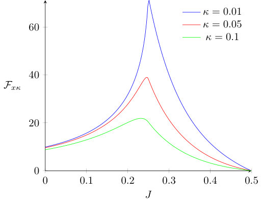 Figure 1
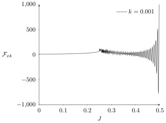 Figure 2
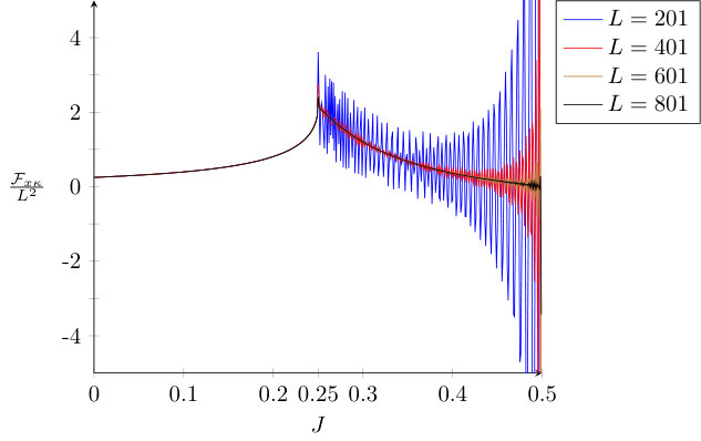 Figure 3
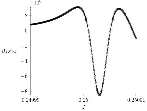 Figure 4
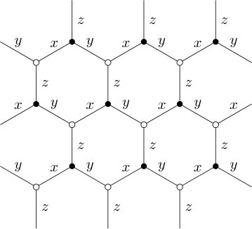 Figure 5
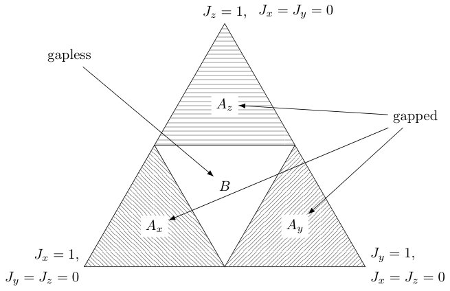 Figure 6
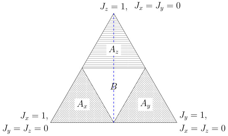 Figure 7
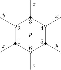 Figure 8
Peer Reviews
No public reviews on file for this paper yet. If you reviewed it on a platform where reviews are public (OpenReview, ICLR, NeurIPS, ICML), you can paste yours below so the community can read it here.
Videos
No videos yet. Explain this paper in a talk, walkthrough, or lecture? Add one.
On critical properties of Berry curvature in Kitaev Honeycomb model
Francesco Bascone1,2, Luca Leonforte3, Davide Valenti3,4, Bernardo Spagnolo3,5,6 and Angelo Carollo3,5
1Dipartimento di Fisica ”E. Pancini”, Università di Napoli Federico II, Complesso Universitario di Monte S. Angelo Edificio 6, via Cintia, 80126 Napoli, Italy
2Istituto Nazionale di Fisica Nucleare, Sezione di Napoli, Complesso Universitario di Monte S. Angelo Edificio 6, via Cintia, 80126 Napoli, Italy
3Dipartimento di Fisica e Chimica “Emilio Segré”, Group of Interdisciplinary Theoretical Physics, Università di Palermo, Viale delle Scienze, Edificio 18, I-90128 Palermo, Italy
4IBIM-CNR Istituto di Biomedicina ed Immunologia Molecolare “Alberto Monroy”, Via Ugo La Malfa 153, I-90146 Palermo, Italy
5Radiophysics Department, National Research Lobachevsky State University of Nizhni Novgorod, 23 Gagarin Avenue, Nizhni Novgorod 603950, Russia
6Istituto Nazionale di Fisica Nucleare, Sezione di Catania, Via S. Sofia 64, I-90123 Catania, Italy
Abstract
We analyse the Kitaev honeycomb model, by means of the Berry curvature with respect to Hamiltonian parameters. We concentrate on the ground-state vortex-free sector, which allows us to exploit an appropriate Fermionisation technique. The parameter space includes a time-reversal breaking term which provides an analytical headway to study the curvature in phases in which it would otherwise vanish. The curvature is then analysed in the limit in which the time-reversal-symmetry-breaking perturbation vanishes. This provides remarkable information about the topological phase transitions of the model. A non-critical behaviour is found in the Berry curvature itself, which shows a distinctive behaviour in the different phases. The analysis of the first derivative shows a critical behaviour around the transition point.
††: \JSTAT
Keywords Topological Phases of Matter, Quantum Phase Transitions, Anyons and Fractional statistical models.
1 Introduction
Topological phase transitions (TPTs) have emerged as a new paradigm, since they do not fall under the Landau theory description, where phases are characterised by local order parameters and symmetry breaking occurring across criticalities. Topological phases indeed are identified in the bulk by topological invariants, i.e. quantities that only depend on the topology, that are constructed out of ground states properties [1, 2, 3, 4]. Topological systems have attracted intense interest because of their peculiar properties, such as topologically protected edge states [5] or exotic statistics excitations [6, 7, 8]. Moreover, new materials are discovered and experiments are performed in the direction of probing anyonic excitations, which have promising applications in many other areas such as quantum computing.
Most of the literature on TPTs concerns the zero temperature case, where the systems are described by pure states. Recently efforts were also made in the direction of a mixed state generalisation [9, 10, 11, 12, 13, 14, 15, 16, 17, 18, 19, 20, 21, 22], to account for the effect of temperature in systems at thermal equilibrium or in out-of-equilibrium scenarios [23, 24, 25, 26, 27, 28, 29, Spagnolo2016, 30].
Moreover, much effort has been done to study the fault-tolerant quantum computation via topology[8, 31, 32, 33]. In this context a main role is played by the Kitaev honeycomb model [34], which possesses a rich phase structure allowing for the presence of both Abelian and non-Abelian anyonic excitations. Non-Abelian anyons are in fact a crucial building block of topological quantum computing since one can perform unitary operations by braiding these excitations. The model was also analysed at finite temperature in Ref. [9] by using the mean Uhlmann curvature as a main tool. The analysis of finite temperature phase transitions indeed is particularly important in the quantum computing framework since it could help to understand how the topological concepts can be used at finite temperature and therefore better exploited in applications. The honeycomb model under consideration shows a phase diagram containing gapped and gapless phases. In particular, we introduce a time-reversal symmetry breaking term, such that the system belongs to the symmetry-protected class . The latter is characterised by a charge conjugation symmetry and by the absence of time-reversal and chiral symmetries [4]. Such an external perturbation allows for the existence of non-Abelian excitations and opens a gap in an otherwise gapless phase. The main motivation of this work however is to introduce such a perturbation to analyse the Berry curvature of the system. Accordingly, one of the main results of this paper is the analysis of the Berry curvature of the Kitaev honeycomb model, both numerically and analytically, carried out in the presence of a time-reversal-symmetry-breaking perturbation. In particular, we will focus on the non-analytical behaviour of the curvature in the limit in which the above perturbation tends to zero. This procedure becomes necessary since the curvature is trivial in the vanishing perturbation case, which does not allow to gain any information on phase transitions eventually present in the system. On the contrary, extending the parameter manifold by including such a perturbation and then letting the coupling go to zero allow to recover information about the topological phase transitions.
The paper is organised as follows. In section 2 we discuss the spin honeycomb model and its phase diagram, by employing the Fermionisation procedure introduced in Ref. [35], which has the advantage to provide a closed form of the ground state in a BCS form. This technique permits to consider the system as a two-band p-wave topological superconductor, allowing for more convenient calculations. In section 3 we carry out the calculation of the Berry curvature for the ground state, which is unique in the planar geometry. In particular, we calculate and analyse the Berry curvature and its derivative in the vanishing external perturbation limit, both analytically and numerically. The analytic estimation is performed by expanding the curvature around the Dirac points. Section 4 contains the concluding remarks.
2 Honeycomb model
In this paper we consider the Kitaev honeycomb model [34], which consists of spin- particles arranged on the vertices of a honeycomb lattice. This model can support a rich variety of topological behaviors, depending on the values of its couplings.
The Hamiltonian of the system can be written as follows
[TABLE]
with denoting directional spin interaction between , sites connected by -link (see Fig. 1). are the dimensionless coupling coefficients of the two-body interaction and the are the Pauli operators.
Products of the operators can be used to construct loops on the lattice and any loop constructed in this way commutes with all other loops and with the Hamiltonian. In particular, the shortest loop symmetries are the plaquette operators
[TABLE]
where is a plaquette index, and is the number of plaquettes (Fig. 2).
These operators, which represent loops around single hexagons, commute with each other and with the Hamiltonian. Therefore they are integrals of motion and the Hilbert space of the system can be divided into sectors, each of which is eigenspace of a different . Each loop operator has eigenvalues , and plaquettes with are said to carry a vortex. Therefore, each sector corresponds to a particular choice of the string of eigenvalues over all the plaquettes .
In this way, the Hamiltonian can be decomposed as a direct sum over all the configurations:
[TABLE]
Thus, one needs to find the eigenvalues of the Hamiltonian restricted to a particular sector, and there are several ways to exactly solve this problem. We use a Fermionisation approach first developed in Refs. [35, 36]. This technique consists of a Jordan-Wigner (JW) Fermionisation, mapping “hard-core” bosons operators to Fermionic operators through string operators. This procedure allows for an explicit construction of the eigenstates of the system, leading to a closed form of the groundstate.
A theorem by Lieb [37] shows that the ground state of the system must lie in the vortex-free sector, while its degeneracy and form depend on the manifold considered. By focusing on the vortex-free sector, in a planar lattice geometry, we can take advantage of the translational symmetry and use the Fourier transform to derive the energy spectrum. By performing the JW transformation, we get the following Bogoulibov-deGennes (BdG)-like Hamiltonian:
[TABLE]
where,
[TABLE]
with
[TABLE]
Here we use a Cartesian basis where .
Thus, the Kitaev honeycomb model is mapped into a spinless Fermionic BdG Hamiltonian. The Hamiltonians can be diagonalised via Bogoliubov rotation of the mode operators, and the diagonalised Hamiltonian becomes
[TABLE]
whose ground state has the BCS form
[TABLE]
From the dispersion relation
[TABLE]
it is possible to find out the phase diagram structure of the system.
Indeed it can be easily checked that the following triangular inequalities
[TABLE]
if satisfied, identify the gapless regions of the spectrum. In Fig. 3 we explicitly show the above triangular condition in the positive octant (). The graphical representation in the other octants can be easily derived by symmetry. The triangular region in the phase diagram determined by such triangular conditions is named gapless B phase, while the other three regions (equivalent to each other) are indicated as gapped A phases.
3 Berry curvature analysis in the limit
In this section, in view of extending the results obtained in Ref. [9], we calculate the Berry curvature, closely following the procedure used in that work. In particular, we focus on the vertex-free configuration in a planar geometry, to take into account only a single ground state and therefore to get an Abelian Berry curvature. Note that in general for the current analysis it is not necessary to embed the system on a torus.
The Hamiltonian in Eq. (5) can be rewritten explicitly as
[TABLE]
where , and are the Pauli matrices. In this form, the spectral Berry curvature can be easily computed by means of the relation
[TABLE]
where and .
It is straightforward to check that this curvature appears to be zero everywhere. This can be deduced as a result of time-reversal (TR) and parity (P) symmetries of the model. Namely, one can note that the vector and all its derivatives are entirely contained in the plane.
As discussed in introduction, adding a TR and/or P symmetry-breaking term in the Hamiltonian, for instance by means of an external magnetic field, results in a gap opening in the phase. This condition allows for the existence of non-Abelian anyonic excitations. Explicitly, one can add a three-body interaction term of the form [38]
[TABLE]
where is the three-body external coupling, playing the role of an ”effective magnetic field”.
The Hamiltonian in Eq. (5) remains of the same form, provided that a real part is added to , that is , with
[TABLE]
The diagonalised form of this Hamiltonian is then exactly the same as in Eq.(7), but with
[TABLE]
We can still write in the form of Eq.(11), but with a slightly different vector , and calculate again the spectral curvature. Of course, one should extend the -dimensional parameter manifold to a -dimensional one to include the extra parameter .
We find that the only non-vanishing components of the curvature in Eq.(12) are the , , which are explicitly given by
[TABLE]
In order to obtain the total curvature, the spectral curvature needs to be summed over all quasi-momenta q (or, in the thermodynamic limit, integrating over ).
Without loss of generality, we choose the octant with . The three gapped phases correspond to the region in the parameter space. The phase is instead realised by the conditions (10). The four phases are separated by quantum phase transition lines on which one of the is equal to the sum of the other two (see Fig. 3). A TR-P breaking perturbation (for instance the term in Eq. (13) with ) ) opens a gap in the otherwise gapless phase . This would make both the s and the phases gapped, but still with different properties: indeed, phases host Abelian excitations, whereas the low energy excitation of the phase satisfy non-Abelian anyonic statistics. Notice that, in the chosen octant, the two phases are separated by the plane , and independently of the phase we are in, the couplings have to satisfy such a normalisation condition. To explore the behaviour of the Berry curvature in the different phases and in particular on the transition lines between them, we can choose to study, without loss of generality, the system along the line, cutting vertically the triangle diagram (blue dashed line in Fig. 4).
This choice of cut line allows one to explore the dependence of the curvature in the and phases on , with a special focus on the critical line at . Under these conditions we can use and, because of the normalisation relation , the curvature components are expressed as functions of a single parameter along this line (the transition at is realised at ).
Along this evolution line, the terms appearing in the expressions for the curvature components can be simplified as follows:
[TABLE]
so that the Berry curvature components in the thermodynamic limit have the form
[TABLE]
with
[TABLE]
It is easy to see that only one of the above expressions is independent since and . This means that we can limit our analysis just to the component. As it is discussed in [9], this is a consequence of the specific symmetry of the chosen cut-line.
The numerical result of the integration along the line with for different values of is shown in Fig. (5). It is interesting to note that the function is peaked close to the transition line, at , while it is regular enough over the whole region . For we can expect that eventual criticalities may not be evidenced by the Berry curvature, while they are surely identified by the Chern number.
It is also worth noting that the vertical line in the phase diagram (see Fig. 4) is travelled downward, so that the phase is covered for while the phase is covered for .
The Berry curvature peak gets higher as decreases to zero. This can be explained on account of the inverse dependence of the Berry curvature on the gap, which, in turn, tightens as decreases. To analyse the case, we study the Berry curvature analytically, by estimating the integrals around the Dirac points. This approach is justified by the fact that the dominant contribution to the Berry curvature comes from the regions close to the Dirac points.
This analytical approximation is validated by a numerical analysis performed for small enough values of , yet large enough to avoid numerical instabilities.
The analytical approach entails finding the minima of the energy spectrum around which the integrand in Eq. (17) is expanded in series (we consider again only the component). The position of the minima crucially depends on the phases of the model, i.e. whether the coupling is larger or smaller than the critical value . We distinguish the expansion in two separate cases. From the analysis of the function in the region, it follows that two minima are found for the following values of the momentum components
[TABLE]
By performing a second order expansion of the integrand function around these minima and using the eigenvalues of the Hessian matrix
[TABLE]
along the minimum eigendirections we are left to compute the following integral:
[TABLE]
with
[TABLE]
We also used the fact that the cross terms in the expansion are odd and they do not contribute in the symmetric integration region. The integration variables and are the eigencoordinates, i.e. the momentum variables in the basis where the Hessian is diagonal. The finite integration radius is taken to enclose the minima and its explicit value is not important for the estimate. It is not hard to see that the contribution coming from vanishes in the limit, while for the other two contributions we find, in the same limit,
[TABLE]
with . We note that in the limit the Berry curvature is finite, which is in agreement with the numerical analysis.
However, even if there is no criticality, the Berry curvature still gives information about the different phases of the system: it can be seen numerically that for very small values of , resembling the limit, very different behaviors are found below and above the transition line . Namely, rapid oscillations appear in the non-trivial phase similarly to the behavior found in Ref. [39] for the fidelity susceptibility, as shown in Fig. 6, explicitly revealing the two different topological phases.
Such oscillations however seems to be related to the finite system size used for numerical analysis. One can indeed observe that the height of the peaks increases with the system size.
Since the Berry curvature does not show any criticalities, it is relevant to analyse also its first derivative (w.r.t. the parameter ). This analysis allows to estimate the derivative of the curvature, providing the following result:
[TABLE]
which diverges to in the limit, indicating the presence of a criticality (it is worth reminding that at this stage we are only considering the region at the right of the transition point for : ). Now we extend this analysis to the left of the transition point. In the region the only minimum in the momentum space is the point , around which the curvature is expanded. Following the same procedure as before, we calculate the eigenvalues of the Hessian matrix in :
[TABLE]
where we use the condition , which is compatible since we are interested in the limit. Expanding up to the second order around we have
[TABLE]
while the second order expansion of the energy is given by
[TABLE]
Under a suitable rotation the Hessian becomes a diagonal matrix. By rewriting the above function with respect to the rotated variables, we obtain
[TABLE]
and
[TABLE]
In Eq. (26) we do not need to specify the value of since, under the symmetric integration domain, the mixed term coming from the numerator vanishes. Hence, we are left to compute the following integral:
[TABLE]
with
[TABLE]
The integral computation is straightforward, and leads to the following result for the Berry curvature estimation in the region in the limit:
[TABLE]
It is easy to see that the latter expression is finite in the limit. However, just as in the right limit case, we also analyse the first derivative behaviour. The expression for the derivative is the following:
[TABLE]
with
[TABLE]
[TABLE]
[TABLE]
[TABLE]
It can be seen that this derivative diverges to in the limit, in agreement with the numerical result (see Fig. (8)). We observe that the position of the criticality is not exactly at but slightly shifted on the right. This is due to the finite system size used in the numerical analysis. As expected, one can show that in the limit of size tending to infinity the criticality tends towards .
Therefore, the analysis of the Berry curvature at shows a critical behaviour, revealing a topological phase transition at . The ”detection” of this criticality would not be possible without the expansion procedure we carried out in the parameter space.
4 Conclusions
After briefly reviewing the Kitaev honeycomb model, we used a suitable Fermionisation technique to map our Hamiltonian to a BdG one, obtaining explicit relations for the relevant quantities we were interested in. In particular, we assumed a translationally symmetric condition, by considering the vortex-free sector of the model on an infinite plane. In Sec. 3 we have calculated the Berry curvature by assuming an expanded parameter manifold, which included an external effective magnetic field. This perturbation changes the class of the model from an intrinsic topological material to a symmetry protected one. This allowed to get an analytical headway for the calculation of the Berry curvature in the limit, in which the curvature would be otherwise identically zero. We estimated the Berry curvature in the limit by expanding around the relevant Dirac points. We found no criticalities, although this procedure provides information about the phase transitions of the system due to the appearance of rapid oscillations in the non-trivial phase. To better investigate the origin of these oscillations, we calculated the first derivative of the Berry curvature, which showed a divergence that clearly signals a phase transition. Therefore, the analysis of the Berry curvature in the limit shows a criticality in the transition line that was not possible to estimate without an appropriate expansion in the parameter space.
Acknowledgments
This work was supported by the Grant of the Government of the Russian Federation, contract No. 074-02-2018-330 (2). We acknowledge also partial support by Ministry of Education, University and Research of the Italian government.
The reference list from the paper itself. Each links out to its DOI / PubMed record.
- 1[1] Altland A and Zirnbauer M R 1997 Phys. Rev. B 55 1142–1161 ISSN 0163-1829 URL https://link.aps.org/doi/10.1103/Phys Rev B.55.1142
- 2[2] Schnyder A P, Ryu S, Furusaki A and Ludwig A W W 2008 Phys. Rev. B 78 195125 ISSN 1098-0121 URL https://link.aps.org/doi/10.1103/Phys Rev B.78.195125
- 3[3] Ryu S, Schnyder A P, Furusaki A and Ludwig A W W 2010 New J. Phys. 12 065010 ISSN 1367-2630 URL http://stacks.iop.org/1367-2630/12/i=6/a=065010?key=crossref.8100 f 885f 6d 94a 261914942850 e 92d 50
- 4[4] Chiu C K, Teo J C Y, Schnyder A P and Ryu S 2016 Rev. Mod. Phys. 88 035005 ISSN 0034-6861 URL https://link.aps.org/doi/10.1103/Rev Mod Phys.88.035005
- 5[5] Hatsugai Y 1993 Phys. Rev. Lett. 71 3697–3700 ISSN 0031-9007 URL https://link.aps.org/doi/10.1103/Phys Rev Lett.71.3697
- 6[6] Laughlin R B 1983 Phys. Rev. Lett. 50 1395–1398 ISSN 0031-9007 URL https://link.aps.org/doi/10.1103/Phys Rev Lett.50.1395
- 7[7] Arovas D P, Schrieffer J R and Wilczek F 1984 Fraction statistics and the Quantum Hall effect URL papers 2://publication/uuid/E 61AB 9D 9-FE 7B-4EA 4-9244-1147363676 D 5
- 8[8] Nayak C, Simon S H, Stern A, Freedman M and Das Sarma S 2008 Rev. Mod. Phys. 80 1083–1159 ISSN 0034-6861 URL https://link.aps.org/doi/10.1103/Rev Mod Phys.80.1083