TL;DR
SABER introduces a systems-based method for modeling, estimating, and reducing blur in X-ray images by combining multiple PSFs and applying deblurring algorithms, improving image clarity and contrast.
Contribution
The paper presents a novel systems approach to model and estimate the combined source and detector PSFs in X-ray imaging, enabling effective blur reduction.
Findings
Accurate estimation of source and detector PSFs from multiple radiographs.
Effective blur reduction using estimated PSFs through deblurring algorithms.
Improved image sharpness and contrast in X-ray radiographs.
Abstract
Blur in X-ray radiographs not only reduces the sharpness of image edges but also reduces the overall contrast. The effective blur in a radiograph is the combined effect of blur from multiple sources such as the detector panel, X-ray source spot, and system motion. In this paper, we use a systems approach to model the point spread function (PSF) of the effective radiographic blur as the convolution of multiple PSFs, where each PSF models one of the various sources of blur. In particular, we model the combined contribution of X-ray source and detector blurs while assuming negligible contribution from other forms of blur. Then, we present a numerical optimization algorithm for estimating the source and detector PSFs from multiple radiographs acquired at different X-ray source to object (SOD) and object to detector distances (ODD). Finally, we computationally reduce blur in radiographs…
Click any figure to enlarge with its caption.
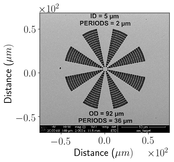 Figure 1
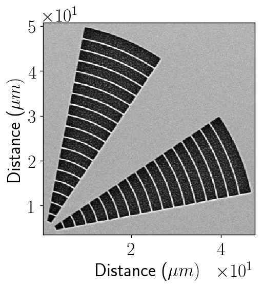 Figure 2
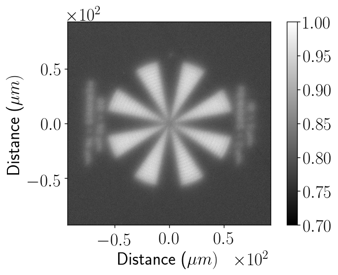 Figure 3
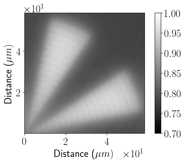 Figure 4
 Figure 5
 Figure 6
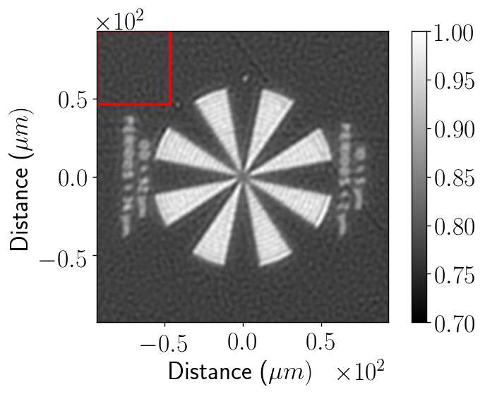 Figure 7
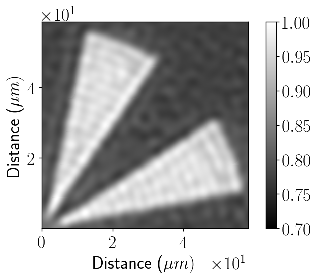 Figure 8
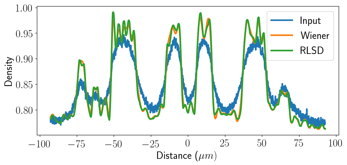 Figure 9
 Figure 10
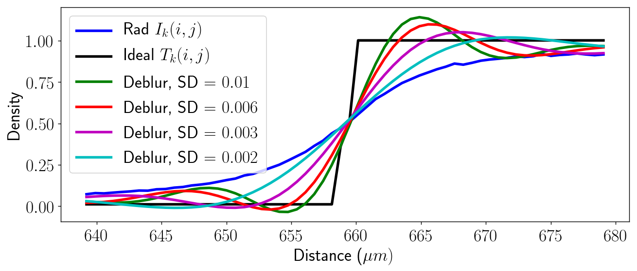 Figure 11
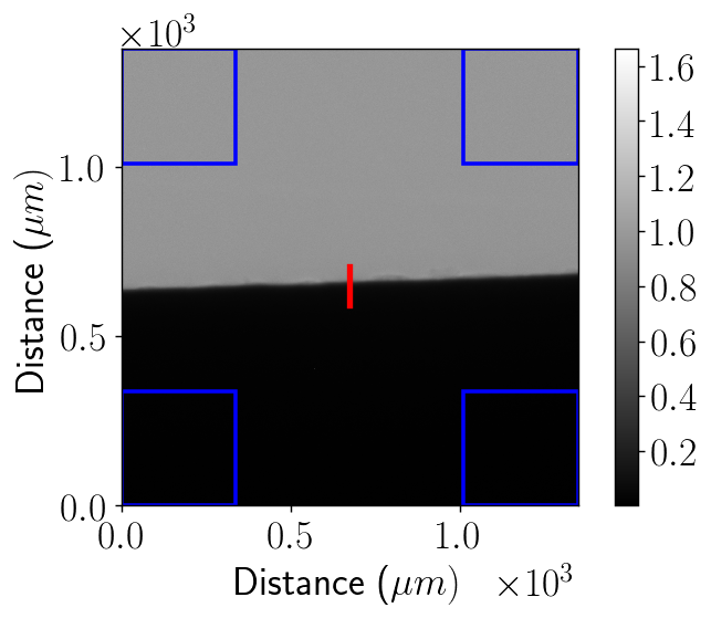 Figure 12
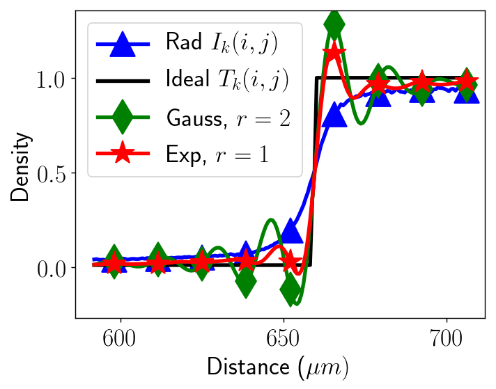 Figure 13
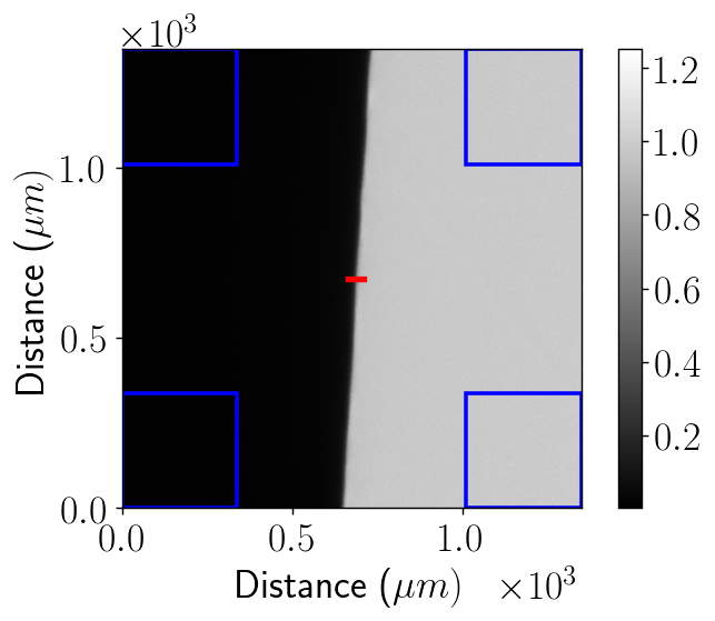 Figure 14
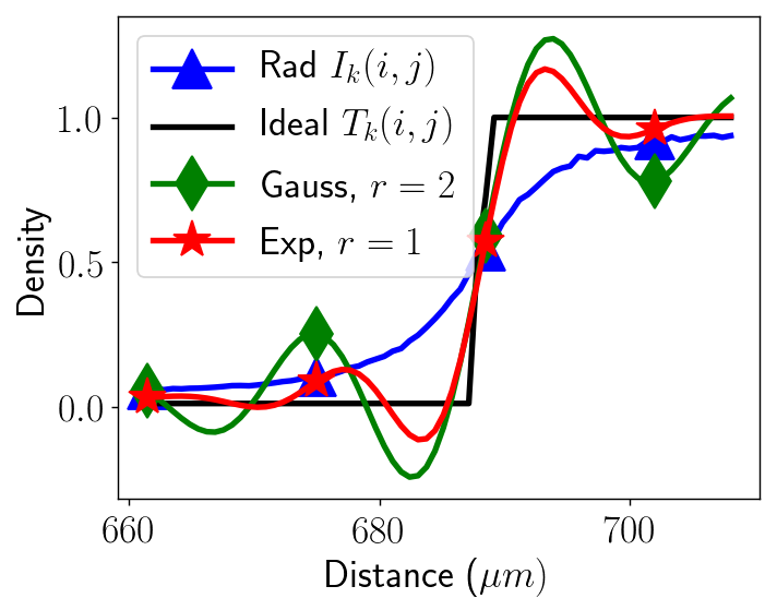 Figure 15
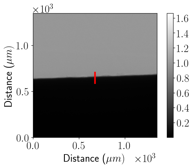 Figure 16
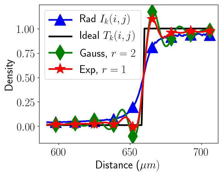 Figure 17
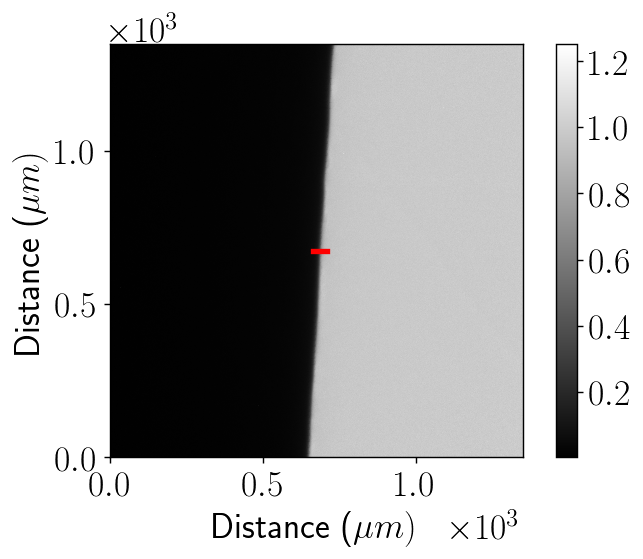 Figure 18
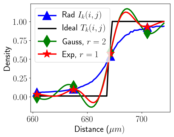 Figure 19
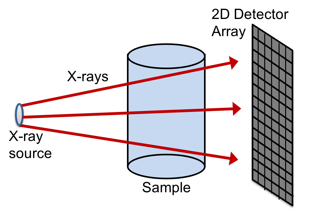 Figure 20
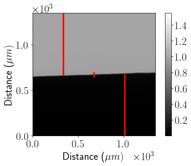 Figure 21
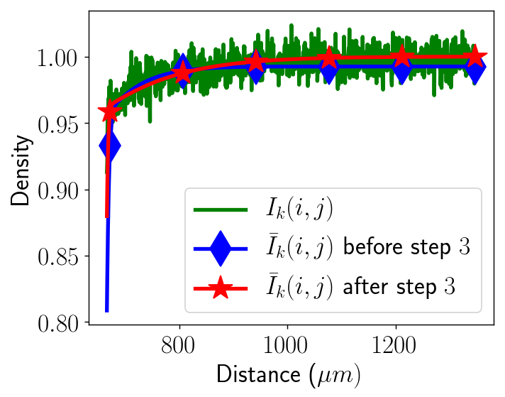 Figure 22
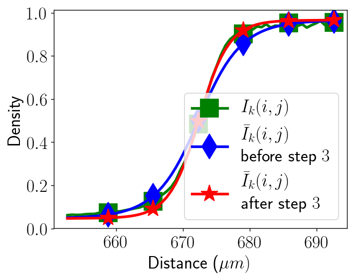 Figure 23
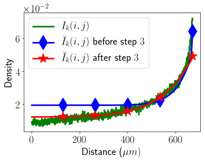 Figure 24
 Figure 25
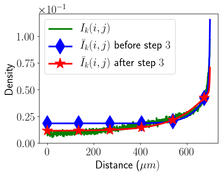 Figure 26
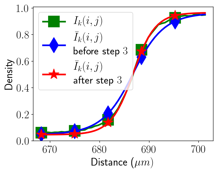 Figure 27
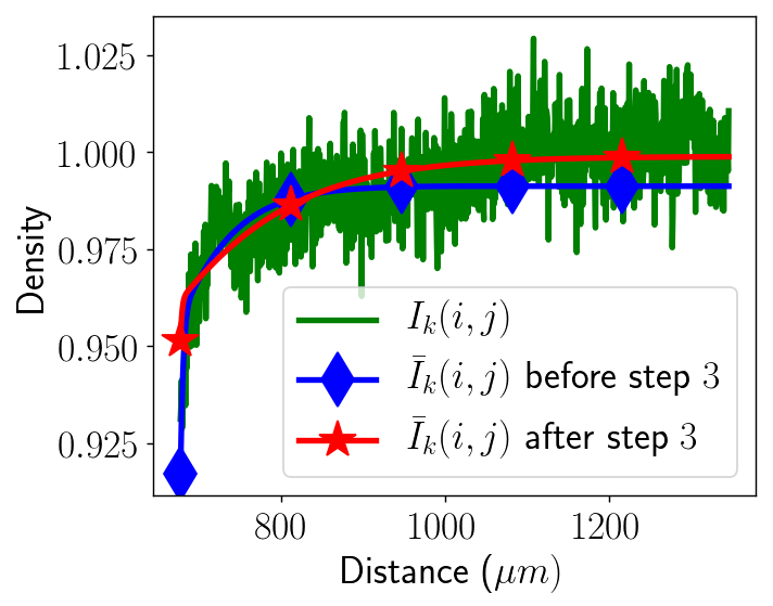 Figure 28
 Figure 29
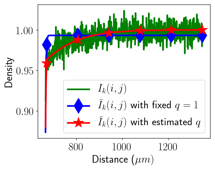 Figure 30
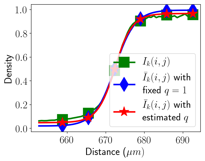 Figure 31
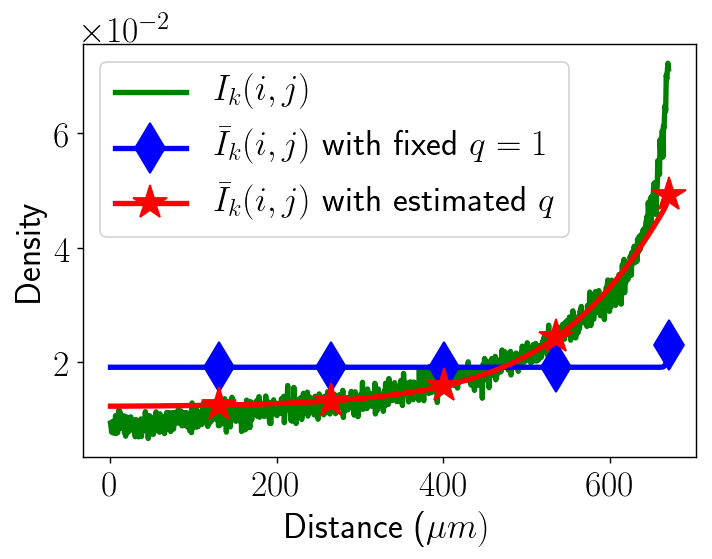 Figure 32
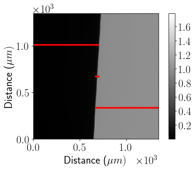 Figure 33
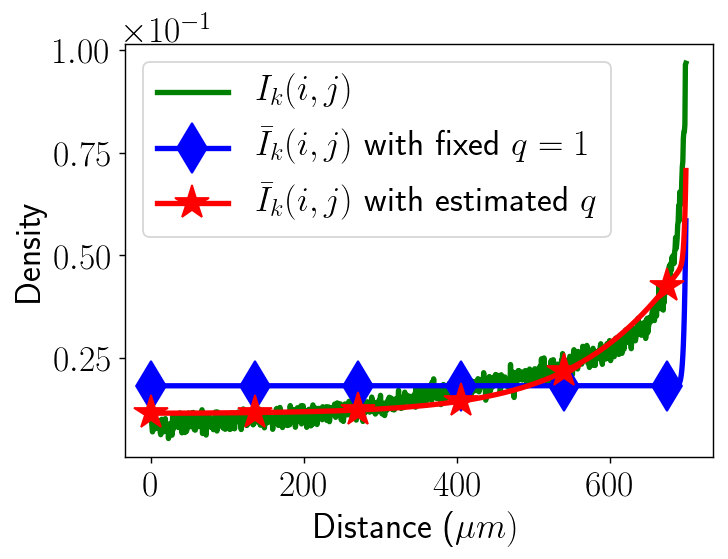 Figure 34
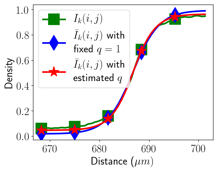 Figure 35
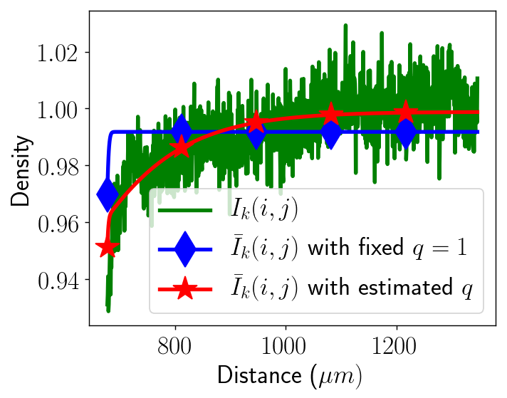 Figure 36
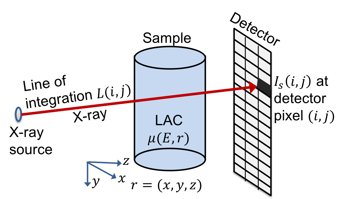 Figure 37
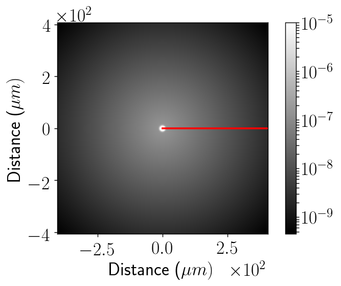 Figure 38
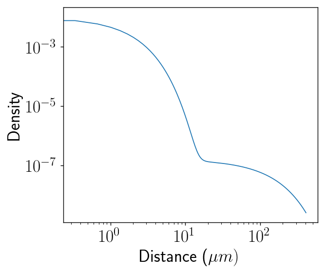 Figure 39
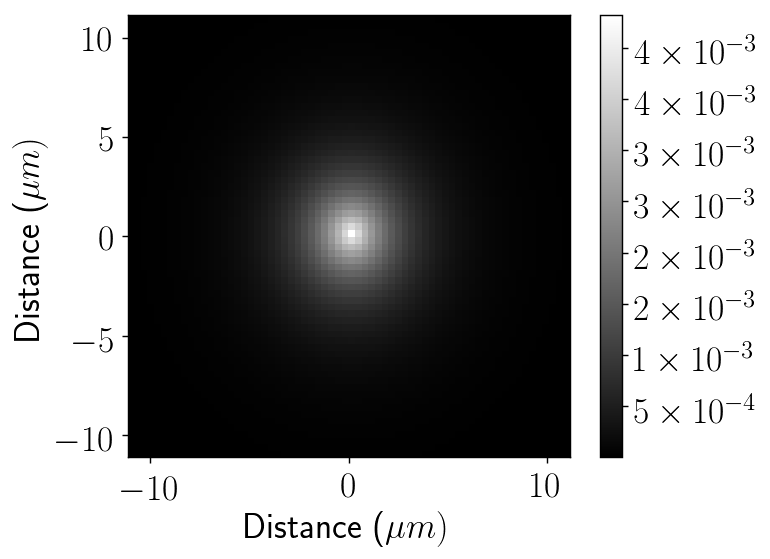 Figure 40
| horizontal | vertical | ||
| SOD () | SOD () | () | () |
| 12.0 | 13.0 | 3.2 | 3.6 |
| 24.8 | 24.8 | 3.6 | 3.9 |
| 37.5 | 37.5 | 4.5 | 4.6 |
| 50.3 | 50.3 | 6.9 | 6.9 |
| 65.3 | 60.0 | 13.0 | 25.9 |
| horizontal | vertical | |||
| SOD () | SOD () | () | () | |
| 12.0 | 13.0 | 12.6 | 130.6 | 0.89 |
| 24.8 | 24.8 | 5.7 | 134.9 | 0.91 |
| 37.5 | 37.5 | 3.4 | 158.3 | 0.92 |
| 50.3 | 50.3 | 2.3 | 127.0 | 0.92 |
| 65.3 | 60.0 | 1.9 | 118.3 | 0.93 |
| horizontal | vertical | |||||
| SOD () | SOD () | () | () | () | () | |
| 12.0,24.8 | 13.0,24.8 | 2.6 | 3.0 | 1.5 | 135.7 | 0.90 |
| 12.0,37.5 | 13.0,37.5 | 2.6 | 3.0 | 1.9 | 150.1 | 0.91 |
| 12.0,50.3 | 13.0,50.3 | 2.6 | 3.0 | 1.9 | 142.7 | 0.91 |
| 12.0,65.3 | 13.0,60.0 | 2.7 | 3.1 | 1.8 | 148.2 | 0.92 |
| 24.8,37.5 | 24.8,37.5 | 2.7 | 3.0 | 1.9 | 138.0 | 0.91 |
| 24.8,50.3 | 24.8,50.3 | 2.7 | 3.0 | 1.9 | 126.7 | 0.92 |
| 24.8,65.3 | 24.8,60.0 | 2.7 | 3.1 | 1.8 | 126.8 | 0.92 |
| 37.5,50.3 | 37.5,50.3 | 2.9 | 2.9 | 1.9 | 134.7 | 0.92 |
| 37.5,65.3 | 37.5,60.0 | 2.9 | 3.1 | 1.9 | 134.9 | 0.93 |
| 50.3,65.3 | 50.3,60.0 | 2.9 | 2.9 | 1.9 | 119.7 | 0.93 |
| Mean | 2.7 | 3.0 | 1.8 | 135.7 | 0.92 |
| Std Dev | 0.12 | 0.07 | 0.11 | 9.2 | 0.01 |
| 4.4% | 2.3% | 6.1% | 6.8% | 1.09% |
| () | () | () | () | ||
| Before step (3) | 4.5 | 4.6 | 2.3 | 67.6 | 0.92 |
| After step (3) | 2.9 | 2.9 | 1.9 | 134.7 | 0.92 |
| Prediction | Deblur, SD = | Deblur , SD = | ||||||
| PSF | Source | Detector | / | / | / | / | / | / |
| Model | Blur | Blur | ||||||
| Gaussian | Yes | No | 0.0172 | 0.0157 | 0.0717 | 0.0192 | 0.0516 | 0.0172 |
| Exponential | Yes | No | 0.0164 | 0.0157 | 0.0387 | 0.0188 | 0.0338 | 0.0171 |
| Gaussian | No | Yes | 0.0228 | 0.0086 | 0.0309 | 0.0327 | 0.0296 | 0.0226 |
| Exponential | No | Yes | 0.0223 | 0.0083 | 0.0322 | 0.0161 | 0.0309 | 0.0132 |
| Gaussian | Yes | Yes | 0.0149 | 0.0081 | 0.0367 | 0.0168 | 0.0289 | 0.0126 |
| Exponential | Yes | Yes | 0.0147 | 0.0078 | 0.0264 | 0.0139 | 0.0243 | 0.0111 |
| Horizontal | Vertical | Deblur | Deblur |
| SOD () | SOD () | SD = | SD = |
| 12.0,37.5 | 13.0,37.5 | 0.0242 | 0.0222 |
| 12.0,50.3 | 13.0,50.3 | 0.0246 | 0.0226 |
| 12.0,65.3 | 13.0,60.0 | 0.0241 | 0.0220 |
| 37.5,50.3 | 37.5,50.3 | 0.0264 | 0.0243 |
| 37.5,65.3 | 37.5,60.0 | 0.0258 | 0.0236 |
| 50.3,65.3 | 50.3,60.0 | 0.0262 | 0.0242 |
Peer Reviews
No public reviews on file for this paper yet. If you reviewed it on a platform where reviews are public (OpenReview, ICLR, NeurIPS, ICML), you can paste yours below so the community can read it here.
Code & Models
Videos
No videos yet. Explain this paper in a talk, walkthrough, or lecture? Add one.
SABER: A Systems Approach to Blur Estimation and Reduction in X-ray Imaging
K. Aditya Mohan, Robert M. Panas, and Jefferson A. Cuadra K. A. Mohan is with the Computational Engineering Division (CED) at Lawrence Livermore National Laboratory, Livermore, CA, 94551 USA. E-mails: [email protected], [email protected]. M. Panas and J. A. Cuadra are with the Materials Engineering Division (MED) at Lawrence Livermore National Laboratory, Livermore, CA, 94551 USA. 0000-0002-0921-6559
Abstract
Blur in X-ray radiographs not only reduces the sharpness of image edges but also reduces the overall contrast. The effective blur in a radiograph is the combined effect of blur from multiple sources such as the detector panel, X-ray source spot, and system motion. In this paper, we use a systems approach to model the point spread function (PSF) of the effective radiographic blur as the convolution of multiple PSFs, where each PSF models one of the various sources of blur. In particular, we model the combined contribution of X-ray source and detector blurs while assuming negligible contribution from other forms of blur. Then, we present a numerical optimization algorithm for estimating the source and detector PSFs from multiple radiographs acquired at different X-ray source to object (SOD) and object to detector distances (ODD). Finally, we computationally reduce blur in radiographs using deblurring algorithms that use the estimated PSFs from the previous step. Our approach to estimate and reduce blur is called SABER, which is an acronym for systems approach to blur estimation and reduction.
Index Terms:
Blur, deblur, optimization, algorithm, radiography, tomography, source blur, detector blur, motion blur, deconvolution, model estimation, high resolution.
I Introduction
X-ray imaging systems are widely used for 2D and 3D non-destructive characterization and visualization of a wide range of objects. The ability of X-rays to penetrate deep inside a material makes it a useful tool to visualize the interior morphology of objects. X-ray imaging is very popular in applications such as industrial imaging [1, 2, 3, 4], medical diagnosis [5, 6], and border security [4, 7, 8, 9]. A schematic representation of a typical cone-beam X-ray imaging system is shown in Fig. 1. Here, an object is exposed to a diverging beam of X-ray radiation that is generated by a X-ray source. The X-rays get attenuated as they propagate through the object and an image of the attenuated X-ray intensity is recorded by a detector consisting of a flat-panel 2D array of sensors.
The resolution of an X-ray image, also called a radiograph, is limited by several factors. The detector used to record the radiograph imposes a fundamental limit on the resolution by fixing the smallest pixel size. Also, detector cross-talk where energy from one sensor pixel leaks into its neighboring sensor pixels [10] causes blur and contrast reduction. Furthermore, the finite non-zero area of the X-ray source aperture manifests as additional blur in the radiograph [11, 12]. Other causes of blur include motion or vibrations in the sample stage or the imaging equipment. Blur is a major detriment in dimensional metrology applications where it is critical to accurately estimate the relative physical distances between image features. In medical applications, blur hinders the ability to resolve small features such as tumors that may only be a few pixels in size [13]. Hence, mitigating blur is vital to many applications especially when quantitative accuracy is important.
In order to quantify radiographic blur, we use a parametric mathematical model to describe the blurring process. Several papers address the problem of mathematically modeling numerous types of blur such as X-ray source spot blur, detector cross-talk, motion blur, and scatter [14, 15, 11]. A popular strategy is to model blur as a convolution operation with a certain point spread function (PSF). Here, the PSF used to model blur is derived using either simulation [16] or data-driven approaches [17, 18, 19, 20, 21, 22, 23]. Simulation of PSF relies on precise engineering knowledge of the relevant imaging equipment that may not always be available. Alternatively, data-driven approaches estimate PSF directly from radiographs of known well characterized objects.
Data-driven approaches to blur estimation relies on calculation of the PSF from radiographs of an object with known composition and shape such as a rollbar, slit, pinhole, or other test objects [17, 18, 19, 20, 21]. However, these methods only estimate one PSF that either models the X-ray source blur, the detector blur, or the total effective blur. They do not address the problem of disentangling and estimating the PSFs of all the different types of blur that simultaneously affect a radiograph. The magnitude of each blur varies depending on the relative placement of the X-ray source, object, and detector. The ability to estimate each individual blur PSF will allow us to predict the radiograph blur for any spatial configuration of X-ray source, object, and detector by appropriately recombining the estimated blur PSFs.
Blur in X-ray radiographs can be reduced either by hardware upgrades or using computational algorithms to reduce blur after the experiment. The former approach may not always be feasible due to cost or physical constraints. Alternatively, deblurring algorithms are a cheaper solution to computationally reduce blur in radiographs. The estimated blur PSFs can be used in a wide variety of deblurring algorithms [24, 25, 26, 27, 28, 29] to reduce blur in radiographs.
In this paper, we present an extensible framework called systems approach to blur estimation and reduction (SABER) for modeling, characterizing, and reducing the various types of blur in a X-ray imaging system. We apply a systems approach to model blur by expressing the PSF of the effective blur in a radiograph as the convolution of multiple blur PSFs with varying origins. Then, we present a numerical optimization algorithm to disentangle and estimate the individual blur PSFs from radiographs of a Tungsten plate rollbar. In particular, we focus on the simultaneous estimation of the X-ray source and detector PSFs while assuming negligible motion blur and scatter. Preliminary results using this approach was previously published as an extended abstract [12]. Software that implements SABER is freely available in the form of a open-source python package called pysaber that is documented at the link https://pysaber.readthedocs.io/.
In section II, we present the underlying principles and mathematics of X-ray imaging. We formulate our blur model in section III and estimate its parameters using an optimization algorithm in section IV. In section V, we present two approaches to deblurring radiographs. Finally, results using real experimental data from a Zeiss Xradia Versa X-ray imaging scanner are presented in section VI.
II Background
Beer’s law [30] is used to express the magnitude of X-ray attenuation within an object in terms of its thickness and material properties. X-ray attenuation is dependent on a material property called linear attenuation coefficient (LAC) which is a function of the object’s chemical composition, density, and X-ray energy. At detector pixel shown in Fig. 2, according to Beer’s law, the ratio of the X-ray measurement with the object, , and the X-ray measurement without the object, , is given by,
[TABLE]
where is the LAC of the object at X-ray energy and spatial location , is the line along which is integrated, and is the X-ray spectral density such that [4]. We will call the expression on the right side of the equality in equation (1) as the ideal transmission function , i.e.,
[TABLE]
The relation in equation (1) is valid in the absence of imaging non-idealities such as noise, blur, and scatter. Dark current is one such non-ideal characteristic where the detector measurements do not drop to zero when there is no X-ray radiation. To compensate for this effect, detector measurements are made without the X-ray beam and subtracted from measurements with the X-ray beam. Detector measurements are also corrupted by electronic noise and photon counting noise that are often modeled as additive Gaussian noise. Let denote the normalized measurement defined as the ratio of the dark noise corrected measurements with and without the object. If denotes the measurement at detector pixel without X-rays, then,
[TABLE]
where is Gaussian noise. In the next section, we will modify equation (3) to account for the effects of more non-idealities such as X-ray source blur and detector blur.
The term “radiograph” will henceforth be used to refer to the normalized radiograph i.e., over all pixel locations . Also, “bright field” is used to refer to and “dark field” is used to refer to .
III Formulation of Blur Model
The effect of various forms of blur on X-ray radiographs is modeled as a linear space-invariant phenomenon. The blur model expresses the radiograph as the convolution of a transmission function with multiple two dimensional PSFs each of which models a different form of blur. In the absence of non-idealities such as scatter or temporal drift in values of and , the transmission function is equal to the ideal transmission function given in equation (2).
First, we will consider the effect of blur due to X-ray source, detector, and system motion [31]. The size of the source and motion PSFs are a function of the X-ray source to object distance (SOD) and object to detector distance (ODD). Since detector blur is due to cross-talk between detector pixels, it does not vary with SOD and ODD. Let and denote the PSFs of the X-ray source blur and motion blur respectively on the detector plane at a SOD of and ODD of . If is the radiograph and is the transmission function at a SOD of and ODD of , then,
[TABLE]
where denotes 2D convolution (Fig. 3). Based on the analysis in [32, 33, 34], we will ignore the effect of motion PSF since its full width half maximum (FWHM) was determined to be much smaller than our detector pixel width. Thus, our goal is to estimate the PSFs of X-ray source and detector blur given equation (4) and radiographs at various SOD and ODD.
III-A Transmission Function
Simultaneous estimation of the transmission function, , and the blur PSFs, and , is an ill-posed problem. Hence, we scan a object with known dimensions and chemical composition. Since our object is known, we can compute the ideal transmission function for each scan (indexed by ) using equation (2). The transmission function is then modeled as an affine transformation of the ideal transmission function such that
[TABLE]
where and are scalars. The parameters and are used to compensate for uniform shifts in the measured X-ray intensity due to non-idealities such as drift in the values of and over time, inaccuracies in the calculation of , and low-frequency effects such as scatter. Temporal drifts in and can occur if there is any change in dark current or X-ray source intensity.
III-A1 Calibration Data
For our experiments, we fabricated a Tungsten plate with a sharp edge and uniform thickness that is sufficient to block all incoming X-rays (Fig. 4). The plate is then exposed to X-rays such that the sharp edge passes close to the center of the radiograph as shown in Fig. 5 (a). The plane of the Tungsten plate is aligned such that it is perpendicular to the direction of X-ray propagation. Since perfect alignment is very challenging, the sharp edges are rolled [19] to one meter radius of curvature, which permits alignment errors of up to one degree. Fig. 5 (b) shows the ideal transmission function for the radiograph in Fig. 5 (a). The procedure used to compute the ideal transmission function is presented in Appendix A.
III-A2 Initialization of and
Due to scatter and variations in and , is not the same as . The values of and that determine the relation between and in equation (5) are jointly estimated during the blur estimation procedure that will be presented in the next section. However, to aid this procedure, we have to supply initial estimates for that are determined by finding the best values for that solve the following over-determined set of linear equations,
[TABLE]
Here, is the weight term that is [math] for pixels that are close to the boundaries of the image and elsewhere (Fig. (5) (c)). The padded region of is also excluded from consideration during parameter estimation (Fig. (5) (d)). Equation (6) is solved using RANSAC regression [35, 36]. We used the scikit-learn [36] implementation of RANSAC111RANSAC Parameters: Minimum number of randomly chosen samples was . For a data sample to be classified as an inlier, the maximum residual threshold was . in this paper.
III-B Source Blur
The PSF of source blur is mathematically modeled using a 2D density function. This function is parameterized by two scale parameters and that are a measure of the spatial width of the PSF along the axis and axis in the plane of the X-ray source. If denotes the width of each pixel, the PSF of source blur in the plane of the X-ray source is modeled as,
[TABLE]
where and is the normalizing constant given by,
[TABLE]
The constant ensures that sums to one when summed over all . In equation (7), a Gaussian density function is obtained by setting and an exponential density function is obtained when . The scale parameters are related to the full width half maximums (FWHM) along the axis as and along the axis as . By definition, FWHM is the distance between two points along the axis where the PSF drops to half of its maximum value and FWHM is the corresponding distance along the axis.
At the detector plane, the FWHM of source blur is scaled by a factor of ODD/SOD. The change in FWHM of source blur with varying ODD and SOD is depicted in Fig. 6. For the radiograph, the PSF of source blur on the detector plane is given by,
[TABLE]
where is the normalizing constant given by,
[TABLE]
III-C Detector Blur
The detector blur is modeled using a mixture of two density functions with scale parameters and . If denotes the PSF of detector blur, then,
[TABLE]
where is the mixture parameter and are normalizing constants such that
[TABLE]
Also, and are parameters that function as weights for the two density functions. The scale parameters are related to the FWHMs of the two exponential functions in equation (11) as and . A Gaussian mixture model for detector blur is obtained by setting and an exponential mixture model is obtained when .
In our experiments, we expect the detector PSF to be dominated by the first exponential with a large weight of and a very small FWHM that spans only a few pixels. The second exponential is expected to have a smaller weight of and a very large FWHM that spans several hundreds of pixels. Depending on the X-ray imaging system, the values for and may change but equation (11) is still expected to be a good model for detector PSF.
III-D Motion Blur
An additional source of blur is the relative motion of all components in the X-ray system. If these components move during the data acquisition period, then they will result in motion of the object’s image on the detector surface. Such motion will distribute the apparent location of an edge or feature over a range of locations, appearing to blur it in a manner that can be captured with a motion PSF that is convolved with the image. The system motion is calculated via a geometric analysis of the relative locations of components, propagated to the detector screen. This is done using an uncertainty propagation model presented in [32, 33, 34]. Motion blur is denoted by and is typically modeled as a Gaussian density function. This form of blur also depends on the relative positions of X-ray source, object, and detector. However, we will effectively ignore the motion PSF by modeling it as a delta function since its FWHM was determined to be much smaller than the detector pixel width in our experiments. Thus, the form of is given by,
[TABLE]
IV Estimation of Blur Model
Blur model estimation is the process of estimating all the parameters and of the PSFs given known values for and in equations (4) and (5). We will only estimate and in equation (4) since is assumed to be a constant delta function. By constraining to take the shape of the density function in equation (7) and to take the shape of the mixture density function in equation (11), blur estimation reduces to the problem of estimating the parameters , , , , and . For every radiograph, the parameters and in equation (5) are also treated as unknowns and jointly estimated along with the PSF parameters.
Note that the form of source PSF as evaluated on the detector plane given by equation (9) depends on the ratio of the object to detector distance and the source to object distance . Thus, while the amount of source blur in the radiograph is a function of and , the detector blur does not change with and . To estimate both source and detector PSF parameters, it is necessary to acquire radiographs at a minimum of two different values of . Also, since the source PSF has two scale parameters modeling the width along axis and axis, we need radiographs for cases when the Tungsten edge is horizontal and vertical.
We use numerical optimization to estimate all blur and transmission parameters given radiographs at different values of ODD and SOD. The parameters are estimated by solving,
[TABLE]
[TABLE]
where and is the total number of radiographs. The parameters , , , , , , and are the estimated values of , , , , , , and respectively. The lower bound of for ensures that the first exponential in equation (11) is chosen to have the largest weight.
We solve the minimization problem in equation (15) using the L-BFGS-B algorithm [37]. L-BFGS-B is a quasi-Newton method for solving optimization problems and requires information of the gradient of the objective function, , with respect to all the variables being optimized. It also supports bound constraints on each of the variables that are optimized. However, since the optimization problem in equation (15) is non-convex, the optimized variables may be stuck in a local minima or a saddle point. Thus, good initialization of each variable is necessary to ensure reliable convergence to a solution that best fits the measured radiographs. Our approach to solving equation (15) is outlined in algorithm 1. We use the L-BFGS-B implementation in the python package scipy [38, 39]. The gradients that must be supplied to the L-BFGS-B algorithm are derived in Appendix B.
In algorithm 1, steps and are used to produce good initial estimates of the source and detector PSF parameters for initializing the optimization in step . In step , only source PSF parameters are estimated from half of all radiographs with the highest where source blur is significant if not dominant. In step , only detector PSF parameters are estimated from half of all radiographs with the lowest where detector blur is significant if not dominant. In step , all parameters from the source PSF, detector PSF, and transmission function are jointly optimized to arrive at the final estimates.
V Deblurring Algorithms
Deblurring is the process of reducing blur in radiographs using computational algorithms. We focus on using Wiener filter [25, 28] and regularized least squares deconvolution [27, 26, 28] for deblurring radiographs. These algorithms take as input the convolution of all PSFs given by,
[TABLE]
which is a function of the source to object distance and object to detector distance of the input radiograph . In equation (20), and are obtained by substituting the estimated values and from step 3 of algorithm 1 in equations (9) and (11). The PSF is assumed to be a discrete delta function (equation (14)) since FWHM of motion blur was determined to be much smaller than the pixel width using the analysis in [32, 33, 34].
V-A Wiener Filter
Wiener filter [25, 28] reduces blur by deconvolving the convolution of all PSFs, in equation (20), from the blurred radiograph . Deconvolution is implemented in Fourier space by dividing the Fourier transform of the radiograph with the Fourier transform of the PSFs. To reduce noise, regularization is used to enforce smoothness. We use the function skimage.restoration.wiener in the python package scikit-image [40] that implements the method in [25].
V-B Regularized Least Squares Deconvolution (RLSD)
In RLSD [27, 41, 28, 26], we solve the following optimization problem to deblur a radiograph ,
[TABLE]
where is the deblurred radiograph, is the regularization parameter, and is the set of all pairs of neighboring pixel indices i.e., if pixel lies within a neighborhood of pixel . The regularization weight parameter is inversely proportional to the distance between neighboring pixels and normalized such that , where is the set of all voxel indices that are neighbors to voxel index . For simplicity, the weight parameter is chosen to be for all in our experiments. Ideally, should be set such that it is inversely proportional to the variance of noise in .
The regularization function in equation (21) enforces smoothness in by penalizing the difference in values between neighboring pixels [41, 42]. The optimization problem in equation (21) is solved using the L-BFGS-B algorithm [37].
VI Results
In this section, we will estimate the blur model for a Zeiss Xradia 510 Versa X-ray imaging system. We will compare the efficacy of our blur model against conventional approaches using quantitative metrics. After estimating the blur model, we use Wiener filtering and RLSD (described in section V) to deblur radiographs.
The Versa is a commercial micro-CT system that consists of a transmissive X-ray tube with a Tungsten target anode that exhibits bremsstrahlung X-ray spectral characteristics. The accelerating voltage was selected to be and the tube current was . This resulted in an average flux of . The detector consists of an optically coupled Thallium-doped Cesium Iodide scintillator and a CCD with a pixel width, -bit depth, and a maximum dark current noise of about . Bright field images (radiographs without object) and dark field images (radiographs with X-rays off) were acquired to appropriately normalize each radiograph image of the object using equation (3). All radiographs were acquired using a magnification lens resulting in an effective pixel width of .
VI-A Blur PSF Parameter Estimation
Radiographs of a Tungsten plate rollbar are used to estimate the blur model parameters , and by solving the optimization problem in equation (15). The source to detector distance (SDD) for all radiographs was fixed at . First, the Tungsten plate edge is oriented in the vertical direction (Fig. 5 (a)) and radiographs are acquired at source to object distances (SOD) of , , , , and . Next, the edge is oriented in the horizontal direction and radiographs are acquired at SOD of , , , , and . Since SDD is , the object to detector distance (ODD) for each radiograph is given by (SOD). For each radiograph, the Tungsten plate is oriented such that its edge is slightly tilted away from the horizontal or vertical directions as shown in Fig. 5 (a). This is done to ensure that the Tungsten edge is never parallel to a row or column of detector pixels.
The traditional approach to estimating the PSF of X-ray source blur involves assuming that there is no detector blur. To demonstrate this approach, we estimate only the source and transmission parameters, and in equation (15), using a single set of horizontal and vertical edge radiographs while assuming there is no detector blur, which is enforced by setting
[TABLE]
The estimated values of X-ray source parameters for various source to object distances (SOD) are shown in Table I. The SOD of radiographs used during estimation are shown in the first two columns of Table I. Since FWHMs are more easily interpretable than scale parameters , we show the FWHMs instead of the scale parameters in the third and fourth columns of Table I. We see that the estimated values for the FWHMs consistently increase with increasing values of SOD in Table I since the source FWHMs were estimated while assuming there is no detector blur. Hence, the detector blur in the input radiographs get interpreted as X-ray source blur, which causes the FWHM of X-ray source blur to increase when SOD is increased.
The traditional approach to detector blur estimation involves assuming that there is no source blur. To evaluate this approach, we estimate only the detector and transmission parameters, and in equation (15), using a single set of horizontal and vertical edge radiographs while assuming there is no source blur, which is enforced by setting
[TABLE]
The estimated parameters of detector blur are shown in Table II. The SOD of radiographs used during estimation are shown in the first two columns of Table II. The estimated detector blur parameters are shown in the last three columns of Table II. In this case, we see that the estimated value for FWHM decreases with increasing SOD since we assumed that there is no X-ray source blur. Note that the first exponential with FWHM of in equation (11) is dominant since its weight given by is approximately in Table II. As SOD increases and ODD decreases, the FWHM of the source blur on the detector plane reduces. However, since source blur is interpreted as detector blur, the estimated FWHM also decreases as SOD is increased. In contrast, and do not seem to have a significant dependence on SOD.
To evaluate our proposed approach, we use horizontal edge radiographs at two SODs and vertical edge radiographs at two SODs to simultaneously estimate both source and detector blur parameters using algorithm 1. The estimated values of blur parameters after step 3 of algorithm 1 are shown in Table III. The SOD of radiographs used during estimation are shown in the first two columns of Table III. The estimated PSF parameters are shown in the last five columns of Table III. In this case, the estimation of X-ray source and detector parameters are stable without any noticeable dependence on SOD. Table IV shows the mean (row label Mean), standard deviation (row label Std Dev), and standard deviation as a percentage of the mean (row label ) of the estimated parameters in Table III computed across various SODs. From Tables III and IV, we can see that by simultaneously accounting for both the X-ray source and detector blur, we are able to perform stable estimation of all PSF parameters.
The source PSF as evaluated in the plane of the source and detector are shown in Fig. 7. The PSF is obtained by substituting the mean values of and shown in Table IV in equations (7) and (9). Since and are approximately the same, we can conclude that the source PSF is approximately circular in shape. Using the method in [21], the manufacturer of the X-ray system estimated the source PSF to have a FWHM of using calibration data at a SOD of and ODD of . For this case, the ratio ODD/SOD lies in between the data acquisition parameters of the second and third rows in Table I. Since the manufacturer’s estimate did not account for detector blur, their values are a good match with our estimates that also ignore detector blur.
The detector PSF is shown in Fig. 8 and is evaluated by substituting the mean values of , , and shown in Table IV in equation (11). Since the FWHM of the first exponential density in equation (11) with the high weight of is only a few pixels wide (pixel width being ), we can deduce that most of the detector blur is limited to only a few pixels. Alternatively, the large value of FWHM of the second exponential density with the smaller weight of suggests that there is significant leakage of electric charge all the way to the corners of the detector array.
Fig. 9 and Tables I, II, III, and V validate the necessity to simultaneously optimize the source blur, detector blur, and transmission function. While step 1 and step 2 of algorithm 1 independently estimate source and detector blur, step 3 estimates both forms of blur simultaneously. The estimated parameters before and after step (3) of algorithm 1 are shown in Table V. We can see that is significantly larger after step (3) than before step (3). This increase in is due to the simultaneous estimation of of the transmission function along with of detector blur in step 3 of algorithm 1. To obtain a better fit, the optimizer decreases , increases , which in turn allows for to increase. Since models the long tails of the detector PSF in equation (11), it is most sensitive to changes in and . Fig. 9 (b-d,f-h) shows line profile plots that compare the input radiograph with the prediction estimate before and after step 3 of algorithm 1. The improvement in fit after step (3) as demonstrated in Fig. 9 (c,g) is due to the change in parameters , , and . Similarly, the improvement in fit after step (3) in Fig. 9 (b,d,f,h) is due to the change in parameters , , and .
Fig. 9 (j-l) validates the necessity to model detector PSF as a mixture of two exponential density functions with FWHMs and (equation (11)). The first exponential function with FWHM and a high weight of ( in our experiments) models the blur close to the sharp edge that only span a few pixels as shown in Fig. 9 (k). The second exponential function with FWHM and a low weight of () models the slow variation in intensity values further away from the sharp edge as shown in Fig. 9 (j,l). From Fig. 9 (j,l), we can see that the detector PSF is not able to fit the slowly varying intensity that span several hundreds of pixels when is not estimated and fixed at . Fixing is equivalent to modeling detector PSF as consisting of only one exponential density function with a FWHM of .
VI-B Validating the Blur Model
The optimal choice of density function used to model the source blur in equation (7) and the detector blur in equation (11) is system dependent. In Table VI, we compare the performance of various choices of blur model using quantitative evaluation metrics. Horizontal and vertical edge radiographs at SODs of and were used when simultaneously estimating both source and detector blurs. When estimating only source blur, only radiographs at SOD of were used since source blur is dominant at the lower SOD. When estimating only detector blur, only radiographs at SOD of were used since detector blur is dominant at the higher SOD. The column of Table VI indicates whether the PSF model was chosen to be either Gaussian () or exponential (). The column indicates if source blur was modeled (marked as “Yes”) or ignored (marked as “No”). The column indicates if detector blur was modeled (marked as “Yes”) or ignored (marked as “No”). To determine the most appropriate blur model, we evaluate the blur prediction and deblurring performance on radiographs that were acquired at SOD values different than those used for blur estimation. Computation of the performance evaluation metric, root mean squared error (RMSE), in the , and columns is over both the horizontal and vertical edge radiographs at SOD of . Similarly, the RMSEs in the , and columns are computed over the horizontal edge radiograph at SOD of and vertical edge radiograph at SOD of .
The accuracy of blur prediction is quantified in the and columns under the header “Prediction ” by computing the RMSE between the measured radiographs and its predictions using the blur model. In order to compute , we must compute the transmission function by setting appropriate values for in equation (5) for radiographs that were not used during blur estimation. As an approximate solution to this problem, the and for horizontal/vertical edge prediction are chosen to be the average of the corresponding values for the horizontal/vertical edge transmission functions estimated during blur optimization. The lowest RMSE is obtained along the last row of Table VI, which corresponds to simultaneous estimation of both source and detector blurs while assuming an exponential density function for both PSFs.
Next, we compare the deblurring performance using Wiener filtering for the different choices of blur model. Since Wiener filter uses a regularization parameter that trades off noise with resolution, it is not meaningful to compare the quality of the edge when the deblurred radiographs under comparison have varying noise levels. Hence, the regularization parameter for Wiener filter is adjusted until the noise level in the radiograph is close to a pre-specified constant . Fig. 10 and to columns under the headers “Deblur, SD = ” in Table VI compare the deblurring performance for various model choices. In Fig. 10, deblurred results are shown for horizontal edge radiograph at a SOD of while blur estimation was performed using radiographs at SODs of and . The noise level is computed as the average of the standard deviations within rectangular boxes along each of the four corners of a radiograph (similar to the blue squares in Fig. 10 (a)). The line profiles in Fig. 10 (b,d) are along the red line in Fig. 10 (a,c) respectively. The RMSE for deblurring comparison in Table VI is computed between the deblurred radiographs and its corresponding transmission functions given by equation . The lowest RMSE under the header “Deblur, SD = ” is achieved along the last row of Table VI. In Fig. 10, we can see that using exponential over Gaussian density function results in less intense ringing artifacts in (b,d). Thus, the best choice of blur model is to use exponential density function () over Gaussian density function () while simultaneously modeling the effects of both X-ray source and detector blur. Fig. 11 shows that reducing noise and ringing artifacts in deblurred radiograph using regularization also reduces the sharpness of the Tungsten edge.
Table VIII compares the variation in deblurring performance as a consequence of the SOD dependent variation in estimated PSF parameters in Table III. Both source and detector blur PSFs were modeled using exponential density function () and estimated using algorithm 1. From Table VIII, we can see that irrespective of the SOD used to estimate blur, the RMSE is close to the corresponding value in the last row of Table VI (under column header “Deblur, SD = ” and sub-header “24.8mm/24.8mm”). Remarkably, this RMSE for a joint source and detector blur model with exponential density is always lower than the RMSE for all other model choices considered in Table VI. Table VIII computes the mean, standard deviation, and standard deviation as a percentage of the mean for each column in Table VIII. The standard deviation as a percentage of the mean shown in the last row of Table VIII is in the same general range as the corresponding value computed for the PSF parameters in the last row of Table IV.
VI-C Deblurring Algorithms
A variety of deblurring algorithms that use the estimated X-ray source and detector PSFs can be used to deblur radiographs. We acquired radiograph (Fig. 12 (c,d)) of a star shaped object at a SOD of and ODD of . This star shaped test object was composed of a thick Tungsten layer on a SiN membrane. The blurry radiograph in Fig. 12 (c) is then deblurred using Wiener filtering and RLSD algorithm. The regularization of both Wiener filter and RLSD methods are adjusted until the noise variance in the red square region in Fig. 12 (e) and (g) are the same and equal to . The deblurred radiographs shown in Fig. 12 (e-h) are much sharper than the input radiograph in Fig. 12 (c,d). A scanning electron microscopy (SEM) image of the star artifact in Fig. 12 (a,b) show the slits inside each spoke of the star pattern. By comparing Fig. 12 (f) with Fig. 12 (h), we see that the sharpness of RLSD image is better than the Wiener image since the slits in the spokes of the star pattern are more clear in the RLSD image.
VII Conclusion
In this paper, we presented a method to estimate both X-ray source and detector blur from radiographs of a Tungsten plate rollbar. Importantly, our method is able to distentangle and estimate the parameters of both X-ray source and detector blur from radiographs that are simultaneously blurred by both forms of blur. We show that blur estimation can be performed using horizontal edge and vertical edge radiographs, each of which is measured at two different values of the ratio of object to detector distance (ODD) and source to object distance (SOD). Using the estimated blur model, we demonstrated the ability to deblur radiographs using various deblurring algorithms.
Appendix A Computing the Ideal Transmission Function
For every radiograph , the ideal transmission function is estimated from using traditional image processing algorithms. The first step to computing is to determine the location of the Tungsten plate’s boundary. Even with the rolled edge, the plate is designed such that the transition region from Tungsten to air is no more than one pixel thick. But, from Fig. 5 (a), we can see that it is very difficult to determine the exact pixel locations of the plate’s boundary due to blur from the X-ray source and detector. Hence, we scale the radiograph such that it is in the range of [math] to and assume that the edge lies along a iso-valued contour with a level value of . Such a iso-valued contour is estimated using the marching squares algorithm [43] implemented in the python package scikit-image [40].
The ideal transmission function is assigned a value of [math] for the pixels belonging to the Tungsten plate and for the pixels with no plate (or air pixels) since the plate is designed to completely attenuate all X-rays. For the edge boundary pixels, their values are linearly interpolated given a value of along the iso-valued contour and neighboring pixel values of 1 and 0. The iso-valued contour produced by the marching squares algorithm is in the form of a list of real valued coordinates. However, the pixel coordinates of are integer valued. Hence, the values at edge pixel coordinates , , , and are determined by interpolation.
To prevent aliasing during convolution, is padded to three times the size of by a special padding procedure that takes into account the orientation of the Tungsten plate (Fig. 5 (b)). The same amount of padding is applied to the top, bottom, left, and right edge of the images. First, a straight line is fit to the sharp edge of the Tungsten plate (Fig. 5 (a)). We extend the straight lines outside the image to account for the plate extending outside the image’s field of view. The straight line will split the padded image into two regions, one with the Tungsten plate and another without the plate. Every padded pixel will have a value of [math] or depending on whether it lies in the region with the plate or without the plate.
Appendix B Gradient Computation
To solve the optimization problem in equations (17), (18), and (19), we use the L-BFGS-B algorithm [37]. Similar to many optimization algorithms such as gradient descent and conjugate gradient, L-BFGS-B needs a routine to calculate the gradient of the objective function in equations (17), (18), and (19) with respect to the variables that are being optimized. For example, to solve the optimization problem in (17), L-BFGS-B needs to know the gradient of the objective function with respect to and .
We will derive the gradient with respect to all variables for the objective function in (19) (same as (15)). Gradients for solving (17) and (18) will be a straightforward extension of the gradient derived for (19). Let the objective function be denoted by i.e, . To solve (19), we need the gradient of , which is a vector consisting of the partial derivatives , , , , , , and .
To compute the partial derivatives, we use the chain rule and quotient rule of calculus. First, we will partially compute only that part of the derivative which is common to all parameters irrespective of whether it belongs to the source PSF, the detector PSF, or the transmission function. Let represent any one parameter among , , , , , , and . Then, the derivative of with respect to is,
[TABLE]
where . In equation (22), every term and operator except is independent of whether is , , , , , , or . Next, we shall expand the derivative . This requires us to consider source, detector, and transmission function parameters separately.
B-A Variable is a source PSF parameter
Let be one among the source PSF parameters or . For compactness of representation, we shall assume and from equation (10). Then, using the quotient rule,
[TABLE]
where denotes discrete 2D convolution, , and
[TABLE]
B-B Variable is a detector PSF parameter
Let be one among the detector PSF parameters , , or . For compactness of representation, we shall assume , , , and from equations (12) and (13). Using the quotient rule, we get,
[TABLE]
where denotes discrete 2D convolution,
[TABLE]
, , , and .
B-C Variable is a transmission function parameter
Let be one among the transmission function parameters or . Then,
[TABLE]
[TABLE]
Acknowledgment
LLNL-JRNL-760284. This work was performed under the auspices of the U.S. Department of Energy by Lawrence Livermore National Laboratory under Contract DE-AC52-07NA27344. LDRD funding with tracking numbers 16-ERD-006 and 19-ERD-022 were used for this project. We thank Kyle Champley from LLNL for useful discussions. We also thank Markus Baier and Professor Simone Carmignato from University of Padova for fabricating and providing the star pattern test object utilized in this manuscript.
This document was prepared as an account of work sponsored by an agency of the United States government. Neither the United States government nor Lawrence Livermore National Security, LLC, nor any of their employees makes any warranty, expressed or implied, or assumes any legal liability or responsibility for the accuracy, completeness, or usefulness of any information, apparatus, product, or process disclosed, or represents that its use would not infringe privately owned rights. Reference herein to any specific commercial product, process, or service by trade name, trademark, manufacturer, or otherwise does not necessarily constitute or imply its endorsement, recommendation, or favoring by the United States government or Lawrence Livermore National Security, LLC. The views and opinions of authors expressed herein do not necessarily state or reflect those of the United States government or Lawrence Livermore National Security, LLC, and shall not be used for advertising or product endorsement purposes.
The reference list from the paper itself. Each links out to its DOI / PubMed record.
- 1[1] H. E. Martz, C. M. Logan, D. J. Schneberk, and P. J. Shull, X-ray Imaging: fundamentals, industrial techniques and applications . CRC Press, 2016.
- 2[2] K. A. Mohan, S. V. Venkatakrishnan, J. W. Gibbs, E. B. Gulsoy, X. Xiao, M. D. Graef, P. W. Voorhees, and C. A. Bouman, “TIMBIR: A method for time-space reconstruction from interlaced views,” IEEE Transactions on Computational Imaging , vol. 1, no. 2, pp. 96–111, June 2015.
- 3[3] J. W. Gibbs, K. A. Mohan, E. B. Gulsoy, A. J. Shahani, X. Xiao, C. A. Bouman, M. De Graef, and P. W. Voorhees, “The three-dimensional morphology of growing dendrites,” Scientific Reports , vol. 5, no. 11824, 2015.
- 4[4] S. G. Azevedo, H. E. Martz, M. B. Aufderheide, W. D. Brown, K. M. Champley, J. S. Kallman, G. P. Roberson, D. Schneberk, I. M. Seetho, and J. A. Smith, “System-independent characterization of materials using dual-energy computed tomography,” IEEE Transactions on Nuclear Science , vol. 63, no. 1, pp. 341–350, Feb 2016.
- 5[5] B. V. Ginneken, B. M. T. H. Romeny, and M. A. Viergever, “Computer-aided diagnosis in chest radiography: A survey,” IEEE Transactions on Medical Imaging , vol. 20, no. 12, pp. 1228–1241, Dec 2001.
- 6[6] W. Huda and R. B. Abrahams, “Radiographic techniques, contrast, and noise in x-ray imaging,” American Journal of Roentgenology , vol. 204, no. 2, pp. W 126–W 131, 2015.
- 7[7] Z. Ying, R. Naidu, and C. R. Crawford, “Dual energy computed tomography for explosive detection,” Journal of X-Ray Science and Technology , vol. 14, pp. 235–256, 2006.
- 8[8] S. Singh and M. Singh, “Explosives detection systems (EDS) for aviation security,” Signal Processing , vol. 83, no. 1, pp. 31 – 55, 2003.
