Analysis of Approximate Message Passing with Non-Separable Denoisers and Markov Random Field Priors
Yanting Ma, Cynthia Rush, Dror Baron

TL;DR
This paper extends the analysis of approximate message passing (AMP) algorithms to cases involving non-separable denoisers and Markov random field priors, demonstrating accurate performance predictions and improved local dependency modeling in images.
Contribution
It provides a rigorous theoretical analysis of AMP with non-separable denoisers under Markov random field priors, expanding the applicability of state evolution predictions.
Findings
State evolution accurately predicts AMP performance with non-separable denoisers.
AMP with sliding-window denoisers captures local dependencies in images.
Numerical results show improved image processing capabilities.
Abstract
Approximate message passing (AMP) is a class of low-complexity, scalable algorithms for solving high-dimensional linear regression tasks where one wishes to recover an unknown signal from noisy, linear measurements. AMP is an iterative algorithm that performs estimation by updating an estimate of the unknown signal at each iteration and the performance of AMP (quantified, for example, by the mean squared error of its estimates) depends on the choice of a "denoiser" function that is used to produce these signal estimates at each iteration. An attractive feature of AMP is that its performance can be tracked by a scalar recursion referred to as state evolution. Previous theoretical analysis of the accuracy of the state evolution predictions has been limited to the use of only separable denoisers or block-separable denoisers, a class of denoisers that underperform when sophisticated…
Click any figure to enlarge with its caption.
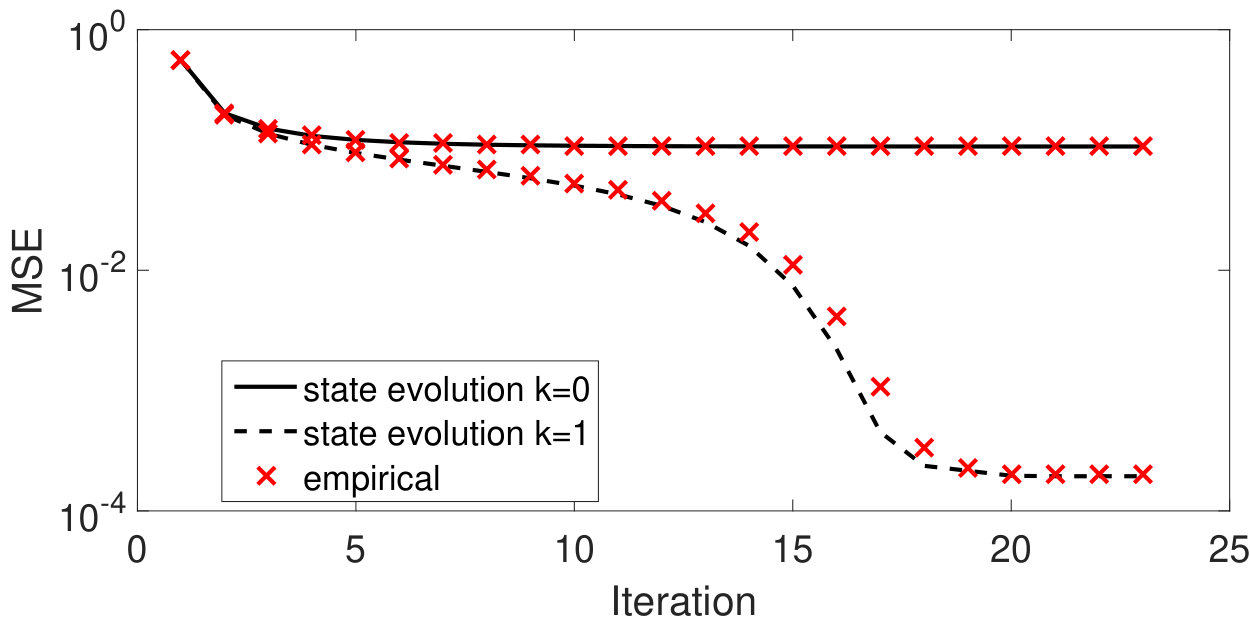 Figure 1
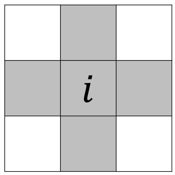 Figure 2
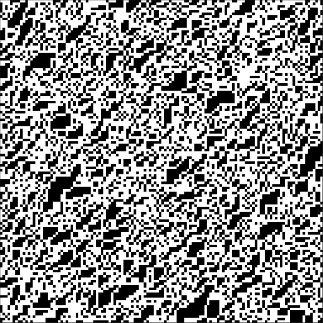 Figure 3
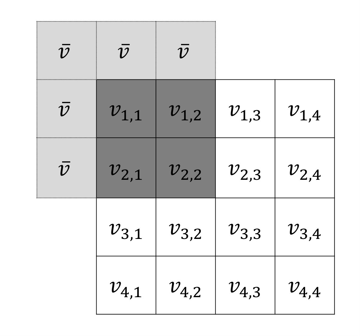 Figure 4
 Figure 5
 Figure 6
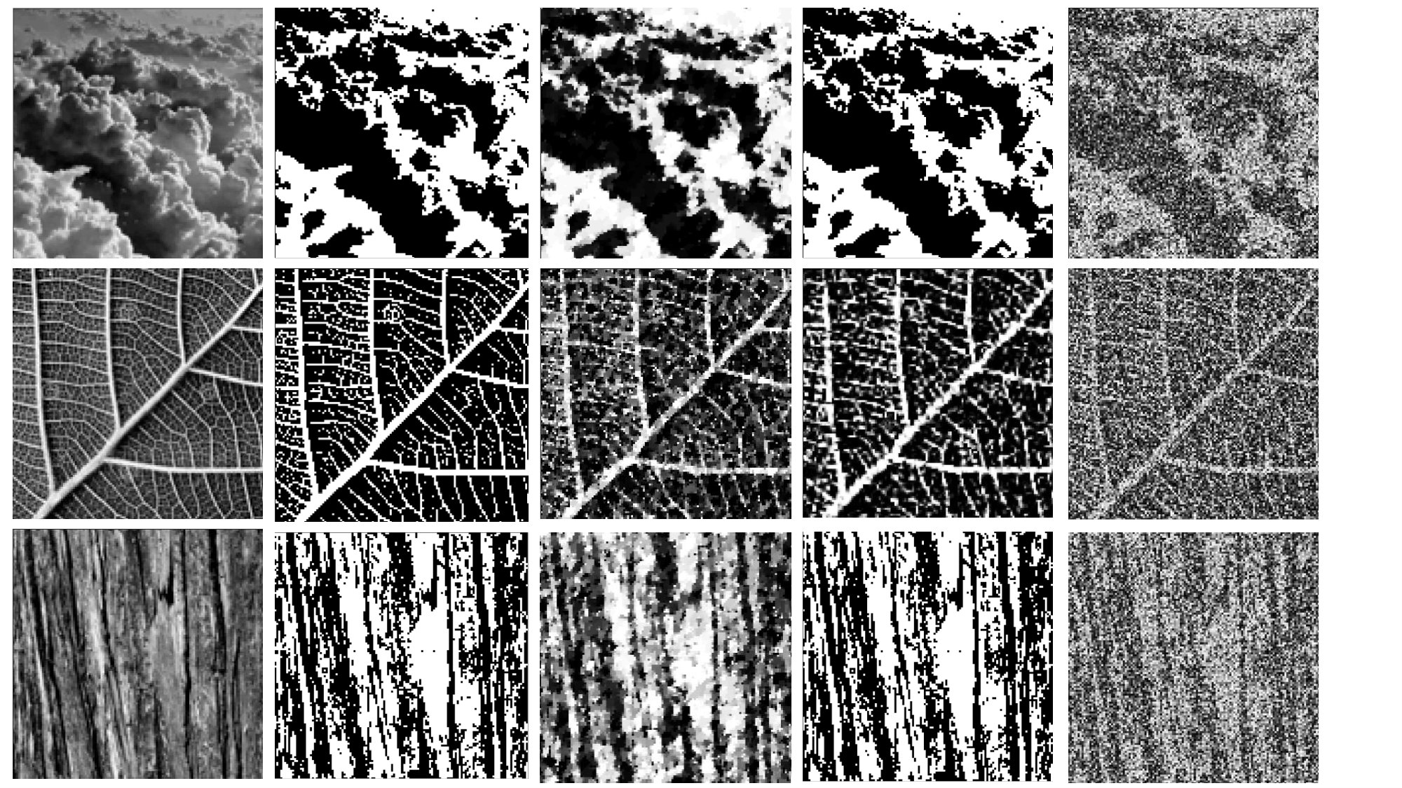 Figure 7
Peer Reviews
No public reviews on file for this paper yet. If you reviewed it on a platform where reviews are public (OpenReview, ICLR, NeurIPS, ICML), you can paste yours below so the community can read it here.
Videos
No videos yet. Explain this paper in a talk, walkthrough, or lecture? Add one.
Taxonomy
TopicsSparse and Compressive Sensing Techniques · Distributed Sensor Networks and Detection Algorithms · Blind Source Separation Techniques
Analysis of Approximate Message Passing
with Non-Separable Denoisers and
Markov Random Field Priors
Yanting Ma, Cynthia Rush, and Dror Baron Y. Ma is with Mitsubishi Electric Research Laboratories (MERL), Cambridge, MA 02138, USA (e-mail: [email protected]).C. Rush is with the Department of Statistics, Columbia University, New York, NY 10027, USA (e-mail: [email protected]).D. Baron is with the Department of Electrical and Computer Engineering, North Carolina State University, Raleigh, NC 27695, USA (e-mail: [email protected]).This work was supported by the National Science Foundation (NSF) under grants CCF-1217749 and ECCS-1611112.Portions of the work appeared at the IEEE International Symposium on Information Theory (ISIT), Aachen, Germany, June 2017 [1].The work was completed while Y. Ma was with North Carolina State University.
Abstract
Approximate message passing (AMP) is a class of low-complexity, scalable algorithms for solving high-dimensional linear regression tasks where one wishes to recover an unknown signal from noisy, linear measurements. AMP is an iterative algorithm that performs estimation by updating an estimate of the unknown signal at each iteration and the performance of AMP (quantified, for example, by the mean squared error of its estimates) depends on the choice of a “denoiser” function that is used to produce these signal estimates at each iteration.
An attractive feature of AMP is that its performance can be tracked by a scalar recursion referred to as state evolution. Previous theoretical analysis of the accuracy of the state evolution predictions has been limited to the use of only separable denoisers or block-separable denoisers, a class of denoisers that underperform when sophisticated dependencies exist between signal entries. Since signals with entrywise dependencies are common in image/video-processing applications, in this work we study the high-dimensional linear regression task when the dependence structure of the input signal is modeled by a Markov random field prior distribution. We provide a rigorous analysis of the performance of AMP, demonstrating the accuracy of the state evolution predictions, when a class of non-separable sliding-window denoisers is applied. Moreover, we provide numerical examples where AMP with sliding-window denoisers can successfully capture local dependencies in images.
Index Terms:
approximate message passing, non-separable denoiser, Markov random field, finite sample analysis.
I Introduction
In this work, we study the problem of estimating an unknown signal from noisy, linear measurements as in the following model:
[TABLE]
where for some integer , is an index set with cardinality , is the output, is a known measurement matrix, is zero-mean noise with finite variance , and (script stands for “vectorization”) is an invertible operator that rearranges elements of an array into a vector, hence is a length- vector. We assume that the ratio of the dimensions of the measurement matrix is a constant value, , with .
Approximate message passing (AMP) [2, 3, 4, 5, 6] is a class of low-complexity, scalable algorithms studied to solve the high-dimensional regression task of (1). The performance of AMP depends on a sequence of functions used to generate a sequence of estimates from effective observations computed in every iteration of the algorithm. A nice property of AMP is that under some technical conditions these observations can be approximated as the input signal plus independent and identically distributed (i.i.d.) Gaussian noise. For this reason, the functions are referred to as “denoisers.”
Previous analysis of the performance of AMP only considers denoisers that act coordinate-wise when applied to a vector; such denoisers are referred to as separable. If the unknown signal has a prior distribution with i.i.d. entries, restricting consideration to only separable denoisers causes no loss in performance. However, in many real-world applications, the unknown signal contains dependencies between entries, and therefore a coordinate-wise independence structure does not approximate the prior for well. Instead of using a separable denoiser, non-separable denoisers can improve reconstruction quality for signals with such dependencies among entries. For example, when the signals are images [7, 8] or sound clips [9], non-separable denoisers outperform reconstruction techniques based on over-simplified i.i.d. models. In such cases, a more appropriate model might be a finite memory model, well-approximated with a Markov random field (MRF) prior. In this paper, we extend the previous performance guarantees for AMP to a class of non-separable sliding-window denoisers when the unknown signal is a realization of an MRF. Sliding-window schemes have been studied for denoising signals with dependencies among entries by, for example, Sivaramakrishnan and Weissman [10, 11]. MRFs are appropriate models for many types of images, especially texture images, which have an inherently random component [12, 13].
When the measurement matrix has i.i.d. Gaussian entries and the empirical distribution function111For a vector , the empirical distribution function is defined as , where denotes the indicator function. The empirical distribution function is said to converge to some distribution function if for all such that is continuous, we have . of the unknown signal converges to some distribution function on , Bayati and Montanari [4] proved that at each iteration the performance of AMP can be accurately predicted by a simple, scalar iteration referred to as state evolution in the large system limit ( such that is a constant). For example, if is the estimate produced by AMP at iteration , the result by Bayati and Montanari [4] implies that the normalized squared error, , and other performance measures converge to deterministic values predicted by state evolution, which is a deterministic recursion calculated using the prior distribution of .222Throughout the paper, denotes the sum of squares of all the entries in , where could be, for example, in , , or . Rush and Venkataramanan [14] provided a concentration version of the asymptotic result when the prior distribution of is i.i.d. sub-Gaussian. The result in Rush and Venkataramanan [14] implies that the probability of -deviation between various performance measures and their limiting constant values decay exponentially in .
Extensions of AMP performance guarantees beyond separable denoisers have been considered in special cases [15, 16] for certain classes of block-separable denoisers that allow dependencies within blocks of the signal with independence across blocks. A preliminary version [1] of this work has analyzed the performance of AMP with sliding-window denoisers applied to the setting where the unknown signal has a Markov chain prior. In this paper, we generalize the previous result with the applications of compressive imaging [7, 8] and compressive hyperspectral imaging [17] in mind. We consider 2D/3D MRF priors for the input signal , and provide performance guarantees for AMP with 2D/3D sliding-window denoisers under some technical conditions.
While we were concluding this manuscript, we became aware of recent work of Berthier et al. [18]. The authors prove that the loss of the estimates generated by AMP (for a class of loss functions) with general non-separable denoisers converges to the state evolution predictions asymptotically. Our work differs from [18] in the following three aspects: (i) our work provides finite sample analysis, whereas the result in [18] is asymptotic; (ii) we adjust the state evolution sequence for the specific class of non-separable sliding-window denoisers to account for the “edge” issue that occurs in the finite sample regime (this point will become clear in later sections); (iii) we consider the setting where the unknown signal is a realization of an MRF and the expectation in the definition of the state evolution sequence is with respect to (w.r.t.) the signal , the matrix , and the noise , whereas in [18], the signal is deterministic and unknown, hence the expectation is only w.r.t. the matrix and the noise .
I-A Sliding-Window Denoisers and AMP Algorithm
Notation: Before introducing the algorithm, we provide some notation that is used to define the sliding window in the sliding-window denoiser. Without loss of generality, we let the index set , on which the input signal in (1) is defined, be
[TABLE]
where for an integer , the notation represents the set of integers , hence, . Similarly, let be a -dimensional cube in with length in each dimension, namely,
[TABLE]
where . We call the half-window size.
AMP with sliding-window denoisers: The AMP algorithm for estimating from and in (1) generates a sequence of estimates , where , is the iteration index, and the initialization is an all-zero array with the same dimension as the input signal . For , the algorithm proceeds as follows:
[TABLE]
where the function is a sequence of denoisers, is the partial derivative w.r.t. the center coordinate of the argument, is the transpose of , and for each is the -dimensional cube translated to be centered at location . The translated -dimensional cubes are referred to as “sliding windows,” which will be used to subset elements of a -dimensional array. The effective observation at iteration is , which can be approximated as the true signal plus i.i.d. Gaussian noise (in a sense that will be made clear in the statement of our main result, Theorem 1). Note that the sliding-windows and the sliding-window denoiser are defined on multidimensional signals, hence we use the inverse of the vectorization operator, , to rearrange elements of vectors into arrays before applying the sliding-window denoiser . It should also be noted that the denoiser may only process part of the signal elements in . For example, in the 2D case, if is defined as a window, then may only process the center and the four adjacent pixel values in the window (see Figure 1) and ignore the four corners. To simplify notation, we will write throughout the paper, and interpret this notation to mean that any processing of neighboring signal values is allowed, including the possibility of ignoring some of their values.
Edge cases: Notice that when the center coordinate is near the edge of , some of the elements in may fall outside , meaning that where is the complement of w.r.t. . In the definition of the AMP algorithm with sliding-window denoisers and the subsequent analysis, these “edge cases” must be handled carefully. The following definitions provide a framework for the special treatment of the edge cases.
Based on whether has elements outside , we partition the index set into two sets and defined as:
[TABLE]
That is, for , all elements in lie inside , whereas for , some of the elements in fall outside . The size of each set will depend on the half-window size and the dimension .
For any , let be a subset of the elements of with indices in and for any , let be the index of so that returns a single element of . Notice that for , all entries of are well-defined. However, for , the subset has undefined entries, namely, for all such that , the entry is undefined. We now define the value of those “missing” entries to be the average of the entries of having indices in . Formally, for all such that , define
[TABLE]
It may improve signal recovery quality to use other schemes for “missing” entries, like interpolation. We leave the study of these improved schemes for future work, but the effect of improved processing around edges should become minor as increases. Notice that for all are now defined using only the entries in the original . It will be useful to emphasize this point in the proof of our main result, so we define a set of functions with as
[TABLE]
where follows our definition above. That is, is identity for , whereas for , extends a smaller array to a larger one with the extended entries defined by (7).
Examples for defining “missing” entries: To illustrate the notations defined above, we present an example for the case (hence is a vector). As defined above in (2) and (3), we have , , and for each . Moreover, and as defined in (6). Therefore, for ,
[TABLE]
For , the vector is still length-, and we set the values of the non-positive indices, i.e., , or indices above , i.e., , to be the average of values in the vector with indices in . For example, let and giving so that for we have . Following (7), define
[TABLE]
and so . An example for the case (hence is a matrix), is shown in Figure 2.
I-B Contributions and Outline
Our main result proves concentration for (order-2) pseudo-Lipschitz (PL(2)) loss functions333A function is (order-2) pseudo-Lipschitz if there exists a constant such that for all , . acting on the AMP estimate given in (5) at any iteration of the algorithm to constant values predicted by the state evolution equations that will be introduced in the following. This work covers the case where the unknown signal has an MRF prior on . For example, when , can be thought of as an image, whereas when , can be thought of as a hyperspectral image cube. Moreover we use numerical examples to demonstrate the effectiveness of AMP with sliding-window denoisers when used to reconstruct images from noisy linear measurements.
The rest of the paper is organized as follows. Section II provides model assumptions, state evolution formulas, the main performance guarantee, and numerical examples illustrating the effectiveness of the algorithm for compressive image reconstruction. Our main performance guarantee (Theorem 1) is a concentration result for PL loss functions acting on the AMP outputs from (4)-(5) to the state evolution predictions. Section III provides the proof of Theorem 1. The proof is based on a technical lemma, Lemma 4, and the proof of Lemma 4 is provided in Section IV.
II Main Results
II-A Definitions and Assumptions
First we include some definitions relating to MRFs that will be used to state our assumptions on the unknown signal . These definitions can be found in standard textbooks such as [19]; we include them here for convenience.
Definitions: Let be a probability space. A random field is a collection of random variables defined on having spatial dependencies, where for some measurable state space and is a non-empty, finite subset of the infinite lattice . Note that , hence . One can consider as a collection of spatial locations. Denote the -order neighborhood of location by , that is, is a collection of location indices at a distance less than or equal to from but not including . Formally,
[TABLE]
Following these definitions, is said to be a -order MRF if, for all and for all measurable subsets , we have
[TABLE]
and for all we have . The positivity condition ensures that the joint distribution of an MRF is a Gibbs distribution by the Hammersley-Clifford theorem [20].
Let denote the distribution measure of , namely for all , we have , and let be the distribution measure of for . For any , define the set . Then the random field is said to be stationary if for all such that , it is true that .
Next we introduce the Dobrushin uniqueness condition, under which the random field admits a unique stationary distribution. Define the Dobrushin interdependence matrix for the measure of the random field to be
[TABLE]
In the above, the index set and the total variation distance between two probability measures and on is defined as
[TABLE]
Note that if is countable, then
[TABLE]
The measure is said to satisfy the Dobrushin uniqueness condition if
[TABLE]
The Dobrushin contraction coefficient, , is a quantity that estimates the magnitude of change of the single site conditional expectations, as they appear in (9), when the field values at the other sites vary. Similarly, we define the transposed Dobrushin contraction condition as
[TABLE]
Assumptions: We can now state our assumptions on the signal , the matrix , and the noise in the linear system (1), as well as the denoiser function used in the algorithm (4) and (5).
Signal: Let be a bounded state space (countable or uncountable). Let be a stationary MRF with Gibbs distribution measure on , where is a finite and nonempty rectangular lattice. We assume that satisfies the Dobrushin uniqueness condition and the transposed Dobrushin uniqueness condition. These two conditions together are needed for the results in Lemma C.1 and Lemma C.2, which demonstrate concentration of sums of pseudo-Lipschitz functions when the input to the functions are MRFs with distribution measure . Roughly, the conditions ensure that the dependencies between the terms in the sums are sufficiently weak for the desired concentration to hold. The class of finite state space stationary MRFs, which is widely used for image analysis [21], is one example that satisfies our assumption.
Denoiser functions: The denoiser functions used in (5) are assumed to be Lipschitz444A function is Lipschitz if there exists a constant such that for all , . for each and are, therefore, also weakly differentiable with bounded (weak) partial derivatives. We further assume that the partial derivative w.r.t. the center coordinate of , which is denoted by , is itself differentiable with bounded partial derivatives. Note that this implies is Lipschitz. (It is possible to weaken this condition to allow to have a finite number of discontinuities, if needed, as in [14].)
Matrix: The entries of the matrix are i.i.d. .
Noise: The entries of the measurement noise vector are i.i.d. according to some sub-Gaussian distribution with mean 0 and finite variance . The sub-Gaussian assumption implies [22] that for all and for some constants ,
[TABLE]
II-B Performance Guarantee
As noted in Section I, the behavior of the AMP algorithm is predicted by a deterministic scalar recursion referred to as state evolution, which we now introduce. More specifically, the state evolution sequences and defined below in (11) will be used in Theorem 1 to characterize the estimation error of the estimates produced by AMP. Let the joint distribution define the (stationary) prior distribution for the unknown signal in (1). Following our assumption of stationarity, for all and for all with defined in (6), where and denote the one-dimensional marginal and -dimensional marginal of , respectively. Define , and . Iteratively define the state evolution sequences and as follows:
[TABLE]
where is the sliding-window denoiser and has i.i.d. standard normal entries, independent of , which implies that is independent of and for all . Let and define with entries that are i.i.d. . We notice that for all , we have and . Therefore, for all , the expectations in (11) satisfy , where is the center coordinate of . For with defined in (6), it is not necessarily true that since, by definition (7), some entries of are defined as the average of other entries.
The explicit expression for the definition of in (11) is different when considering for different values, as the size of the set depends on the dimension. In the following, we provide explicit expressions for for the cases , but in the proof we will use the general expression given in (11) for brevity. We emphasize that the definition of the state evolution sequence in (11) only uses the marginal distribution (or ) instead of the joint distribution (or ), as demonstrated in the two examples below in (12) and (13).
Examples for explicit expressions for : Let be the center coordinate of and the window translated with center . Recall that is the -dimensional cube with length in each of the dimensions. Then we have and when we consider shifts for we, analogous to the definition in (7), define “missing” entries to be replaced by the average of the existing entries. (Note that since is exactly of size , thus for any , there will be “missing” entries.) For example, when ,
[TABLE]
where . Generalizing, we have with
[TABLE]
The same idea can be extended when .
For the case , we note that and , hence and . Therefore, we have
[TABLE]
where . In the above the first term corresponds to the middle indices, while the second term sums over terms corresponding to all the possible edge cases.
For the case , we note that , hence . Here we note . Therefore,
[TABLE]
where we notice that there are terms in the second summand, terms in the third and fourth summands, and . Again, in the above the first term sums over all the middle indices. In this case, the second term corresponds to the corner edge cases, while the third and fourth terms correspond to the edge cases in one dimension only. We note that is a function of , but do not explicitly represent this relationship to simplify the notation. Moreover, for fixed , the terms , , and vanish as goes to infinity. Therefore, we have .
Similar to [14], our performance guarantee, Theorem 1, is a concentration inequality for PL(2) loss functions at any fixed iteration , where is the first iteration when either or defined in (36) is smaller than a predefined quantity . The precise definition of and is deferred to Section III-B. For now, we can understand (respectively, ) as a number that quantifies (in a probabilistic sense) how close an estimate (respectively, a residual ) is to the subspace spanned by the previous estimates (respectively, the previous residuals ). In the special case where are Bayes-optimal conditional expectation denoisers, it can be shown that small implies that the difference between and is small [14].
Theorem 1**.**
Under the assumptions stated in Section II-A, and for fixed half window-size , then for any (order-) pseudo-Lipschitz function , , and ,
[TABLE]
where , has i.i.d. standard normal entries and is independent of , and the deterministic quantity is defined in (11). The constants do not depend on or , but do depend on and . Their values are not explicitly specified.
Proof.
See Section III. ∎
Remarks:
(1) The probability in (14) is w.r.t. the product measure on the space of the matrix , signal , and noise .
(2) By choosing the following PL(2) loss function, , Theorem 1 gives the following concentration result for the mean squared error of the estimates. For all ,
[TABLE]
with defined in (11).
II-C Numerical Examples
Before moving to the proof of Theorem 1, we first demonstrate the effectiveness of the AMP algorithm with sliding-window denoisers when used to reconstruct an image from its linear measurements acquired according to (1). We verify that state evolution accurately tracks the normalized estimation error of AMP, as is guaranteed by Theorem 1. While we use squared error as the error metric in our examples, which corresponds to the case where the PL(2) loss function in Theorem 1 is defined as , we remind the reader that Theorem 1 also supports other PL(2) loss functions. Moreover, we apply AMP with sliding-window denoisers to reconstruct texture images, which are known to be well-modeled by MRFs in many cases [12, 13].
II-C1 Verification of state evolution
We consider a class of stationary MRFs on whose neighborhood is defined as the eight-nearest neighbors, meaning this is a -order MRF per the definition in Section II-A. The joint distribution of such an MRF on any finite rectangular lattice in has the following expression [23]:
[TABLE]
where we follow the notation in [23] for the generic measure defined as
[TABLE]
and the conditional distribution of the element in the box given the element(s) not in the box:
[TABLE]
The generic measure needs to satisfy some consistency conditions to ensure the Markovian property and stationarity of the MRF on a finite grid; details can be found in [23]. For convenience, in simulations we use a Binary MRF as defined in [23, Definition 7], for which the generic measure is conveniently parameterized by four parameters, namely,
[TABLE]
In the simulations, we set . Using (9) and (10), it can be checked that the distribution measure of this MRF satisfies the Dobrushin uniqueness condition.
As mentioned previously, an attractive property of AMP, which is formally stated in Theorem 1, is the following: for large and and for , the observation vector used as an input to the estimation function in (5) is approximately distributed as , where , has i.i.d. standard normal entries, independent of , and is defined in (11). With this property in mind, a natural choice of denoiser functions are those that calculate the conditional expectation of the signal given the value of the input argument, which we refer to as Bayesian sliding-window denoisers. Let and , then for each we define
[TABLE]
where denotes the center coordinate of , denotes all coordinates in except the center, since coordinates of are i.i.d. normal, and is computed according to (15) with by using (16) and the property of Binary MRF given in [23, Definition 7]. Figure 4 shows that the MSE achieved by AMP with the non-separable sliding-window denoiser defined above is tracked by state evolution at every iteration.
Notice that when , the denoisers are separable and since the empirical distribution of converges to the stationary probability distribution on , the state evolution analysis for AMP with separable denoisers () was justified by Bayati and Montanari [4]. However, it can be seen in Figures 3 and 4 that the MSE achieved by the separable denoiser () is significantly higher (worse) than that achieved by the non-separable denoisers ().
II-C2 Texture Image Reconstruction
We now use the Bayesian sliding-window denoiser defined in (17) to reconstruct binary texture images shown in Figure 5. The MRF prior is the same type as described in Section II-C1, namely the Binary MRF, but we set the parameters . Note that while it is possible to learn an MRF model for each of the images using well-established MRF learning algorithms, we do not include this procedure in our simulations since the study of texture image modeling is beyond the scope of this paper. Moreover, the reconstruction results obtained using the simple MRF defined above are sufficiently satisfactory, despite the fact that the prior may be inaccurate. In Figure 5, we begin with natural images of a cloud, a leaf, and wood ( column) and then use thresholding to generate binary test images ( column). In addition to presenting the reconstructed images obtained by the Bayesian sliding-window denoisers with ( column) and ( column), respectively, we also present those obtained by AMP with a total variation denoiser [24] as a baseline approach ( column).
III Proof of Theorem 1
The proof of Theorem 1 follows the work of Rush and Venkataramanan [14], with modifications for the dependent structure of the unknown vector in (1). For this reason, we use much of the same notation. We prove Theorem 1 using a technical lemma, Lemma 4, which corresponds to [14, Lemma 6]. Before stating the lemma, we cover some preliminary results and establish notation to be used in its proof.
III-A Proof Notation
As in the previous work by Bayati and Montanari [4], as well as the work by Rush and Venkataramanan [14], the technical lemma is proved for a more general recursion, with AMP being a specific example of the general recursion as shown below. The connection between AMP and the general recursion will be explained in (25) and (26).
Fix the half-window size , an integer. Let and be sequences of Lipschitz functions. Specifically, the arguments of are two variables in , for example, for , we write and call the first argument of . Given noise and unknown signal , define vectors and , as well as arrays (for which and are the vectorized versions) for recursively as follows. Starting with initial condition :
[TABLE]
with the scalars defined as
[TABLE]
where the derivative of is w.r.t. the first argument, and the derivative of is w.r.t. the center coordinate of the first argument. In the context of AMP, as made explicit in (25), the terms and measure the error in the observation and the estimate at time , respectively, (the error w.r.t. the true ). The term measures the residual at time and the term is the difference between the noise and residual at time .
Recall that the unknown vector is assumed to have a stationary MRF prior with joint distribution measure . Let and be an all-zero array. Define
[TABLE]
Further, for all let
[TABLE]
and assume that there exist constants such that
[TABLE]
Define the state evolution scalars and for the general recursion as follows,
[TABLE]
where random variables and are independent and random arrays and with i.i.d. entries are also independent. We assume that both and are strictly positive. The technical lemma will show that can be approximated as i.i.d. in functions of interest for the problem, namely when used as an input to PL functions, and can be approximated as i.i.d. in PL functions. Moreover, it will be shown that the probability of the deviations of the quantities and from and , respectively, decay exponentially in .
We note that the AMP algorithm introduced in (4) and (5) is a special case of the general recursion of (18) and (19). Indeed, define the following vectors recursively for , starting with and ,
[TABLE]
It can be verified that these vectors satisfy (18) and (19) using Lipschitz functions
[TABLE]
where and . Using the choice of given in (26) also yields the expressions for given in (11). In the remaining analysis, the general recursion given in (18) and (19) is used. Note that in AMP, and , hence, assumption (23) for AMP requires
[TABLE]
Under our assumptions for as stated in Section II-A, we see that (27) is satisfied using Lemma C.2 (Appendix C), since the function is pseudo-Lipschitz. Finally, note that if we assume and , then the condition of strict positivity of and defined in (24) is satisfied.
Let denote a matrix with columns . For , define matrices
[TABLE]
Moreover, , , , are defined to be the all-zero vector.
The values and are projections of and onto the column space of and , with and being the projections onto the orthogonal complements of and . Finally, define the vectors
[TABLE]
to be the coefficient vectors of the parallel projections, i.e.,
[TABLE]
The technical lemma, Lemma 4, shows that for large , the entries of the vectors and concentrate to constant values, which are defined in the following section.
III-B Concentrating Constants
Recall that is the unknown vector to be recovered and is the measurement noise. In this section we introduce the concentrating values for inner products of pairs of the vectors that are used in Lemma 4.
Let be a sequence of zero-mean jointly Gaussian random variables taking values in , and let be a sequence of zero-mean jointly Gaussian random arrays taking values in . The covariance of the two random sequences is defined recursively as follows. For , ,
[TABLE]
where
[TABLE]
Note that both terms of the above (32) are scalar values and we take , the initial condition. Moreover, and , as can be seen from (24), thus for all , we have . Therefore, has i.i.d. entries.
Next, we define matrices and vectors whose entries are and defined in (32): for ,
[TABLE]
Lemma 1 below shows that and are invertible. Therefore, we can define the concentrating values for and defined in (29) as
[TABLE]
as well as the values of and for :
[TABLE]
For , we let and . Finally, define the concentrating values for and defined in (19) as
[TABLE]
Lemma 1**.**
If and are bounded below by some positive constants for , then the matrices and defined in (33) are invertible for .
Proof.
The proof follows directly as that of [14, Lemma 1] and therefore is not restated here. To see that this is the case, note that the proof of [14, Lemma 1] relies only on the relationship between (resp. ) and (resp. ) as defined in [14, (4.19)], which is the same as (36), and not the actual values taken by these objects. Therefore, the proof for [14, Lemma 1] applies here.
∎
III-C Conditional Distribution Lemma
As mentioned previously, the proof of Theorem 1 relies on a technical lemma, Lemma 4, stated in Section III-D and proved in Section IV. Lemma 4 uses the conditional distribution of the vectors and given the matrices in (28) as well as . Two forms of the conditional distribution of will be provided in Lemmas 2 and 47, which correspond to [14, Lemma 4] and [14, Lemma 5], respectively. Lemma 47 explicitly shows that the conditional distribution of can be represented as the sum of a standard Gaussian vector and a deviation term, where the explicit expression of the deviation term is provided in Lemma 2. Then Lemma 4 shows that the deviation term is small, meaning that its normalized Euclidean norm concentrates on zero, and also provides concentration results for various inner products involving the other terms in recursion (18), namely .
The following notation is used. Considering two random variables and a sigma-algebra , we denote the relationship that the conditional distribution of given equals the distribution of by . We represent a identity matrix as , dropping the subscript when it is clear from the context. For a matrix with full column rank, is the orthogonal projection matrix onto the column space of , and . Define to be the sigma-algebra generated by the terms
[TABLE]
Lemma 2**.**
For the vector and defined in (18), the following conditional distribution holds for :
[TABLE]
where and are i.i.d. standard Gaussian random vectors that are independent of the corresponding conditioning sigma algebras. The term and for is defined in (35) and the term and in (36). The deviation terms are
[TABLE]
where is the identity matrix and for any matrix , is the orthogonal projection matrix onto the column space of . For , defining and ,
[TABLE]
Proof.
As in [14], the key theoretical insight in the proof is to study the distribution of conditioned on the sigma algebra where is either or , meaning one treats as random, and considers the output of the AMP algorithm up until the current iteration as fixed and given in the sigma-algebra. This is done by observing that conditioning on is equivalent to conditioning on the linear constraints
[TABLE]
(due to the relationships and for and given in (18)). Then it is straightforward to characterize the conditional distribution of a Gaussian matrix given linear constraints.
Since the sequences are all in the conditioning , this conditional distribution depends only on the relationship between the matrix and these fixed, given terms. This relationship, namely that specified via and , is the same here as in [14, Lemma 3], and so the proofs are identical. We therefore do not repeat the details. Although and are obtained from , which is separable in [14], but non-separable in our case, and are simply treated as fixed elements in the conditioning sigma-algebra and the fact that they are calculated via non-separable functions here does not change the proof.
Then one is able to specify the conditional distributions of and given and , respectively, using the conditional distribution of . Again since the relationship between and and is the same here as in [14], the details are identical to that provided in the proof of [14, Lemma 4] and are not repeated here. ∎
Note that Lemma 2 holds only when is invertible. The following lemma provides an alternative representation of the conditional distribution of for , and it explicitly shows that is distributed as an i.i.d. Gaussian random vector with entries plus a deviation term.
Lemma 3**.**
For , let be i.i.d. standard normal random vectors. Let . For , recursively define
[TABLE]
and a set of scalars with ,
[TABLE]
Let . Then for all we have
[TABLE]
where are jointly Gaussian with correlation structure defined in (31). Moreover,
[TABLE]
Proof.
First, we prove (46) by induction. For , . As the inductive hypothesis, assume . By (44), term is equal in distribution to , where is independent of for all . In what follows, we show
[TABLE]
Note that are all zero-mean Gaussian, and therefore so is the sum. We now study the variance and covariance of by demonstrating the following two results:
- (i)
For all ,
[TABLE] 2. (ii)
For and all ,
[TABLE]
First consider (i). We note,
[TABLE]
In the above, step follows from the fact that is independent of , step from the covariance definition (31) and the i.i.d. standard normal nature of elements of , and step from
[TABLE]
Next, consider (ii). We see that
[TABLE]
In the above, step follows since is independent of and step from (31). Finally, notice that where the first equality holds since the sum equals the inner product of the row of with and the second equality by definition of in (35).
Next, we prove (47), also by induction. For , by (38) we have . Assume that holds for as the inductive hypothesis. Then,
[TABLE]
In the above, the first equality uses (38) and the second the inductive hypothesis. The last equality follows by noticing that for and using (45). ∎
III-D Main Concentration Lemma
Lemma 4**.**
We use the shorthand to denote the concentration inequality , where denote constants depending on the iteration index and the fixed half-window size , but not on or . The following statements hold for and .
- (a)
For defined in (41) and (43),
[TABLE] 2. (b)
For (order-2) pseudo-Lipschitz functions ,
[TABLE]
The random vectors are jointly Gaussian with zero mean entries, which are independent of the other entries in the same vector with covariance across iterations given by (31), and are independent of . 3. (c)
Recall that the operator rearranges the elements of an array into a vector,
[TABLE] 4. (d)
For all ,
[TABLE] 5. (e)
For all ,
[TABLE] 6. (f)
For all ,
[TABLE] 7. (g)
For and , when the inverses exist, for all and :
[TABLE]
where and are defined in (35), 8. (h)
With defined in (36),
[TABLE]
III-E Proof of Theorem 1
Proof.
Applying part (b) of Lemma 4 to a PL(2) function ,
[TABLE]
where the random field is independent of having i.i.d. standard normal entries. Now for let
[TABLE]
where is the PL(2) function in the statement of the theorem. The function in (62) is PL(2) since is PL(2) and is Lipschitz. We therefore obtain
[TABLE]
The proof is completed by noting from (5) and (25) that . ∎
IV Proof of Lemma 4
We make use of concentration results listed in Appendices A, B, and C, where Appendix C contains concentration results for dependent variables that were needed to provide the new results in this paper. Note that the lemmas that are stated in Appendices are labeled by capital letters with numbers (e.g., Lemma A.1), whereas the lemmas that are stated in the body are labeled by numbers (e.g., Lemma 1).
The proof of Lemma 4 proceeds by induction on . We label as the results (48), (49), (50), (52), (54), (56), (58), (60) and similarly as the results (51), (53), (55), (57), (59), (61). The proof consists of four steps: (1) proving that holds, (2) proving that holds, (3) assuming that and hold for all and , then proving that holds, and (4) assuming that and hold for all and , then proving that holds.
The proof of steps (1) and (3) – the steps – follow as in [14]. To see that this is the case, notice that in the proof for [14, Lemma 6], the results given by - involve the sequence of functions and the sequence of vectors . In our case, the definition of the (separable) functions in (18) is the same that in [14, (4.1)] and the conditional distribution of given in Lemma 2 has the same expression as that in [14, Lemma 6]. Therefore, the proof of - in [14] is directly applicable here.
Now consider . When , it only involves , which has the same assumption in our case and in [14]. When , the proof uses induction hypothesis -, , and . The statement of those hypotheses have the same form as in [14]. Although the concentration constants in those hypotheses have different definitions in this paper due to using non-separable denoisers, it does not change the proof for , since the actual values of the concentration constants are not involved in the proof. Therefore, we do not repeat the proof of steps (1) and (3) here. In what follows, we only show steps (2) and (4).
For each step, in parts – of the proof, we use and to label universal constants, meaning that they do not depend on or , but may depend on and , in the concentration upper bounds.
IV-A Step 2: Showing that holds
Throughout the proof we will make use of a function that selects the center coordinate of its argument. For example, for ,
[TABLE]
We will only use in cases where such a “center point” is well-defined. Notice that is Lipschitz, since for all , where (respectively, ) is the center coordinate of (respectively, ). Moreover, if a function is defined as with arbitrary but fixed , then is Lipschitz, because . We are now ready to prove .
(a) The definition of is given in (41). First notice that by Lemma B.1, we have , where is a standard normal random variable on . Using this fact and (41), we have
[TABLE]
By applying the triangle inequality to the norm of the RHS of (64) and then applying Lemma A.1,
[TABLE]
Label the three terms on the right-hand side (RHS) of (65) as . We will show that each term is bounded by .
First consider .
[TABLE]
where step follows by Lemma A.3, Lemma A.7, and . To see that step in (66) holds, we notice that
[TABLE]
since if the two events on the left-hand side (LHS) of (67) hold, then using that ,
[TABLE]
Taking the complement on both sides of (67),
[TABLE]
Then step in (66) follows by the union bound.
Next consider .
[TABLE]
where step follows by similar justification as that for step in (66) and step follows by Lemma A.3, Lemma A.6, and .
Finally consider .
[TABLE]
where step follows by Lemma A.1 and step follows by Lemma A.2, , and the assumption on given in (23).
(b) Let and be the array versions of the vectors and , respectively. For , the left-hand side (LHS) of (49) can be bounded as
[TABLE]
Step follows from the conditional distribution of given in Lemma 2 (38) and since and . Step follows from Lemma A.1. Label the terms on the RHS of (68) as . We show that each of these terms is bounded above by
First, consider . Recall the definition of the functions for in (8), which extends an array in to an array in by defining the extended entries to be the average of the entries in the original array. For arbitrary but fixed , the function defined as is PL(2) by Lemma B.5. Then it follows from Lemma B.4 that the function defined as is PL(2), since is an array of i.i.d. standard norm random variables for all . Notice that by the definition of and . Therefore,
[TABLE]
where in step we use the definition of in (8) and step follows from Lemma C.2 by noticing from Lemma B.5 that the function is PL(2) for all .
Next, consider . We use iterated expectation to condition on the value of . Then an be expressed as an expectation as follows,
[TABLE]
Define the function as
[TABLE]
For any fixed , define a function as for each and note that it is PL(2) with PL constant upper-bounded by , where is the PL constant for and is such that for all , since by the pseudo-Lipschitz property of and the triangle inequality,
[TABLE]
Using as the PL constant for for all , then
[TABLE]
where the last inequality follows from Lemma C.4 by noticing that . Therefore, , since and don’t depend on (as it doesn’t show up in the pseudo-Lipschitz constant ).
Finally, consider , the third term on the RHS of (68).
[TABLE]
Step follows from the fact that is PL(2). Step uses by the triangle inequality, the Cauchy-Schwarz inequality, the fact that for , , where , and the following application of Lemma B.6:
[TABLE]
From (69), we have
[TABLE]
where we use Lemma A.7 and to obtain step .
(c) We first show concentration for . Let the function be defined as for any , where the operator is defined in (63). Then, using the fact that and for all , since has zero-valued mean and is independent of , we find
[TABLE]
Finally, note that is PL(2) since is Lipschitz by Lemma B.3, hence, we can apply to give the desired upper bound.
Next, we show concentration for . Recall, for all . The function defined as is PL(2) by Lemma B.3 since and are both Lipschitz. Notice that and for all since has zero-valued mean and is independent of . Therefore, using ,
[TABLE]
(d) The function defined as is PL(2) by Lemma B.3 since the operator defined in (63) is Lipschitz. Notice that and for all , which follows from the definition of in (31). Therefore, the result follows using , since
[TABLE]
(e) We prove concentration for , and the result for follows similarly. The function defined as is PL(2) by Lemma B.3, since and are Lipschitz. Notice that by (32) and . Hence, we have the desired upper bound using , since
[TABLE]
(f) The concentration of to follows from applied to the function , since is assumed to be Lipschitz, hence PL(2).
The only other result to prove is concentration for . The function defined as is PL(2) by Lemma B.3. Notice that . Moreover, let the function be defined as , where the function replaces the center coordinate of the second argument, which is in , with the first argument, which is in , a scalar. For example, . Then we have
[TABLE]
In the above, step follows from Stein’s Method, Lemma B.2, step follows from the definition of in (31) and the definition of , which is the partial derivative w.r.t. the center coordinate of the first arguments, and step follows from the definition of in (37) and the definition of in (32). Therefore, using , we have the desired upper bound, since
[TABLE]
(g) Note that and . By Lemma A.5 and (23),
[TABLE]
By the definitions in Section III-A, and Therefore,
[TABLE]
where follows from Lemma A.2 with \tilde{\epsilon}:=\min\Big{\{}\sqrt{\frac{\epsilon}{3}},\ \frac{\epsilon}{3\tilde{E}_{0,1}},\ \frac{\epsilon\sigma_{0}^{2}}{3}\Big{\}} and from (70) and .
(h) From the definitions in Section III-A, we have , and . We therefore have
[TABLE]
where the last inequality is obtained using for bounding the first term and by applying Lemma A.2 to the second term along with the concentration of in (23), , and Lemma A.4 (for concentration of the square).
IV-B Step 4: Showing that holds
The probability statements in the lemma and the other parts of are conditioned on the event that the matrices are invertible, but for the sake of brevity, we do not explicitly state the conditioning in the probabilities. The following lemma will be used to prove .
Lemma 5**.**
Let and . Then for ,
[TABLE]
Proof.
We can infer from the proof of [14, Lemma 6] that the proof of Lemma 5 involves induction hypotheses -, -, , and . Notice that the statements of these hypotheses have the same form as the corresponding statements in [14]. While the definition of the concentration constants in these hypotheses may be different for separable and non-separable denoisers, the proof uses the result that the quantities concentrate with desired rate rather than what the concentration constants are. Therefore, the proof for [14, Lemma 12], which is similar to the proof of [14, Lemma 6], is directly applicable here. ∎
We are ready to prove .
(a) Recall the definition of from Lemma 2 (43). Using Lemma B.1, where columns of the matrix form an orthogonal basis for the column space of , which are normalized such that , and is an independent random vector with i.i.d. entries. We can then write
[TABLE]
where and are defined in Lemma 5. By Lemma B.6,
[TABLE]
where we have used . Applying Lemma, with , A.1,
[TABLE]
We now show each of the terms in (71) has the desired upper bound. For ,
[TABLE]
where step follows from similar justification as that for step in (66) and step follows from induction hypotheses , , and Lemma A.3. Next, the second term in (71) is bounded as
[TABLE]
where step is obtained using induction hypothesis , Lemma A.7, and Lemma A.3. Since concentrates on by , the third term in (71) can be bounded as
[TABLE]
For the second term in (72), first bound the norm of as follows. Letting denote the column of , we have
[TABLE]
where step (d) follows from Lemma B.6 and step (e) uses for all . Therefore,
[TABLE]
Step is obtained from Lemma A.1 and step from Lemma A.6. Using (73), the RHS of (72) is bounded by . Finally, for , the last term in (71) can be bounded by
[TABLE]
where step follows from Lemma 5, the induction hypothesis , and Lemma A.3. Thus we have bounded each term of (71) as desired.
(b) For brevity, we use the notation and
[TABLE]
for . Hence and are arrays in with entries , . We note that by we mean for the -dimensional cube to be applied to each of the elements of and we define . Moreover, define , hence , for all . Then, using the conditional distribution of from Lemma 47 and Lemma A.1,
[TABLE]
Label the terms of (75) as and . We next show that both terms are bounded by .
First consider term . Let . Notice that
[TABLE]
In the above, follows from Cauchy-Schwartz and by collecting the terms in the sums. Hence,
[TABLE]
Denote the RHS of (76) by , then using Lemma A.1 and , we have
[TABLE]
Now, using the pseudo-Lipschitz property of , we have
[TABLE]
Above, step follows from Cauchy-Schwartz and step from an application of Lemma B.6:
[TABLE]
and along with (76). Step follows from . Notice that
[TABLE]
where the last step follows from Lemma 47. Define . Then
[TABLE]
where the last step follows from Lemma A.7 and (27). Therefore, using the bound in (78),
[TABLE]
where the last step follows from (77) and (79).
Next, consider term of (75).
[TABLE]
Label the two terms on the RHS as and . can be bounded in a similar way as in (68) and has the desired bound by Lemma C.2, since the function defined as
[TABLE]
is PL(2) by Lemmas B.4 and B.5.
(c) We first show the concentration of . Using the PL(2) function defined in , we have that and for all , since has zero-valued mean and is independent of . Therefore, gives the desired upper bound, since
[TABLE]
We now show the concentration of . Using the PL(2) function defined in , we have that and , since has zero-valued mean and is independent of for all . Therefore, using , we have the desired upper bound, since
[TABLE]
(d) Let a function be defined as . Since the operator defined in (63) is Lipschitz, is PL(2) by Lemma B.3. Note that and , where the last equality follows from the definition in (31). Therefore, the result follows from , since
[TABLE]
(e) We will show the concentration of ; the concentration of follows similarly. The function defined as is PL(2) by Lemma B.3 and . Moreover,
[TABLE]
by definition (32). Therefore, using , we have the desired result, since
[TABLE]
(f) The concentration of around follows applied to the function , since is assumed to be Lipschitz, hence PL(2). Next, we show concentration for . Let be defined as , which is PL(2) by Lemma B.3. Note, and
[TABLE]
where the last equality follows using Stein’s Method, Lemma B.2, as in . Therefore, gives the desired result, since
[TABLE]
(g) We can represent as follows.
[TABLE]
Then, using and , it follows by the block inversion formula that
[TABLE]
Using definitions (35) and (36), block inversion can be similarly used to invert :
[TABLE]
In what follows, we show concentration for each of the elements in (81) to the corresponding elements in (86).
First, concentrates to at rate by and Lemma A.5. Next, consider the element of . For , using Lemma A.2 and as discussed in the previous paragraph,
[TABLE]
Consider element of for .
[TABLE]
Step follows from Lemma A.1 and Lemma A.2 with Step follows from the inductive hypothesis , together with (87).
We now prove . Recall, where . Thus, , for . Then by the definition of , for ,
[TABLE]
Step (a) follows from Lemma A.1 and step (b) from Lemma A.2, with . Step (c) uses and what we have just demonstrated in the previous paragraphs.
(h) First, note that . Using the definition of in (36), we then have
[TABLE]
By , the first term on the LHS of (88) is bounded by . For the second term, using ,
[TABLE]
Hence
[TABLE]
Step (a) follows from the concentration of products, Lemma A.2, using \tilde{\epsilon}_{i}:=\min\Big{\{}\sqrt{\frac{\epsilon}{6(t+1)}},\frac{\epsilon}{6(t+1)\tilde{E}_{i,t+1}},\frac{\epsilon}{6(t+1)\hat{\gamma}^{t+1}_{i}}\Big{\}}, and step (b) using and .
Appendix A Concentration Lemmas
In the following, is assumed to be a generic constant, with additional conditions specified whenever needed. The proof of the Lemmas in this section can be found in [14].
Lemma A.1**.**
(Concentration of Sums.) If random variables satisfy for , then
[TABLE]
Lemma A.2** (Concentration of Products).**
For random variables and non-zero constants , if
[TABLE]
then the probability P\Big{(}|XY-c_{X}c_{Y}|\geq\epsilon\Big{)} is bounded by
[TABLE]
Lemma A.3**.**
(Concentration of Square Roots.) Let . If
[TABLE]
then
[TABLE]
Lemma A.4** (Concentration of Powers).**
Assume and . Then for any integer , if
[TABLE]
then
[TABLE]
Lemma A.5** (Concentration of Scalar Inverses).**
Assume and . If
[TABLE]
then
[TABLE]
Lemma A.6**.**
For a standard Gaussian random variable and , .
Lemma A.7**.**
(-concentration.) For , that are i.i.d. , and ,
[TABLE]
Lemma A.8**.**
[22]** Let be a centered sub-Gaussian random variable with variance factor , i.e., , . Then satisfies:
For all , , for all . 2. 2.
For every integer ,
Appendix B Other Useful Lemmas
In this section, when the results are standard, they are presented without proof.
Lemma B.1**.**
[14, Fact 7]** Let be a deterministic vector and let be a matrix with independent entries. Moreover, let be a -dimensional subspace of for . Let be an orthogonal basis of with for , and let denote the orthogonal projection operator onto . Then for , we have where is a random vector with i.i.d. entries.
Lemma B.2**.**
(Stein’s lemma.) For zero-mean jointly Gaussian random variables , and any function for which and both exist, we have .
Lemma B.3**.**
(Products of Lipschitz Functions are PL(2).) Let be Lipschitz continuous. Then the product function defined as is PL(2).
Lemma B.4**.**
Let be defined in (3). For each , let be a constant and let have i.i.d. standard normal entries. Suppose is PL(2) with PL constant , then the function defined as is PL(2).
Proof.
Take arbitrary ,
[TABLE]
In the above, step follows from Jensen’s inequality, step holds since is PL(2) and using the triangle inequality, and step follows from . ∎
Lemma B.5**.**
Let and be as defined in (2) and (3), and let be translated to be centered at for each . Let be a PL(2) function with constant and define as , where is defined in (8). Then is PL(2) for all .
Proof.
Let be an arbitrary but fixed index in . Let , , and , so that counts the number of “missing” entries in . For any , we have that
[TABLE]
where step follows from the pseudo-Lipschitz property of and Lemma B.6, step from our definition of in (8), and step from Lemma B.6. ∎
Lemma B.6**.**
For any scalars and positive integer , we have . Consequently, for any vectors , .
Appendix C Concentration with Dependencies
We first state a concentration result, existing in the literature, for functions acting on random fields that satisfy the Dobrushin uniqueness condition in Lemma C.1. Then we use Lemma C.1 to obtain Lemma C.2, which is needed to prove .
Lemma C.1**.**
[25*, Theorem 1]**
Suppose that the random field taking values in is distributed according to a Gibbs measure that obeys the Dobrushin uniqueness condition with Dobrishin constant , and the transposed Dobrishin uniqueness condition with constant . Suppose that is a real function on with for all real . Then we have for all ,*
[TABLE]
Here is the variation vector of , where denotes the variation of at the site . Its -norm is defined as . If this norm is infinite, then the statement is empty (and thus correct).
Lemma C.2**.**
Let and be defined in (2) and (3), respectively, and let be a stationary Markov random field with a unique Gibbs distribution measure on . Assume that satisfies the Dobrushin uniqueness condition and the transposed Dobrushin uniqueness condition with constants and , respectively. Suppose that the state space is bounded, meaning that there exists an such that , for all . Let , where is being translated to be centered at location , be a PL(2) function with pseudo-Lipschitz constant , for all . Then for all there exist , such that
[TABLE]
Proof.
Let the function in Lemma C.1 be defined as . In order to apply Lemma C.1, we need to calculate . Let and , then we have that
[TABLE]
In the above, step uses the triangle inequality and the pseudo-Lipschitz property of . Step follows from the fact that for all and that for all . Therefore,
[TABLE]
Now applying Lemma C.1, we have
[TABLE]
∎
Lemma C.3 provides a technical result about pseudo-Lipschitz functions with sub-Gaussian inputs, which will be used to prove Lemma C.4.
Lemma C.3**.**
[1*, Lemma D.2]**
Let be a random vector whose entries have a sub-Gaussian marginal distribution with variance factor as in Lemma A.8. Let be an independent copy of . If is a PL(2) function with pseudo-Lipschitz constant , then the expectation satisfies the following for ,*
[TABLE]
Lemma C.4 provides a concentration inequality for sums of pseudo-Lipschitz functions acting on overlapping subsets of jointly Gaussian random variables.
Lemma C.4**.**
Let and be defined as in (2) and (3). For each , let have i.i.d. entries, and for all and , is independent of . Moreover, for each , let be jointly Gaussian with covariance matrix .
For each , define , where is translated to be centered at location . Let be a PL(2) function for all . Then for all , there exist such that
[TABLE]
Proof.
In the following, we prove the case for and the proof for other dimensions follows similarly. Without loss of generality, let and , hence . Further, assume without loss of generality that for all . In what follows, we demonstrate the upper-tail bound:
[TABLE]
and the lower-tail bound follows similarly. Together they provide the desired result.
Using the Cramér-Chernoff method, for all ,
[TABLE]
Let and be the pseudo-Lipschitz parameters associated with functions for and define . In the following, we will show that for ,
[TABLE]
where is any constant that satisfies . Then plugging (95) into (94), we can obtain the desired result in (93):
[TABLE]
Set , which is the choice that maximizes the term in the exponent in the above, i.e. it maximizes over . We can ensure that , falls within the region required in (95) by choosing large enough.
We now show (95). Define index sets
[TABLE]
for , and let denote the cardinality of . We notice that for any fixed , the ’s are i.i.d. for all . Also, we have , and , for , making the collection a partition of . Therefore,
[TABLE]
where are probabilities satisfying . Using the above,
[TABLE]
where step follows from Jensen’s inequality, step from the independence of ’s for , and step from Lemma C.3 with variance factor and restriction
[TABLE]
Let , where , ensuring . Then,
[TABLE]
whenever . In the above, step follows from:
[TABLE]
where step holds because and step holds because . Finally, we consider the effective region for as required in (97). Notice that
[TABLE]
Hence, if we require , then (97) is satisfied. ∎
The reference list from the paper itself. Each links out to its DOI / PubMed record.
- 1[1] Y. Ma, C. Rush, and D. Baron, “Analysis of approximate message passing with a class of non-separable denoisers,” Proc. IEEE Int. Symp. Inf. Theory , June 2017, full version: https://arxiv.org/abs/1705.03126 .
- 2[2] D. L. Donoho, A. Maleki, and A. Montanari, “Message passing algorithms for compressed sensing,” Proc. Nat. Academy Sci. , vol. 106, no. 45, pp. 18 914–18 919, Nov. 2009.
- 3[3] A. Montanari, “Graphical models concepts in compressed sensing,” in Compressed Sensing , Y. C. Eldar and G. Kutyniok, Eds. Cambridge University Press, 2012, pp. 394–438. [Online]. Available: http://dx.doi.org/10.1017/CBO 9780511794308.010 · doi ↗
- 4[4] M. Bayati and A. Montanari, “The dynamics of message passing on dense graphs, with applications to compressed sensing,” IEEE Trans. Inf. Theory , vol. 57, no. 2, pp. 764–785, Feb. 2011.
- 5[5] F. Krzakala, M. Mézard, F. Sausset, Y. Sun, and L. Zdeborová, “Probabilistic reconstruction in compressed sensing: Algorithms, phase diagrams, and threshold achieving matrices,” J. Stat. Mech. – Theory E. , vol. 2012, no. 08, p. P 08009, Aug. 2012.
- 6[6] S. Rangan, “Generalized approximate message passing for estimation with random linear mixing,” in Proc. IEEE Int. Symp. Inf. Theory (ISIT) , St. Petersburg, Russia, July 2011, pp. 2168–2172.
- 7[7] J. Tan, Y. Ma, and D. Baron, “Compressive imaging via approximate message passing with image denoising,” IEEE Trans. Signal Processing , vol. 63, no. 8, pp. 2085–2092, April 2015.
- 8[8] C. Metzler, A. Maleki, and R. G. Baraniuk, “From denoising to compressed sensing,” IEEE Trans. Inf. Theory , vol. 62, no. 9, pp. 5117 – 5114, Apr. 2016.