On Topologically Controlled Model Reduction for Discrete-Time Systems
Fredy Vides

TL;DR
This paper explores topologically controlled model reduction for discrete-time systems, linking data-driven approximation problems to constrained matrix representations within circulant matrices, and discusses algorithms and numerical results.
Contribution
It introduces a novel approach to model reduction by reducing problems to matrix representations in circulant algebra, with algorithms and numerical experiments.
Findings
Reduction of data-driven problems to circulant matrix representations
Development of algorithms for computing constrained matrix representations
Numerical implementations demonstrating the approach
Abstract
In this document the author proves that several problems in data-driven numerical approximation of dynamical systems in , can be reduced to the computation of a family of constrained matrix representations of elements of the group algebra in , factoring through the commutative algebra of circulant matrices in , for some integers . The solvability of the previously described matrix representation problems is studied. Some connections of the aforementioned results, with numerical analysis of dynamical systems, are outlined, a prorotypical algorithm for the computation of the matrix representations, and some numerical implementations of the algorithm, will be presented.
Click any figure to enlarge with its caption.
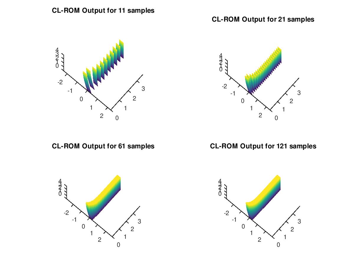 Figure 1
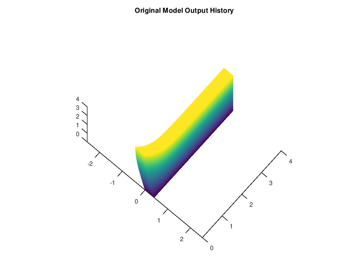 Figure 2
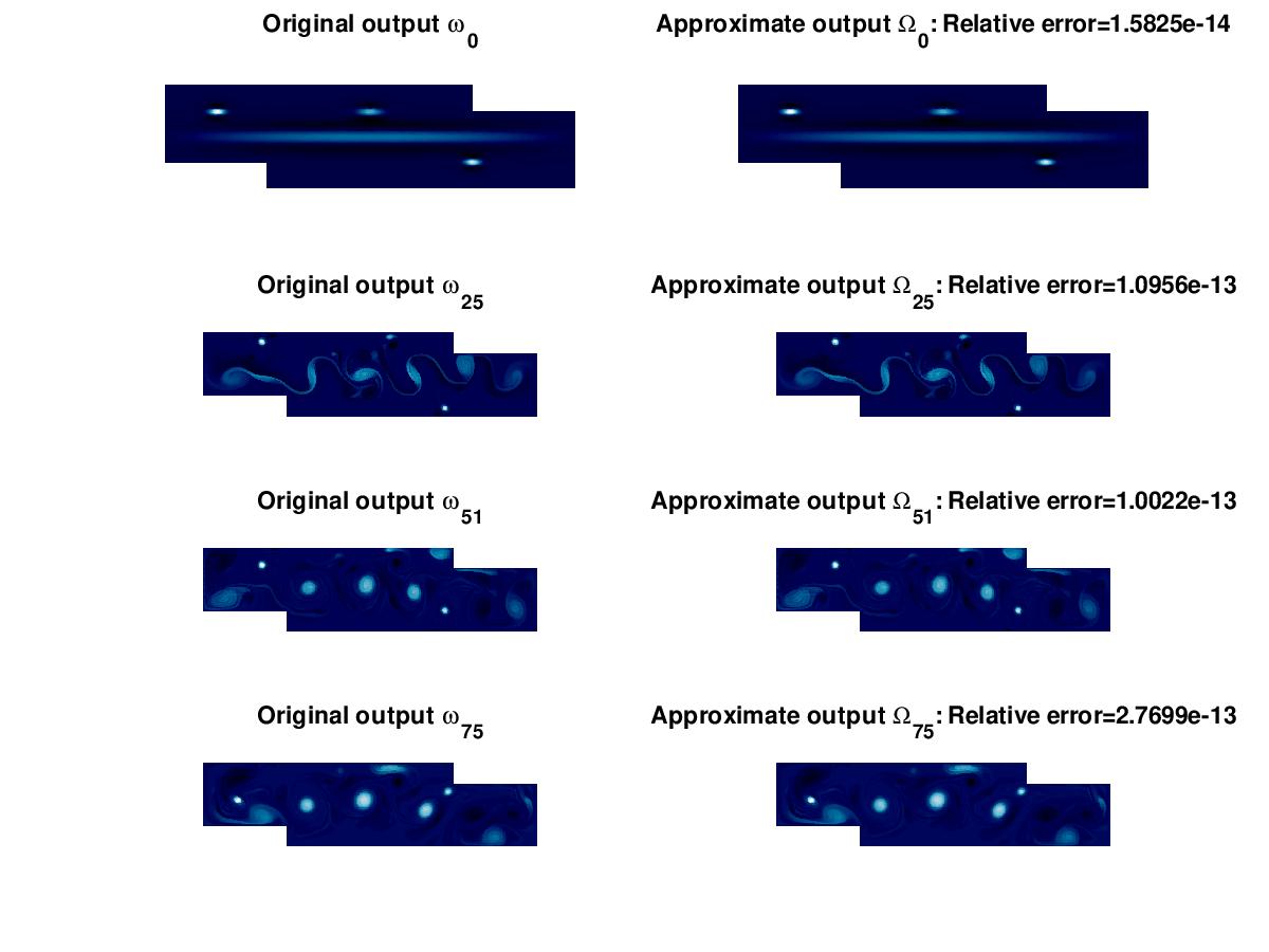 Figure 3
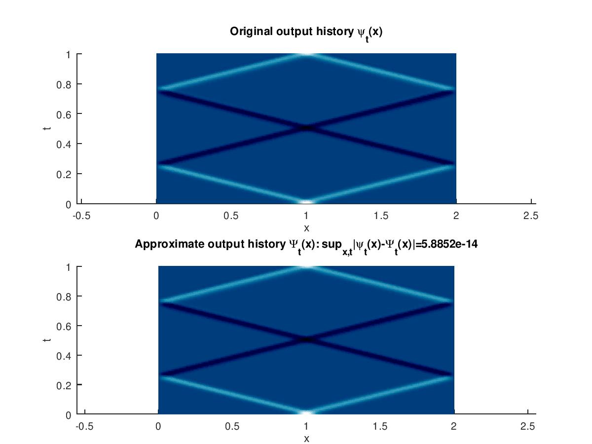 Figure 4
Peer Reviews
No public reviews on file for this paper yet. If you reviewed it on a platform where reviews are public (OpenReview, ICLR, NeurIPS, ICML), you can paste yours below so the community can read it here.
Videos
No videos yet. Explain this paper in a talk, walkthrough, or lecture? Add one.
Taxonomy
TopicsModel Reduction and Neural Networks · Numerical methods for differential equations · Control Systems and Identification
On Topologically Controlled Model Reduction for Discrete-Time Systems
Fredy Vides
Scientific Computing Innovation Center, Universidad Nacional Autónoma de Honduras, Tegucigalpa, Honduras
Abstract.
In this document the author proves that several problems in data-driven numerical approximation of dynamical systems in , can be reduced to the computation of a family of constrained matrix representations of elements of the group algebra in , factoring through the commutative algebra of circulant matrices in , for some integers .
The solvability of the previously described matrix representation problems is studied. Some connections of the aforementioned results, with numerical analysis of dynamical systems, are outlined, a prorotypical algorithm for the computation of the matrix representations, and some numerical implementations of the algorithm, will be presented.
Key words and phrases:
Group algebra, circulant matrices, discrete-time system, topological dynamics.
2010 Mathematics Subject Classification:
93B28, 47N70 (primary) and 93C57, 93B25 (secondary)
1. Introduction
In this document we will study discrete-time dynamical systems determined by the pair , with , and where is a family of continuous functions from to , such that and , for every pair of integers .
We will prove that several important problems in numerical analysis and data-driven discovery of discrete-time dynamical systems of the form in , can be reduced to the computation of a family of discrete-time transition matrices of rank at most with , for some matrix representation of the group algebra , together with two matrices of rank at most , that are related to some evolution history data , (approximately) generated by the dynamical , by the equations for .
We will also show that each variation of the problem corresponding to the computation of the aforementioned transition matrices, can be reduced to solving a constrained matrix representation problem of the group algebra in , factoring through the commutative algebra of circulant matrices in , for some integers .
The motivation for the theoretical and computational machinery presented in this document came from some questions raised by M. H. Freedman along the lines of [2], concerning to the implications in linear algebra and matrix computations of the so called Kirby Torus Trick, presented by R. Kirby in [3].
We study the solvability of the previously described matrix representation problems. Some connections of the aforementioned results, with numerical analysis of dynamical systems, are outlined, a prorotypical algorithm for the matrix representation computations, and some numerical implementations of the algorithm will be presented.
2. Preliminaries and Notation
Given two positive integers such that , we will write to denote the integer , such that for some integer . We will write to denote the set .
Given , we will write to denote the (additive) cyclic group .
Given any matrix , we will write to denote the entry of , and we will write to denote its conjugate transpose . We will identify elements in with elements in . As a consequence of this identification, given , will determine the Ecuclidean inner product in , while will determine a rank-one matrix in .
In this document we write and to denote the identity and zero matrices in and , respectively. We will write to denote the zero matrix in .
A set of elements is said to be an orthogonal -system if
[TABLE]
for .
From here on, we will write to denote the Kronecker delta defined by
[TABLE]
We say that the set of vectors is an orthonormal -system if the vectors satisfy (2.1) and in addition
[TABLE]
for .
We will write to denote the element in represented by the expression.
[TABLE]
Each can be interpreted as the -column of .
A matrix is said to be normal if , a matrix is said to be Hermitian if , and a hermitian matrix is said to be an orthogonal projection or just a projection, if .
A matrix is said to be unitary if . A matrix is said to be positive if there is a matrix such that , we also write to indicate that is positive. We will denote by and , the sets of unitaries and positive matrices in , respectively.
Given a matrix , we write to denote the linear map from to , defined by the operation for any .
We say that a matrix is invertible if there is one matrix such that . We will write to denote the set of invertible matrices in . Given a matrix , we will write to denote the spectrum of , that is the set .
From here on we write to denote the Euclidean norm in defined by the operation for any . In this document we will write to denote the spectral norm in defined by the opration , for any .
Definition 2.1**.**
A linear map is said to be a completely positive (CP) linear map if for every positive , and if it has a Choi’s representation of the form for some matrices .
We will write to denote the set of completely positve linear maps from to .
Given any and any determined by the formula , we will write to denote the matrix defined by the expression .
Given , we will write to denote the commutative algebra determined by the set , with respect to the usual addition and multiplication operations in . We have that in fact is an algebra since, for every integer , as a consequence of the Cayley-Hamilton Theorem, and that is commutative as a consequence of the identity , that holds for each and for each pair of integers .
We will write to denote the commutative algebra of Circulant matrices that is defined by the expression:
[TABLE]
where is the cyclic permutation matrix defined as follows.
[TABLE]
Given a matrix , we write to denote the commutant set of defined by the expression .
Given a finite group , we will write to denote the group algebra over .
For a finite group In this document we will focus on group algebra representations of determined by algebra homomorphisms of the form , such that is a group representation of in . We will say that an algebra representation is unitary if .
Given a discrete-time dynamical system , if there is an integer such that for each every , we say that is a discrete-time -periodic dynamical system.
Given a discrete-time dynamical system , a set of vectors will be called a -system of history vectors for , if they satisfy the relations for .
Given , we will say that a discrete-time dynamical system is -almost-periodic dynamical system, if there is a -periodic discrete-time dynamical system such that for each there is such that , and for each and every such that .
3. Topological Control Method (TCM)
3.1. Switched Closed Loop Reduced Order Models SCL-ROM
In this section we will stablish the notion of topological control considered for this study.
Given a discrete-time dynamical system with , and a -system of history vectors for , we say that , , is topologically controlled by a topological manifold or -controlled, if there is a matrix with , an algebra homomorphism , a family of polynomials , and two projections such that , for each . We will call the -tuple a topological control for .
Given and manifold , and a -controlled discrete-time dynamical system with , and a topological control , , for , we say that is a control of order , if there is an integer , together with maps , , such that and , for each , each , and some . In this case we say that is -controlled.
Given , a discrete-time dynamical system with , and a -system of history vectors for , we say that is -approximately topologically controlled by or -controlled, if there is a unitary representation , an algebra homomorphism , a family of functions , and two projections such that , for each and some , with .
For a given a discrete-time dynamical system with , and a -system of history vectors for , we approach the local controllability of by computing a switched closed loop control system in the sense of [1, §4.2,Example 4.2], determined by the decomposition.
[TABLE]
for some to be determined. Given , the discrete-time system (3.1) is called a -approximate swithed closed-loop reduced order model (SCL-ROM) of , if for each .
3.2. Some Connections with Dynamic Mode Decomposition
Given , an integer , and a discrete-time system in . Let us consider the evolution history determined by the difference equations.
[TABLE]
for some .
Given . The computation of a SCL-ROM local -approximant of , with respect to some sampled-data history of , is related to the computations of closed-loop matrix realizations and triples such that.
[TABLE]
The matrices in (3.3) are determined by the connecting operator for the sampled-data history , in the sense of [6, §2] and [4, §2.2], that satisfies the equations , , In particular we will consider , . The objective of topological control methods is to compute matrix realizations such that:
[TABLE]
for .
Given , an integer , a family of vectors in and matrices determined by the connecting operator for . For any triples that satisfy (3.3).
Let us consider the structured matrix equations in determined by:
[TABLE]
where and have the form.
[TABLE]
If we set.
[TABLE]
It can be seen that are -approximate solvent pairs for (3.4) in the sense that, , and for .
Given a positive integer , together with . In this first paper on the subject of topological control of discrete-time systems, we focus on the computation of transition mappings , avoiding an explicit computation of the connecting operator , instead we compute the family by solving some constrained representation problems for for a given integer , restricting our attention to almost -periodic discrete-time systems.
3.3. Main Objectives
We prove the solvability of the problem of finding a -approximate SCL-ROM described by (3.1) for a discrete-time system with a -system of history vectors , by computing matrix representations of such that the switching law of the family is controlled by some family subject to almost time-perdiodic constraints on . We will then design and implement a prototypical numerical algorithm that numerically solves the aforementioned problems.
3.4. Topologically Controlled Model Order Reduction
Let us consider an orthogonal -system with . From here on, we will write to denote the matrix in defined by the equation.
[TABLE]
where is the matrix in defined by the equation.
[TABLE]
Lemma 3.1**.**
Given an orthogonal -system with . The matrix defined by (3.6) is an orthogonal projection such that , . Moreover, is an orthogonal projection such that
Proof.
Given an orthogonal -system with . For each , let us set
[TABLE]
it is clear that each satisfies the relation,
[TABLE]
and we will also have that,
[TABLE]
By (3.8) and (3.9), we will have that , and this implies that each is projection, and by orthogonality ot the system , we have that
[TABLE]
This implies that the projections are mutually orthogonal projections, and it can be seen that . Moreover,
[TABLE]
We also have that.
[TABLE]
By (3.6) and by orthogonality of the system , we will have that for ,
[TABLE]
By (3.11) we will have that.
[TABLE]
As a consequence of (3.12) we will also have that.
[TABLE]
By (3.11) we will have that,
[TABLE]
and also that.
[TABLE]
This completes the proof. ∎
Lemma 3.2**.**
Given an orthogonal -system with . The matrices and defined by (3.5) and (3.6), respectively, satisfy the following conditions:
- •
, ,
- •
,
- •
,
- •
,
- •
.
Proof.
Since is defined by (3.5), by lemma 3.1, we will have that for :
[TABLE]
By lemma 3.1, and by (3.5) and (3.6), on one hand we will have that,
[TABLE]
on the other hand we will have that.
[TABLE]
By combining (3.21) and (3.22) we have that
[TABLE]
Since is an orthogonal projection, we will also have that.
[TABLE]
By (3.24) and (3.21), it can be seen that can be represented in the form.
[TABLE]
By lemma 3.1, we will have that,
[TABLE]
and also that.
[TABLE]
This completes the proof. ∎
Lemma 3.3**.**
Given an orthogonal -system with . The matrix defined by (3.5) satisfies the equation
[TABLE]
Moreover, is the minimal polynomial of .
Proof.
Given an orthogonal -system with . By (3.5), (3.6), and by iterating on lemma 3.2, we will have that.
[TABLE]
By orthogonality properties we have that the system is linearly independent. This fact combined with (3.29) implies that is the minimal polynomial of , since if for some , we would have that , which contradicts the linear independence of the system. ∎
Lemma 3.4**.**
Given an orthonormal -system with , we will have that the corresponding matrix is unitary.
Proof.
Given an orthonormal -system , since for each , by (3.5) we will have that the matrix satisfies the equation,
[TABLE]
and also that the matrix satisfies the equation.
[TABLE]
By lemma 3.2 we will have that,
[TABLE]
and also that.
[TABLE]
Since
[TABLE]
and
[TABLE]
by (3.30) and (3.31) we will have that.
[TABLE]
This implies that.
[TABLE]
This completes the proof. ∎
Lemma 3.5**.**
Given vectors such that , there is a orthonormal -system , two scalars , two projections , and a unitary in such that:
[TABLE]
for each .
Proof.
Let us consider the matrix defined by the expression.
[TABLE]
By the singular value decomposition theorem, we have that has a representation of the form.
[TABLE]
Where and are orthonormal -systems in and respectively, and with . Since , by the Gram-Schmidt orthonormalization theorem, we will have that there is an orthonormal -system . Since we will have that for each , . Let us set , for . We will have that and for each , since for every . Let us define the matrix by the expression.
[TABLE]
and
[TABLE]
Let us define the matrix by the expression.
[TABLE]
Since for each , by (3.39) and (3.40) and by orthogonality of the -system , we will have that . This implies that is an orthonormal -system. By lemma 3.4 we have that is a unitary matrix that satisfies the constraints , , and .
Let us set.
[TABLE]
Since we will have that and .
Since , we will have that , by (3.39) this implies that.
[TABLE]
We will first show that , in fact, since , and by orthogonality of , we will have that.
[TABLE]
We will also have that and .
Since , by (3.43) we have that . This completes the proof. ∎
Lemma 3.6**.**
Given an orthonormal -system with . There is determined by , such that the map from onto preserves products in , with determined by (3.6). Moreover, we will have that , and for any .
Proof.
Let us set.
[TABLE]
Since is an orthonormal -system, we will have that , by (3.6) we will have that.
[TABLE]
Since , by (3.45) we will have that,
[TABLE]
we will also have that for any .
[TABLE]
By (3.45) and (3.47) we will have that for any two .
[TABLE]
By (3.44) and by orthonormality of we will also have that for each .
[TABLE]
By (3.49) we have that , since and , we have that is surjective. This completes proof. ∎
Definition 3.1**.**
Given with , the matrix whose existence is proved in lemma 3.5 will be called a circular shift factor (CSF) for .
Lemma 3.7**.**
Given with , there is an algebra homomorphism from onto .
Proof.
By lemma 3.5 we have that there is an orthornormal -system together with a CSF . By lemma 3.5 we have that with determined by (3.6), this in turn implies that .
By lemma 3.6 there is such that is map from onto that preserves products in . Let us set . It is clear that .
By (3.47) and (3.49) we will have that.
[TABLE]
The identity (3.47) also implies that.
[TABLE]
Since preserves products in , for any two integers we will have that,
[TABLE]
and also that.
[TABLE]
By (3.52), (3.53) and (3.54), we will have that the map determines an algebra homomorphism from onto . ∎
Definition 3.2**.**
Given with , with corresponding CSF . The algebra homomorphism whose existence is warranteed by lemma 3.7, will be called a Circulant representation (CR) for
Theorem 3.1**.**
Given with , there is a projection together two maps and , such that the following diagram commutes,
[TABLE]
where is a CR of . Moreover, preserves products on and .
Proof.
By 3.5 there is an orthonormal -system together with projection such that for each . As a consequence of the argument implemented in the proof of lemma 3.7, we have that by lemma 3.6, there is a matrix such that and .
Let us set.
[TABLE]
It is clear that and . Given , we will have that.
[TABLE]
Since we will have that for any two .
[TABLE]
Since is a projection, for any , we will have that . This imples that .
By (3.2) we have that .
By (3.57) we will have that has a representation of the form.
[TABLE]
By (3.59) we will have that.
[TABLE]
This completes the proof. ∎
Given a discrete-time dynamical system with , and a -system of (history) vectors for , the matrix defined by the formula (3.41) for , will be called the orthonormal history factor (OHF) of .
Theorem 3.2**.**
Given , an integer , and a discrete-time -periodic dynamical system with , then is -controlled, for every and each such that .
Proof.
Given , and any vector history for , since , we can apply lemma 3.5 to compute an orthonormal -system , scalars , a CSF and two projections , that satisfy (3.36).
By theorem 3.1 we will have that there are a projection , and a product preserver such that and .
Since and are linear product preservers in and , respectively, we will have that for any .
[TABLE]
By theorem 3.1 we will have that,
[TABLE]
for each .
By (3.56) we have that , with defined by equation (3.6), by lemma 3.1 we will have that.
[TABLE]
Let , , this impies that . By lemma 3.5 and by (3.63), for each we will have that.
[TABLE]
By (3.62) and (3.64), we will have that is -controlled by . ∎
Theorem 3.3**.**
Given , an integer , and a discrete-time -periodic dynamical system with , then is -controlled, for every and each such that .
Proof.
Given , by theorem 3.2, we will have that is , , -controlled by some control .
We have that theorem 3.2 also implies that there is an algebra homomorphism such that , for each .
Since , we will have that and also that.
[TABLE]
By universality of there is a representation , determined by the assignment for .
Applying universality of to we have that,
[TABLE]
for each . This completes the proof. ∎
Theorem 3.4**.**
Given , every -almost-periodic dynamical system with is ()-controlled, whenever .
Proof.
Let . Since is -almost-periodic, we will have that there is a discrete-time -periodic dynamical system such that there is such that , and for each and every .
By theorem 3.2 we will have that is -controlled by some control , for some -system of history vectors , , with , this implies that for each .
[TABLE]
By (3.65) we have that is -controlled by , , , . This completes the proof. ∎
Theorem 3.5**.**
Given , every -almost-periodic dynamical system with is ()-controlled, whenever .
Proof.
Let . Since is -almost-periodic, we will have that there is a discrete-time -periodic dynamical system such that there is such that , and for each and every .
By theorem 3.3 we will have that is -controlled, this implies that for some -system of history vectors , , with , there is a unitary representation , an algebra homomorphism , a family of functions , and two projections such that for and for each .
[TABLE]
By (3.65) we have that is -controlled. This completes the proof. ∎
Given , from the definition in (3.1) of SCL-ROM approximants of a discrete-time system with , we have that by lemma 3.5 and theorem 3.4, every discrete-time system that is -controlled by some control , , , , has a SCL-ROM approximant of the form (3.1) with for , we say that such approximant is SCL-ROM is determined by the control , , , . We can think of the evolution laws for in SCL-ROM the decomposition (3.1), as an embedding of the original system in a manifold, where the evolution of the embedded system is controlled by a unitary matrix determined the CSF of some vector history for the original system.
4. Algorithm
The techniques and compuations used to prove the previous results, can be implemented to derive a prototypical algorithm described by the following block diagram.
[TABLE]
The proofs of lemma 3.5 and theorem 3.2 provide a computational procedure that is sketched in algorithm 1, and can be used to compute the elements in diagram (4.1), where each matrix has a reresentation , for some matrices , , to be determined by algorithm 1.
5. Experimental results
5.1. Materials and Methods
In order to solve the diagram (4.1), a prototypical GNU Octave code that implements some of the core computations on which the proofs of lemma 3.5 and theorem 3.2 are based, has been developed as part of this project, using GNU Octave 4.4.1 on a five node Ubuntu Linux Beowulf Cluster, at the Scientific Computing Innovation Center of UNAH-CU.
5.2. Numerical Experiments
We will consider three numerical experiments in this section. In §5.2.1 we will simulate 1D waves, in §5.2.2 we will simulate damped waves on planar material sections, and in §5.2.3 we will simulate vorticity transport.
In §5.2.1 the periodicity appears naturally, while in §5.2.2 and §5.2.3, we will think of the model as a movie, that is being streamed more than once. Each example will be used to illustrate the potential applications of topological control to system identification, and for extraction of (almost) periodic patterns from sampled-data discrete-time industrial systems and plants.
5.2.1. 1D Waves
As a first application, let us consider a wave equation under Dirichlet boundary conditions of the form:
[TABLE]
for some suitable data of .
The simulation is computed using second order finite difference method combined with second order Crank-Nicolson method. The computation is performed using the following commands.
[x,t,data_wave,Cx,Sx]=CL_ROM_WaveDS([0 1],10);
Running simulation:
Computing circular matrix representations in C[U[v1|vm]]:
The graphical output is shown in fig. 1.
5.2.2. Cantilever Elastic Plate
As a second application of algorithm 1, let us consider a computational mechanics problem consisting on the description of the deformation a damped aluminium Cantilever Lamé beam model under planar displacement hypotheses, whose deformation displacement vector is described by a Navier dynamical system of the form:
[TABLE]
where is the Navier operator defined by the expression,
[TABLE]
where are the Lamé’s coefficients for generic aluminium, and where is some system of equations that determines suitable boundary and initial conditions for Cantilever Lamé beam deflection. We will have that the input is determined by the expression for some smooth time dependent coefficient .
It is important to consider that the dimensions of the beam model have been normalized, and that relative deformation displacement scale is exaggerated for visualization purposes of the corresponding simulation.
In order to create the data corresponding to the beam deformation, we use an Octave m-file function that computes a second order finite difference approximation of the Navier dynamical system (5.2) for sample sizes , , and , as follows.
[Bx,By,data_x,data_y,Yx,Yy]=CL_ROM_BeamDS(1,50,40,-5e9,-10,1); [Bx,By,data_x,data_y,Yx,Yy]=CL_ROM_BeamDS(1,30,40,-5e9,-10,2); [Bx,By,data_x,data_y,Yx,Yy]=CL_ROM_BeamDS(1,10,40,-5e9,-10,3); [Bx,By,data_x,data_y,Yx,Yy]=CL_ROM_BeamDS(1,5,40,-5e9,-10,4);
Running simulation:
properties =
scalar structure containing the fields:
Emod = 73100000000
properties =
scalar structure containing the fields:
Emod =  73100000000
Nu =  0.33000
Lx =  4
Ly =  0.40000
T =  40
M =  600
N =  36
c2 =  0.35971
delta = -5000000000
m =  5
Elapsed time is 298.816 seconds.
Computing circular matrix representations in C[U[v1|vm]]:
Elapsed time is 3.51714 seconds.
Verifying circular mimetic constraints for C[U[v1|vm]]:
Verification passed... max{||Kx Rx Usx^k Tx Ux0-Oxk|| | 1<=k<=m} = 2.7082e-27 <= eps max{||Ky Ry Usy^k Ty Uy0-Oyk|| | 1<=k<=m} = 7.4542e-13 <= eps
For m = 121 For n = 13357 For eps = 7.4542e-13 Elapsed time is 20.7964 seconds.
This produces the original output history shown in Figure fig. 2.
The output histories of the corresponding SCL-ROM approximants are shown in Figure 3.
5.2.3. Planar vorticity transport
As a third application of local -control, let us consider the vorticity transport PDE system of the form.
[TABLE]
For Reynolds number and suitable boundary and initial conditions represented by the system of algebraic differential equaitons .
The simulation is computed using second order finite difference method combined with fourth order Runge-Kuta method. The computation is performed using the following commands.
[x,y,data,Cx,Sx]=CL_ROM_VortexDS(1,10,[0,0.15],[100,750],[1,3]);
Running simulation:
Computing circular matrix representations in C[U[v1|vm]]:
Elapsed time is 2.08992 seconds.
Verifying circular mimetic constraints for C[U[v1|vm]]:
max{||Kx Rx Ux^k Tx X0-Yk|| | 1<=k<=m} = 8.2096e-13 <= eps
For m = 76 For n = 34501 For eps = 8.2096e-13 Elapsed time is 111.598 seconds.
The graphical output is shown in fig. 4.
6. Discussion
From a topological perspective, the notion of topological control that we propose in this document can be seen as an extension of the Torus Trick presented by R. Kirby in [3] to algebraic matrix sets in the sense of [7]. This extension and the corresponding matrix computations, were partially inspired by some questions raised by M. H. Freedman along the lines of [2].
In order to perform the previously mentioned computations, we start embedding the vector history of a given discrete-time system under study into a manifold, where we can then we use elementary tools from matrix analysis and representation theory, to compute matrix analogies of the surgical cuts corresponding to Kirby’s torus trick, these matrix surgical cuts have a direct effect on the spectrum of the CSF corresponding to the vector history of the corresponding embedded system.
Once we perform the previously mentioned surgical cuts on the spectrum of the unitary matrices that model the dynamical behaviour of the embedded system under study, the computation of the transition matrices of the embedded system can be easily and efficiently computed in terms of the topologically pre-processed matrices.
Another interesting effect of the aformentioned matrix surgical procedures, consists on the reduction of the group action that determines the global behaviour of the system, to a finite group action that can be efficiently computed using algorithm 1, without aditional computational cost due to the additional liftings in the original state (matrix realization) space, whose large dimension can make the standard lifting impossible to compute. This approach was inspired by the work of M. Rieffel in [5], and will be the subject of further study.
6.1. Forthcoming Research
We will further explore the numerical solvability of (3.4) together with some additional contraints.
We will improve the computational implementation of the prototypical algorithm 1, extending the topological control techniques presnted in this document to higher dimensional compact manifolds like , , and so forth.
We will implement AI tools like TensorFlow to take advantage of the model training capabilities predicted by the proofs of theorem 3.4 and theorem 3.5.
Besides setting the bases for algorithm 1, the family whose existence and computability is guaranteed by theorem 3.5, provides a natural way to compress the mean dynamical behaviour of a given discrete-time system .
The information compression property of provides a natural connection to video streaming, this connection will be the subject of further study and experimentation. We will also explore further connections to classical and quantum finite automata.
7. Conclusions
Given , and a state of of discrete time almost periodic system that is -approximated by a SCL-ROM determined by a topological control of , the learning cost of a model update does not exceed the solving cost of the problem:
[TABLE]
for some , where is the control order. The application of this training technique to the extraction of (almost) periodic patterns from sampled-data discrete-time industrial systems and plants, will be further explored.
The family derived from the implementation of algorithm 1 provides an effective way to compress the mean dynamical behaviour of a given discrete-time sampled-data system .
Acknowledgments
The numerical experiments that provided insight and motivation for the results presented in this report, together with its applications to structure preserving matrix approximation, were performed in the Scientific Computing Innovation Center (CICC-UNAH), of the National Autonomous University of Honduras.
I am grateful with Terry Loring, Stanly Steinberg, Marc Rieffel, Concepción Ferrufino, Leonel Obando, Mario Molina and William Fúnez for several interesting questions and comments, that have been very helpful for the preparation of this document.
The reference list from the paper itself. Each links out to its DOI / PubMed record.
- 1[1] Elliott D. L. (2009). Bilinear Control Systems Matrices in Action. Applied Mathematical Sciences Vol. 169. Springer.
- 2[2] Freedman M. H. and Press W. H. (1996). Truncation of Wavelet Matrices: Edge Effects and the Reduction of Topological Control Linear Algebra Appl. 2:34:1-19 (1996)
- 3[3] Kirby R. C. (1969). Stable homeomorphisms and the annulus conjecture. Ann. of Math., Second Series, Vol. 89, No. 3 (May, 1969), pp. 575-582
- 4[4] Proctor J. L., Brunton S. L., Kutz J. N. Dynamic Mode Decomposition with Control. SIAM J Appl. Dyn. Syst. 2016, Vol. 15, No. 1, pp. 142–161
- 5[5] Rieffel M. A. Actions of finite groups on C*-algebras. Math. Scand. 47 (1980), 157-176
- 6[6] Schmid P. J. Dynamic mode decomposition of numerical and experimental data. J. Fluid Mech. (2010), vol. 656, pp. 5-28.
- 7[7] Vides F. On Uniform Connectivity of Algebraic Matrix Sets. To appear in Banach. J. Math. Anal.