On Unlimited Sampling and Reconstruction
Ayush Bhandari, Felix Krahmer, Ramesh Raskar

TL;DR
This paper introduces the Unlimited Sampling Framework, a novel approach that enables perfect reconstruction of bandlimited signals from modulo samples, overcoming ADC saturation issues by using a folding ADC technique.
Contribution
It develops a new sampling paradigm using modulo operations, providing conditions and algorithms for stable, perfect signal recovery independent of ADC voltage limits.
Findings
Recovery is possible under specific sampling conditions.
The method is robust to bounded noise and quantization effects.
Numerical experiments confirm the effectiveness of the approach.
Abstract
Shannon's sampling theorem is one of the cornerstone topics that is well understood and explored, both mathematically and algorithmically. That said, practical realization of this theorem still suffers from a severe bottleneck due to the fundamental assumption that the samples can span an arbitrary range of amplitudes. In practice, the theorem is realized using so-called analog-to-digital converters (ADCs) which clip or saturate whenever the signal amplitude exceeds the maximum recordable ADC voltage thus leading to a significant information loss. In this paper, we develop an alternative paradigm for sensing and recovery, called the Unlimited Sampling Framework. It is based on the observation that when a signal is mapped to an appropriate bounded interval via a modulo operation before entering the ADC, the saturation problem no longer exists, but one rather encounters a different type…
Click any figure to enlarge with its caption.
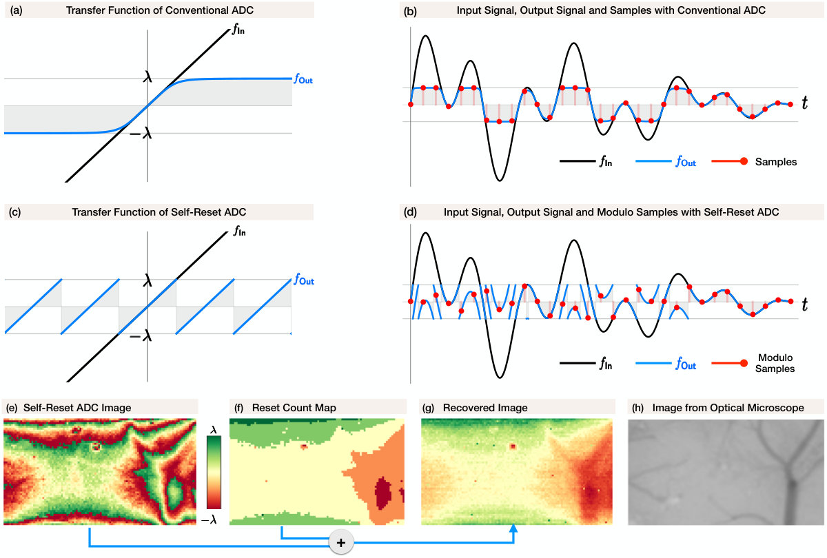 Figure 1
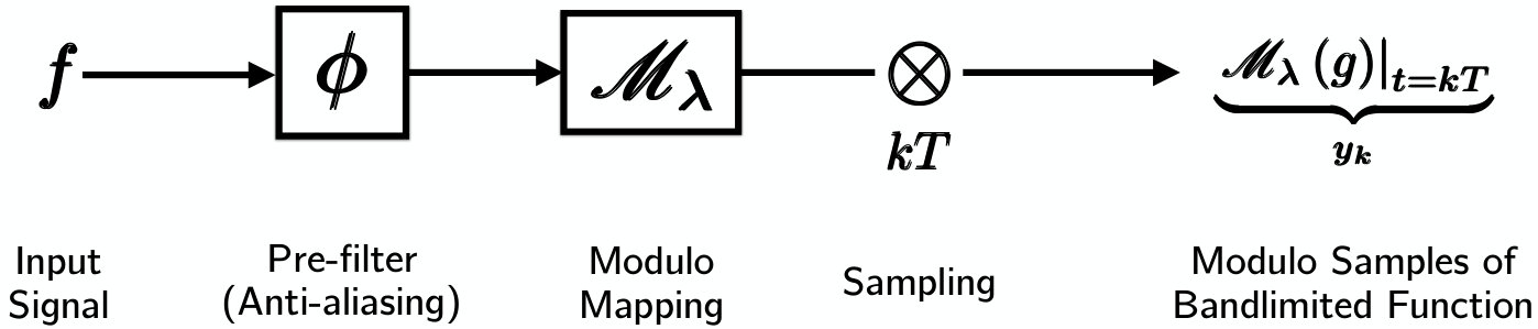 Figure 2
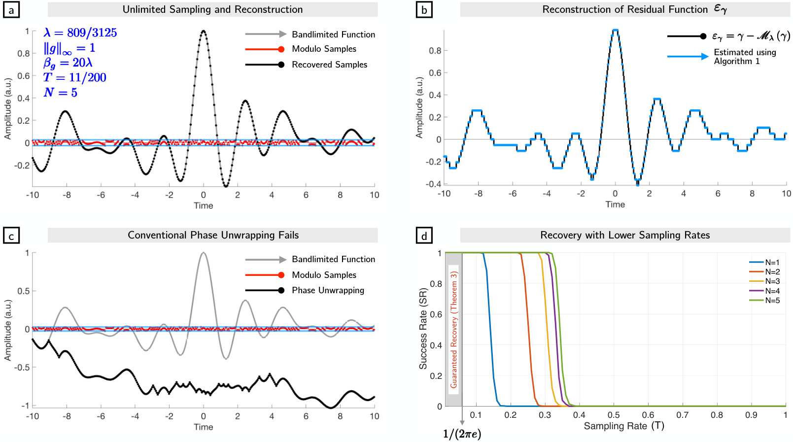 Figure 3
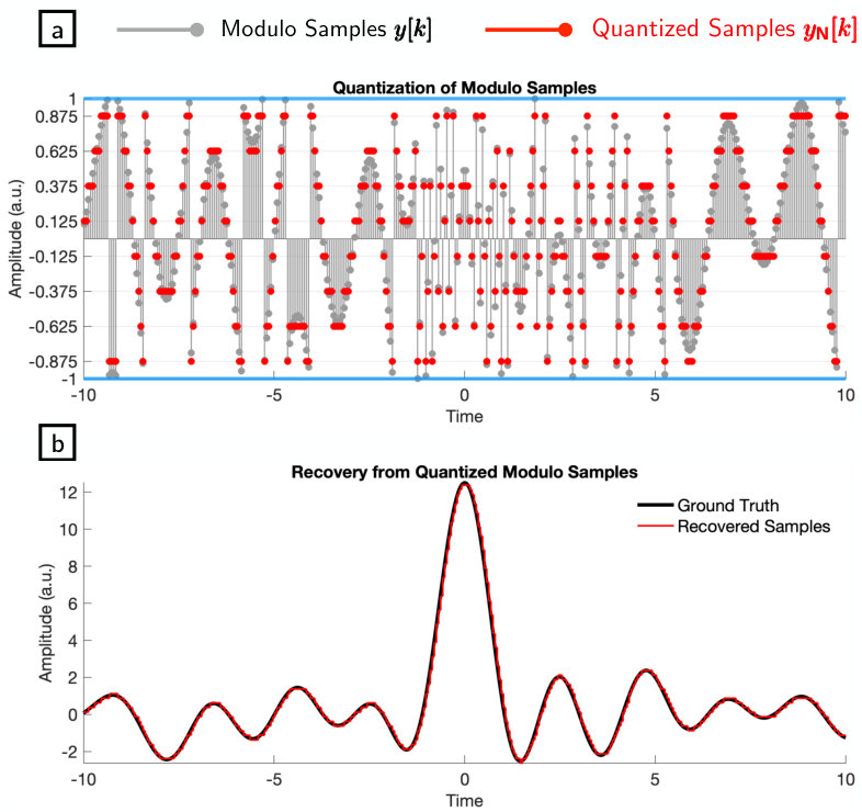 Figure 4
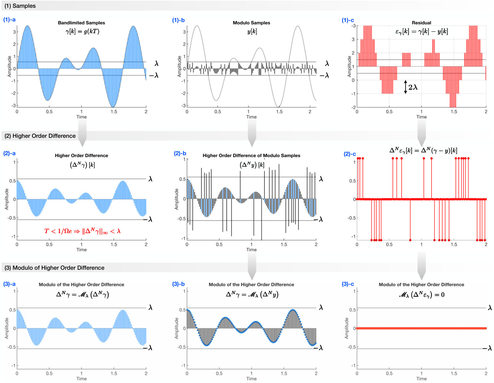 Figure 5
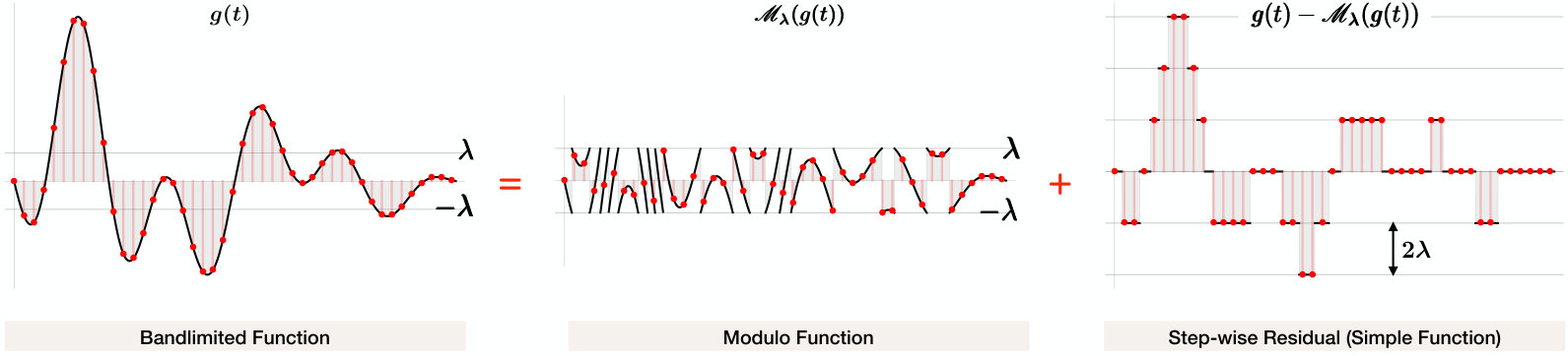 Figure 6
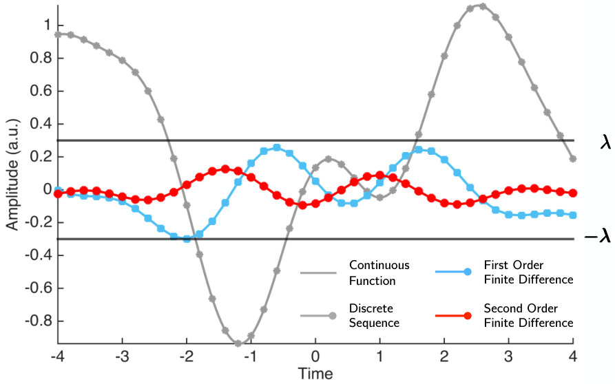 Figure 7
Peer Reviews
No public reviews on file for this paper yet. If you reviewed it on a platform where reviews are public (OpenReview, ICLR, NeurIPS, ICML), you can paste yours below so the community can read it here.
Videos
No videos yet. Explain this paper in a talk, walkthrough, or lecture? Add one.
On Unlimited Sampling and Reconstruction
Ayush Bhandari, Felix Krahmer, and Ramesh Raskar This work was presented in parts at the Intl. Conf. on Sampling Theory and Applications (SampTA), [1, 2]. A version of this work was included in [3] and led to the US Patent [4]. A. Bhandari’s work is supported by the UK Research and Innovation council’s FLF program “Sensing Beyond Barriers” (MRC Fellowship award no. MR/S034897/1). F. Krahmer acknowledges support by the German Science Foundation (DFG) in the context of the collaborative research center TR 109.A. Bhandari was with the Massachusetts Institute of Technology. He is now with the Dept. of Electrical and Electronic Engineering, Imperial College London, South Kensington, London SW7 2AZ, UK. (Email: [email protected])F. Krahmer is with the Dept. of Mathematics, Technical University of Munich, Boltzmannstraße 3, 85748 Garching/Munich, Germany. (Email: [email protected])R. Raskar is with Media Lab, Massachusetts Institute of Technology, 77 Massachusetts Ave. Cambridge 02139, MA, USA. (Email: [email protected])
Abstract
Shannon’s sampling theorem is one of the cornerstone topics that is well understood and explored, both mathematically and algorithmically. That said, practical realization of this theorem still suffers from a severe bottleneck due to the fundamental assumption that the samples can span an arbitrary range of amplitudes. In practice, the theorem is realized using so-called analog–to–digital converters (ADCs) which clip or saturate whenever the signal amplitude exceeds the maximum recordable ADC voltage thus leading to a significant information loss.
In this paper, we develop an alternative paradigm for sensing and recovery, called the Unlimited Sampling Framework. It is based on the observation that when a signal is mapped to an appropriate bounded interval via a modulo operation before entering the ADC, the saturation problem no longer exists, but one rather encounters a different type of information loss due to the modulo operation. Such an alternative setup can be implemented, for example, via so-called folding or self-reset ADCs, as they have been proposed in various contexts in the circuit design literature.
The key task that we need to accomplish in order to cope with this new type of information loss is to recover a bandlimited signal from its modulo samples. In this paper we derive conditions when perfect recovery is possible and complement them with a stable recovery algorithm. The sampling density required to guarantee recovery is independent of the maximum recordable ADC voltage and depends on the signal bandwidth only. Our recovery guarantees extend to measurements affected by bounded noise, which includes the case of round-off quantization.
Numerical experiments validate our approach. For example, it is possible to recover functions with amplitudes orders of magnitude higher than the ADC’s threshold from quantized modulo samples upto the unavoidable quantization error.
Applications of the unlimited sampling paradigm can be found in a number of fields such as signal processing, communication and imaging.
Index Terms:
Analog-to-digital conversion (ADC), approximation, bandlimited functions, modulo, Shannon sampling theory.
Contents
-
II-C The Structure of Discontinuities in Modulo Representation
-
IV-B1 Recovering Higher Order Differences from Modulo Samples
I Introduction
The interplay between the continuous and the discrete realms is at the heart of all modern information processing systems. Thus, the sampling theory inevitably finds its way in different spheres of science and engineering.
Since its early days, the topic has grown far and wide [5, 6, 7]. Researchers and practitioners have proposed a number of extensions. When we think of sampling theory, in most cases, variation on the theme arises from diversity along the time-dimension. This could be due to priors (sparsity or smoothness) or sampling architecture (uniform or non-uniform sampling grid). On the other hand, a hypothesis on the amplitude dimension leads to a different class of sampling problems, namely, level cross sampling, amplitude sampling, quantization and phaseless reconstruction. Our work falls into the latter category. In some sense, it can be seen as an amplitude analogue of the time-warped sampling theory [8], as in, our work exploits warping along the amplitude axis.
I-A The Sampling Theorem and a Practical Bottleneck
The key result of sampling theory is Shannon’s sampling theorem [7], which states that functions of bounded frequency range can be perfectly recovered from equidistant samples. To realize this theorem in practice, one uses the so-called analog–to–digital converter, henceforth ADC. Unlike the input of the sampling theorem which are assumed to be perfect samples, the output of an ADC is clipped at some fixed maximum recordable voltage; ADCs are limited by their dynamic range. This means that only values in a particular range, say, , may be recorded. We will refer to as the ADC threshold. Whenever the input signal amplitude exceeds the threshold, that is , the ADC saturates and essentially outputs . This is shown in Fig. 1 (a) and Fig. 1 (b). Such cases cannot be handled by sampling theory.
Clipping or saturation poses a serious problem in a variety of applications. For example, a camera facing the sun leads to an all white photograph which is the basis of high dynamic range photography [9]. This effect is particularly important in the context of self-driving vehicles. Scenarios such as moving out of a tunnel in the day [10] or a headlight in the line-of-sight can cause the imaging sensors to saturate. Similarly, in scientific imaging systems such as ultrasound [11], radar [12] and seismic imaging [13], strong reflections or pulse echoes blind the sensor. In communication systems, clipping results in performance degradation [14]. In the context of music, clipped sound results in high frequency artifacts [15].
Due to the pervasiveness of the clipping effect, several papers have studied this problem in different contexts (cf. [19, 11, 15, 20]) and particular emphasis has been put on audio signals (cf. [15] and references therein)—specific examples of bandlimited signals. In general, clipping of a smooth signal results in non-smooth features which in turn corresponds to high-frequency distortions in the signal. Hence, clipped or saturated signals are prone to aliasing artifacts [21].
On one hand, purely computational approaches involve de-clipping or restoration algorithms [22, 23, 19, 20, 21] with the hope of recovering lost samples under certain assumptions. Such approaches suffer from two basic drawbacks:
- •
Recovery guarantees in terms of the sampling density are largely unexplored. Ideally, the required sampling rate should be completely governed by the signal bandwidth.
- •
The mapping is discrete to discrete rather than incorporating sampling theory and following the goal of minimizing the error of the reconstructed continuous signal.
On the other hand, hardware-only approaches tackle the dynamic range problem at the ADC level [24, 25, 26]. This results in sophisticated electronic architecture that is application specific and is agnostic to the benefits offered by computational and algorithmic methods.
I-B A Solution via Modular Arithmetic
Unlike the literature discussed above which relies either entirely on computational approaches or only optimizes the hardware, our work is based on a co-design approach; we aim to overcome the dynamic range barrier by repurposing hardware in conjunction with new recovery algorithms.
The key innovation of our approach is that instead of (potentially clipped) pointwise samples of the bandlimited function, we work with folded amplitudes with values in the range . Mathematically, this folding corresponds to injecting a non-linearity in the sensing process. This amounts to,
[TABLE]
where defines the fractional part of and is the ADC threshold. Note that (1) is equivalent to a centered modulo operation since . By implementing the mapping (1), it is clear that out-of-range amplitudes are folded back into the dynamic range .
To connect this mathematical conceptualization to real world applications, we capitalize on recent advances in the imaging and sensor design technology. Indeed, ADC architectures that are moving towards the goal of folded sampling are rapidly developing. We have dedicated Section II-A to the discussion of such ADCs. In essence, the so-called self-reset [16] or folding [27] ADCs implement folding of amplitudes via (1) using electronic circuitry. We compare the transfer function of the conventional ADC with the self-reset ADC (henceforth Sr-Adc) in Fig. 1 (a) and Fig. 1 (c), respectively. Folding the amplitudes ensures that the entire range of the ADC is utilized (cf. Fig. 1 (c) and Fig. 1 (d)). To give the reader an idea of the functionality of this new breed of ADCs, we show the raw output of the prototype111We thank Sasagawa [17], Yamaguchi [18] and co-workers for providing the data which allowed us to reproduce these images. Sr-Adc arising in the context of imaging in Fig. 1 (e) and Fig. 1 (f).
While the recent decade has seen remarkable progress on the hardware aspects of the new ADCs, theoretical and algorithmic aspects has not been a major research focus and did not make their way to other fields. Current hardware literature [16, 17, 18] employs a fairly elementary approach for recovery that uses both the modulo samples and the residuals or reset counts222As per current approaches, any function (signal or image) can be written as a sum of the folded function and the reset count map. By recording both the folded function as well as the reset count map simultaneously, the original function can be recovered by a straight-forward sum of the two entities. For example, the image in Fig. 1 (g) is obtained by adding Fig. 1 (e) and (f). (see Fig. 1 (g)). This requires,
- •
complex circuitry and ADC architectures as well as,
- •
additional power and storage.
Furthermore, the feasibility of the reset count for arbitrarily small modulo thresholds has not been investigated yet.
In view of this discussion, we aim for an approach that does not suffer from these shortcomings and recovers the signal without knowledge of residuals or reset-counts. In full generality, this is a very difficult problem, which may also explain the limited progress. Namely, without further assumption on the underlying image or signal, the problem is closely related to the phase unwrapping problem, which is known to be highly ill-posed [28] and typically relies on inversion of the first-order finite difference (cf. Section I-D and Itoh’s condition.). Indeed, in both cases, one seeks to “unwrap” a discrete function representation from modulo information. Consequently, algorithms proposed for phase unwrapping also yield solution strategies for the signal unfolding problem [29, 30].
As in the case of phase unwrapping, however, these approaches suffer from strong limitations of the dynamic range (cf. Fig. 6 for a numerical comparison). For more information on the phase unwrapping problem, we refer to the literature overview in Section I-D.
An important difference, however, is that for the scenario studied in this paper, one has a considerably larger degree of control of the data entering the sensing pipeline. In particular, it is possible to sense redundant information, which in many other setups has been shown to alleviate the ill-posedness and allow for guaranteed recovery. Examples include sigma-delta quantization of bandlimited functions [31] and compressed sensing [32, 33]. In analogy to these works, our goal is to explore redundant representations that allow to overcome the limitations of the conventional viewpoint of phase unwrapping.
I-C Contributions and Overview of Results
The goal of this paper is to pose and study the inverse problem of recovering a continuous-time bandlimited function from its noisy folded samples without requiring the knowledge of residuals or reset-counts. Our key contributions are as follows:
We take a first step towards a sampling theory for modulo samples. To this end,
- •
We establish that a finite energy bandlimited function is identifiable by its modulo samples even when the sampling rate is just slightly above Nyquist.
- •
We present a sampling theorem which describes sufficient conditions for sampling and reconstruction of bandlimited functions in the context of folded samples.
- •
We show that this sampling theorem includes stability with respect to bounded noise thus covering scenarios with round-off quantization. 2.
On the algorithmic front, our sufficiency condition is complemented by a constructive recovery algorithm that is guaranteed to recover the underlying signal and is stable with respect to noise both in theory and in experiments.
Our main contribution leads to the Unlimited Sampling Theorem which is summarized below.
Theorem** (Unlimited Sampling Theorem).**
Let be a finite energy, bandlimited signal with maximum frequency and let in (1) be the modulo samples of with sampling rate {\color[rgb]{0,0,0}\mathrm{T}}. Then a sufficient condition for recovery of from is that {\color[rgb]{0,0,0}\mathrm{T}}\leqslant\frac{1}{2\Omega e} (up to additive multiples of ) where denotes Euler’s constant.
Remarkably, our theorem requires a sampling rate depending on the bandwidth only, independent of the ratio between ADC threshold, , and signal amplitude. This is why we refer to our method as unlimited sampling. Our numerical demonstrations in Section V clearly corroborate that it is possible to recover signals whose amplitude range significantly exceeds the dynamic range of the ADC under consideration, that is, .
I-D Related Problems in Other Fields and Recent Work
To put our results into context, we briefly compare and contrast topics where the modulo operation arises naturally. A disparate survey of the literature is presented below.
Phase Unwrapping. The phase unwrapping problem333We thank Prof. Laurent Jacques (UC Louvain) and Prof. Alan Oppenheim (MIT) for bringing the topic of phase unwrapping to our notice and clarifying the intricate differences with respect to sampling theory. [34, 35, 36], which finds widespread applications, specially in imaging, arises in a number of applications related to imaging (cf. [35] as well as Chapter 3 in [3]) where one only has access to a sinusoid of varying phase shift and the relevant information is encoded in these shifts, which are assumed to be varying smoothly. Due to the periodicity of the sinusoid, one can only extract this information modulo , so the goal is to recover a smooth phase function that corresponds to these observations. In this sense, the phase unwrapping problem is closely related to the problem studied in this paper, although it arises in quite a different way; the ambiguity is inherent in the sensing problem whereas we deliberately inject this non-linearity to enhance the reconstruction quality. This computational design aspect becomes important as it allows for further modifications such as the introduction of redundancy.
Given this similarity it should not come as a surprise that one of the cornerstone methods for phase unwrapping can be seen as a simplified version of the algorithm proposed in this paper. More precisely, when the max-norm of the first-order finite difference of the samples is bounded by or, , one can recover by inverting the first-order finite difference operator on the modulo sequence. This is an established result and is widely known as Itoh’s condition [34]. Please refer to Fig. 2 for a schematic explanation of Itoh’s condition and Fig. 6 for numerical comparison with our approach. Due to the redundancy via oversampling in our sensing setup, we are able to advance this method both in terms of admissible signal amplitudes and stability. 2.
Digital Communications. In the work dating back to early 1970s, Tomlinson [37] and Harashima [38] describe the use of modulo precoding444We thank Prof. Robert Gray (Boston University) who shared several historical facts regarding the role of modulo operations in the context of precoding and offering clarifications with reference to his work on modulo sigma-delta modulation that is mentioned in Section II-A. in the context of communication over channels with inter-symbol interference. In recent years, modulo operation has also been used in integer-forcing communication [39]. Although the role of such strategies in connection with sampling theory is unclear, there may be potentially interesting links for specific signal structures and reconstruction algorithms for the case of folded samples. 3.
Rate Distortion Analysis and Prediction Based Recovery. As early as in 1979, Ericson & Ramamoorthy [40] considered quantized modulo samples in the context of a source coding scheme they referred to as Modulo-PCM. Here, the authors, propose a heuristic decoder based on the Viterbi algorithm for the case of first-order Gauss-Markov processes. In early 90’s, Chou & Gray [41] studied the behaviour of quantization noise in the context of modulo sigma-delta modulation. More recently, Boufounos [42] developed a recovery scheme for modulo quantized measurements that is based on consistent reconstruction. However, all of these approaches are only feasible in limited dimensions and quite costly when the dimension is large. Our approach, in contrast, is stable and efficient and is easily scalable to a large number of samples in a mathematically guaranteed fashion. The approach in [42] can be made more practicable with the knowledge of additional side-information [43] via prediction based recovery. Following the initial ideas underlying this work as summarized in [1], a modulo sampling based simulated hardware implementation and quantization of bandlimited functions was studied by Ordentlich *et al. *in [44], again using additional side information. The authors considered oversampled representation for both single and multiple channel cases. Later, in [45], Romanov & Ordentlich studied recovery for non-quantized samples and showed that sampling faster than Nyquist rate is enough under some mild decay conditions. The side information used in [44] and [45] consists of a certain number of non-modulo samples based on which linear prediction using Chebyshev polynomials [46] can be employed to extrapolate the bandlimited function. In contrast to all these works, such side-information is not required for the method presented in this paper. This is of particular advantage when only a finite number of measurements is available, for instance, in the case of parametric signals [47, 48] as one can not expect that modulo non-linearity will leave any patch, unaffected. 4.
Modular Exponentiation. Consider the problem of computing and storing a number where are all integers. This problem frequently arises in number theory, computer science and cryptography [49]. The literature in this area focuses on without computing as the digital storage required by the former is much smaller than the latter. In this spirit, our work is similar to modular exponentiation as the ADC threshold (in analogy to ) controls the amount of information/bits required for representing the dynamic range. 5.
Contemporary Literature (2018 onwards). During the completion of this manuscript, our first work [1] was followed up in several papers. Below, we summarize the key results.
- —
Rudresh *et al. *[50] study a wavelet based algorithm for reconstruction of Lipschitz continuous functions in the context of unlimited sensing framework. 2. —
Cucuringu & Tyagi [51] investigated a more general setup based on Hölder continuous functions. They also presented a denoising approach based on a quadratically constrained quadratic program (QCQP) with non-convex constraints. 3. —
Compressed sensing of discrete-time sparse signals within the unlimited sampling architecture was investigated by Musa *et al. *in [52]. The authors developed a generalized approximate message passing approach to reconstruct discrete signals. Further bounds in context of Gaussian matrices were studied in [53]. 4. —
Unlimited sampling of continuous-time sparse signals in canonical and Fourier domain, was discussed in our works [47] and [48], respectively. 5. —
The idea of one-bit unlimited sampling was proposed by Graf *et al. *in [54]. This approach recovers high dynamic range signals from signed measurements thus adding to the functionality of the sigma-delta based ADCs. 6. —
Given modulo measurements of i.i.d samples drawn from a Gaussian distribution with unknown covariance matrix, Romanov & Ordentlich studied recovery methods in [55]. The case of known covariance matrix was covered in the work of Ordentlich *et al. *[44]. 7. —
In [56], the authors extend the idea of unlimited sensing for signals that live on a graph. To this end, the authors propose an integer programming based algorithm for recovery from modulo samples. 8. —
Modulo Radon Transform was presented in [57] and unlimited sampling based high dynamic range computed tomography was presented in [58]. 9. —
In recent works, [59, 60], the authors presented a multi-channel unlimited sampling approach in the context of sensor array signal processing.
I-E Organization of this Paper
The paper is organized as follows. In Section II, we discuss ADC architectures that lead to modulo samples. Section III is devoted to the study of uniqueness conditions. Recovery conditions and the reconstruction algorithm are presented in Section IV. Numerical examples that corroborate our theory are discussed in Section V. We conclude this work with future directions in Section VI.
I-F Notation
We use , , and to denote the set of natural numbers, integers, reals and complex numbers, respectively. We use \mathop{\vphantom{\bigcup}\mathchoice{\leavevmode\vtop{\halign{\hfil\m@th\displaystyle#\hfil\cr\bigcup\cr\cdot\crcr}}}{\leavevmode\vtop{\halign{\hfil\m@th\textstyle#\hfil\cr\bigcup\cr\cdot\crcr}}}{\leavevmode\vtop{\halign{\hfil\m@th\scriptstyle#\hfil\cr\bigcup\cr\cdot\crcr}}}{\leavevmode\vtop{\halign{\hfil\m@th\scriptscriptstyle#\hfil\cr\bigcup\cr\cdot\crcr}}}}\displaylimits to denote disjoint union of sets. Continuous functions are written as while their discrete counter-parts are represented as . The space equipped with the -norm or is the standard Lebesgue space. For instance, and denote the space of absolute and square-integrable functions, respectively. Spaces associated with sequences will be denoted by . The max-norm () of a function is defined as, while for sequences, we have, . The –order derivative of a function is denoted by . The space of –times differentiable, real-valued functions is denoted by . For sequences,
[TABLE]
denotes the finite difference and recursively applying the same yields order difference, . The Fourier transform of a function is denoted by with a natural extension to arbitrary distributions via duality. We say is -bandlimited or,
[TABLE]
where is the indicator function on domain . This includes functions with infinite energy such as a pure sine wave. When dealing with finite-energy functions, it is convenient to work with the Paley-Wiener space, . Note that for , one has . In the context of numerical computations, and denote the floor and ceiling functions.
II Sr-Adcs and Modulo Samples
II-A Background on Self-Reset ADCs
When reaching the upper or lower saturation voltage, the Sr-Adcs reset to the respective threshold. This is what allows for capturing voltage variations beyond the conventional saturation limit. This mechanism aptly justifies the name self-reset or folding ADCs which is mathematically equivalent to using the modulo mapping in (1).
As is often the case, theoretical conceptualization of such ADCs predated its practical implementation. To bring the reader up to pace with the literature, we will quickly review the key references in the area. As early as in the late 1970’s, the concept of modulo limiters was used in the context of Tomlinson–Harashima decoders [37, 38] in communication theory. Chou and Gray [41] studied the resulting quantization noise but, neither the physical realization nor their recovery properties were investigated. It was only in the early 2000’s that the physical implementation of such ADCs started to develop. One of the earliest references is due to Rhee and Joo [16] where the authors proposed the Sr-Adc in context of CMOS imagers. Interested readers are also referred to a tutorial article on folding ADCs by Kester [27] which contains historical references. In a study on quantitative characterization of ADC architectures, Kavusi and Gamal [61] note that Sr-Adcs allow for simultaneous enhancement of both dynamic range as well as the signal-to-noise ratio. We remark that the revolution around the Sr-Adcs is mainly motivated by the goal of achieving improvement on the dynamic range. This is primarily because the dynamic range of natural scenes is typically much larger than what a conventional ADC or an imaging sensor may accommodate. While HDR imaging requires several exposures, Sr-Adc based imaging is inherently HDR due to folding of amplitudes. An alternative architecture for HDR imaging via modulo operations was recently used in [28]. Beyond consumer photography [9] and autonomous vehicle navigation [10], improvement on dynamic range is important for scientific and bio-imaging. To this end, Sasagawa [17] and Yamaguchi [18] recently developed an implantable Sr-Adc for functional brain imaging.
II-B Mathematical Model for Unlimited Sampling
Thanks to the Sr-Adcs [16, 17, 18], we can repurpose the resetting capability for obtaining modulo samples without recording the reset counts (cf. Section I-B and Fig. 1 (f)). The sampling process for obtaining modulo samples of a function is outlined in the block diagram in Fig. 3. The basic principles are similar to the conventional case except for the modulo mapping. A break down of the key steps is as follows:
We start with a square-integrable function (not-necessarily bandlimited) to be sampled. 2.
Pre-filtering of with results in a low-pass approximation which is given by,
[TABLE]
Also note that since , it admits the standard sampling formula for bandlimited functions,
[TABLE]
where {\color[rgb]{0,0,0}\mathrm{T}} is the sampling rate and is the ideal low-pass filter. 3.
The bandlimited function is folded in the range via non-linear mapping (1) and results in,
[TABLE] 4.
The folded function is sampled using impulse-train, {\otimes_{k{\color[rgb]{0,0,0}\mathrm{T}}}}\stackrel{{\scriptstyle\rm{def}}}{{=}}\sum\limits_{n\in\mathbb{Z}}{\delta\left({t-k{\color[rgb]{0,0,0}\mathrm{T}}}\right)}, with sampling rate {\color[rgb]{0,0,0}\mathrm{T}}>0 yielding uniform samples,
[TABLE]
as shown in Fig. 3. 5.
When considering quantization with a budget of bits per sample, each modulo sample is rounded to the closest element in the set
[TABLE]
Note that this operation induces noise that is not following a random model, but is entry-wise bounded by , which is why our guarantee below considers bounded deterministic noise.
We plot , and modulo samples in Fig. 1.
II-C The Structure of Discontinuities in Modulo Representation
Clearly, the unlimited sampling architecture converts a smooth function into a discontinuous one. Recovering the unfolded function from scrambled, low dynamic-range, samples then boils down to patching the discontinuities together. In fact, it turns out that the discontinuities admit a structure which is critical to our cause. Every bandlimited function, continuous or discrete, can be decomposed as a sum of a modulo function and a step-wise residual that we call simple function. This is shown in Fig. 4. We elaborate on this aspect in form of the following proposition.
Proposition 1** (Modular Decomposition Property).**
Let and be defined in (1) where is a fixed, positive constant. Then, the bandlimited function admits a decomposition
[TABLE]
where and is a simple function,
[TABLE]
where \mathop{\vphantom{\bigcup}\mathchoice{\leavevmode\vtop{\halign{\hfil\m@th\displaystyle#\hfil\cr\bigcup\cr\cdot\crcr}}}{\leavevmode\vtop{\halign{\hfil\m@th\textstyle#\hfil\cr\bigcup\cr\cdot\crcr}}}{\leavevmode\vtop{\halign{\hfil\m@th\scriptstyle#\hfil\cr\bigcup\cr\cdot\crcr}}}{\leavevmode\vtop{\halign{\hfil\m@th\scriptscriptstyle#\hfil\cr\bigcup\cr\cdot\crcr}}}}\displaylimits_{m\in\mathbb{Z}}\mathcal{D}_{m}=\mathbb{R} is a partition of the real line into intervals .
Proof.
Since , by definition, we write,
[TABLE]
where (a) is due to and in (b), we use . Since, for an arbitrary function , has the form,
[TABLE]
we obtain the desired result.
This proposition is the stepping stone towards the recovery algorithm. It allows us to tackle two problems at once:
According to (5), if is known, we can recover from . In this paper we develop a method which allows for inferring from . 2.
According to (8), the fact that the amplitudes of can only be integer multiples of allows us to enforce a consistency constraint555By the consistency constraint, we mean that in presence of noise or rounding errors, we may force the amplitudes of to be on the grid of . This is implemented using (20) and step in Algorithm 1. For numerical demonstration see Section V-C. which in turn leads to a robust recovery algorithm.
We emphasize that the decomposition property of Proposition 1 offers a general purpose utility whose potential benefits are typically not exploited. For instance, phase unwrapping [34] may directly benefit from this observation. In phase unwrapping literature, one recovers from its first-order finite difference using the anti-difference. Clearly, an arbitrary smooth function has far more degrees of freedom than (8) and hence, from robustness perspective, it is more effective to enforce the simple function structure.
III On Identifiability in Unlimited Sampling
In this section, we present identifiability conditions associated with the unlimited sampling strategy. Said differently, we answer the question of what sampling density leads to unique characterization of a bandlimited function in terms of its modulo samples? The key result of this section is that any sampling rate faster than critical sampling, that is, 0<{\color[rgb]{0,0,0}\mathrm{T}}<\pi/\Omega allows for a one-to-one mapping between a bandlimited function, and modulo samples {y[k]}=\mathscr{M}_{\lambda}\left(g\left(k{\color[rgb]{0,0,0}\mathrm{T}}\right)\right). In what follows, without loss of generality, we will normalize the bandwidth such that and the critical sampling rate is {\color[rgb]{0,0,0}\mathrm{T}}=1. In working with oversampled representations, we will denote the sampling rate by, {\color[rgb]{0,0,0}\mathrm{T}_{\epsilon}}=\frac{\pi}{\pi+\epsilon},\epsilon>0 implying that 0<{\color[rgb]{0,0,0}\mathrm{T}_{\epsilon}}<1.
III-A Uniqueness of Modulo Representation
The following Lemma is used for the proof of injectivity conditions.
Lemma 1**.**
Assume that , and is some finite set. Then is uniquely characterized by its samples in {\color[rgb]{0,0,0}\mathrm{T}_{\epsilon}}\cdot(\mathbb{Z}\setminus\mathbb{L}) where {\color[rgb]{0,0,0}\mathrm{T}_{\epsilon}}=\frac{\pi}{\pi+\epsilon},\epsilon>0 is the sampling rate.
For proof of this Lemma, we refer the reader to [2]. Lemma 1 is used to prove that oversampling uniquely determines modulo samples. The formal statement is as follows.
Theorem 1** (Injectivity Theorem for Unlimited Sampling).**
Any is uniquely determined by its modulo samples on the grid {\left\{{{t_{n}}=n{{\color[rgb]{0,0,0}\mathrm{T}_{\epsilon}}}}\right\}_{n\in\mathbb{Z}}} with .
For proof of this Theorem, we refer the reader to [2]. A subsequent alternative form of proof can be found in [45].
IV Recovery Conditions and a Reconstruction Algorithm
The result of the previous section shows that any sampling rate faster than the Nyquist rate uniquely characterizes a bandlimited function in terms of its modulo samples. However, this does not yield a constructive algorithm. This section is concerned with the development of a constructive algorithm that recovers a bandlimited function from its modulo samples as defined in (4). Our algorithm is accompanied with a recovery guarantee. Akin to Shannon’s sampling theorem, our recovery guarantee purely depends on the signal bandwidth.
IV-A Overview of the Recovery Scheme
Our basic strategy for recovering functions from modulo samples is schematically explained in Fig. 5. The key observation at the heart of our approach is that finite differences commute with the modulo operation in a certain sense. With the first order difference given by, , the order difference can be obtained by recursive application of the finite-difference operator, . Starting with modulo samples (cf. Fig. 5-(1)-b), its higher order differences are given by (cf. Fig. 5-(2)-b). Under appropriate conditions, as shown in Fig. 5-(3)-b, applying the modulo operation on reduces to and we obtain the equivalence . Equivalently, the residual function is annihilated that is, . To eventually recover from , we will work towards recovery of which can be robustly estimated as it takes amplitudes on the grid of . To do so, we compute, For , this is shown in Fig. 5-(2)-c. To recover from \color[rgb]{0,0,0}{\Delta^{N}}\varepsilon_{g}, we will use the anti-difference operator defined as,
[TABLE]
followed by rounding of \mathsf{S}\left(\color[rgb]{0,0,0}{\Delta^{N}}\varepsilon_{g}\right) to the nearest multiple of which adds to the stability. Although polynomials are in the kernel of the anti-difference operator, we will develop an approach that allows us to estimate up to an unknown constant. Finally, having estimated the residual function up to an integer multiple of , we obtain the bandlimited samples by using (5). The continuous-time function is obtained by low-pass filtering the samples using (2).
IV-B Towards a Recovery Guarantee for Unlimited Sampling
Our scheme relies on conditions under which the higher order differences of the bandlimited samples are small enough in amplitude so that the modulo non-linearity has no effect on the same. To analyze how much can one shrink the amplitudes, we will begin our analysis with a bound that relates max-norm of higher order differences with its continuous-time counterpart, the derivative. Below, we summarize some well-known consequences of Taylor’s theorem and Bernšteĭn’s inequality in form of the following lemma.
Lemma 2**.**
For any and , its samples \gamma[k]\stackrel{{\scriptstyle\rm{def}}}{{=}}g(k{\color[rgb]{0,0,0}\mathrm{T}}) satisfy
[TABLE]
Furthermore, whenever is an –bandlimited function, its samples \gamma[k]\stackrel{{\scriptstyle\rm{def}}}{{=}}g\left(k{\color[rgb]{0,0,0}\mathrm{T}}\right),{\color[rgb]{0,0,0}\mathrm{T}}\leqslant\pi/\Omega satisfy,
[TABLE]
Proof.
Using Taylor’s theorem, we can write,
[TABLE]
where is the Taylor polynomial of degree around ,
[TABLE]
and the remainder of the Taylor series in Lagrange form is given by,
[TABLE]
where is some number between and . Given a sequence of samples \gamma[k]=g\left(k{\color[rgb]{0,0,0}\mathrm{T}}\right), its higher order differences use contiguous values of where,
[TABLE]
By letting to be the center of the above and hence \tau=\left(k+\frac{N}{2}\right){\color[rgb]{0,0,0}\mathrm{T}} and sampling (12) on both sides, we can now write
[TABLE]
and consequently,
[TABLE]
because annihilates polynomials of degree . Noting that and using (13), we have,
[TABLE]
where the last but one inequality is obtained by applying the Stirling’s approximation, that is, and this proves (10).
Next, we use the well known Bernšteĭn’s inequality to bound the right hand side of (10). For –bandlimited functions , the Bernšteĭn’s inequality (cf. pg. 116, [62]) asserts that,
[TABLE]
and by plugging the same in (10), we obtain (11).
IV-B1 Recovering Higher Order Differences from Modulo Samples
The result of Lemma 2 and in particular, the inequality in (11) will be the key to our proposed recovery method. By letting {\color[rgb]{0,0,0}\mathrm{T}}<1/\Omega e and choosing logarithmically in , the right hand side of (11) can be made to shrink arbitrarily, ultimately ensuring that . More precisely, assuming that we know some constant such that,
[TABLE]
a suitable choice for that satisfies {\left({{\color[rgb]{0,0,0}\mathrm{T}}\Omega e}\right)^{N}}\beta_{g}\leqslant\lambda is,
[TABLE]
For this choice of and {\color[rgb]{0,0,0}\mathrm{T}}\leqslant{\left({2\Omega e}\right)^{-1}}, (11) entails that is unaffected by the modulo operation, that is,
[TABLE]
The following proposition relates the right hand side of (15) to the modulo samples in (4).
Proposition 2**.**
For any sequence it holds that
[TABLE]
Proof.
In view of the Modular Decomposition Property, we write, to obtain where is a simple function. With the observation that
[TABLE]
we obtain,
[TABLE]
Now since in (6) take values in and the finite difference filter has integer valued coefficients, it follows that . Consequently, is in the kernel of or . Hence,
[TABLE]
which proves the result in (16).
By letting in (16), we obtain, . Combining this with (15) yields,
[TABLE]
Hence, starting with modulo samples in (4), we are able to relate the same with higher order differences of bandlimited samples .
IV-B2 Recovery of Samples from Higher Order Differences
The result of Proposition 1 yields that,
[TABLE]
where the sequence satisfies for all . Hence given modulo samples , recovering \gamma[k]=g\left(k{\color[rgb]{0,0,0}\mathrm{T}}\right) is equivalent to recovering . Thanks to Proposition 2, with in (14), we can use the relation in (15) to estimate \color[rgb]{0,0,0}{\Delta^{N}{\varepsilon_{\gamma}}} directly from the modulo samples. This is because,
[TABLE]
It now remains to recover from \color[rgb]{0,0,0}\Delta^{N}{\varepsilon}_{\gamma}. We remind the reader that \color[rgb]{0,0,0}\Delta^{N}{\varepsilon}_{\gamma}\in 2\lambda\mathbb{Z} and this massive restriction on the range of values that \color[rgb]{0,0,0}\Delta^{N}{\varepsilon}_{\gamma} can take makes the recovery procedure considerably less ill-posed than recovering from \color[rgb]{0,0,0}{\Delta^{N}{\gamma}}. Algorithmically, recursively applying the anti-difference operator in (9) and then rounding the same to the nearest multiple of , that is,
[TABLE]
recovers \color[rgb]{0,0,0}{\Delta^{N-1}}\varepsilon_{\gamma} up to an additive constant. The remaining ambiguity is due to the constant sequence being in the kernel of the first order finite difference operator. The unknown constant can again only take values in . More precisely,
[TABLE]
where is the constant sequence and . Clearly, when , the ambiguity cannot be resolved as leads to the same modulo samples. However, for , we can resolve this ambiguity. By applying to (21), we obtain,
[TABLE]
where is a linear sequence with slope . Next, observe that,
[TABLE]
where uses the modulo decomposition property (5). Furthermore, implies that and from Lemma 2, (11), we have \|{\Delta^{n-2}}\gamma{\|_{\infty}}\leqslant{\left({{\color[rgb]{0,0,0}\mathrm{T}}\Omega e}\right)^{n-2}}\beta_{g}. Hence,
[TABLE]
From the above inequality, it is clear that oversampling or {\color[rgb]{0,0,0}\mathrm{T}}<1/\Omega e keeps the max-norm of the higher order differences bounded. Using this with (23), we conclude,
[TABLE]
where,
[TABLE]
Here, the last inclusion follows as {\color[rgb]{0,0,0}\mathrm{T}}\leqslant\left(2\Omega e\right)^{-1}. Using and {\color[rgb]{0,0,0}\mathrm{T}}\leqslant\left(2\Omega e\right)^{-1}, again, we have
[TABLE]
With (25), the above inequality yields . Let us define the sequence,
[TABLE]
Setting in (24) entails,
[TABLE]
For , the right hand side in the above is an interval of length and hence only contains one integer, namely,
[TABLE]
Together with the rounding operation defined in (20), the estimate of allows us to recursively compute,
[TABLE]
where the sequence is initialized with initial condition s_{\left({0}\right)}[k]\stackrel{{\scriptstyle(\ref{eq:egy})}}{{=}}\color[rgb]{0,0,0}\Delta^{N}{\varepsilon}_{\gamma}[k]. This completes the recovery procedure which is summarized in Algorithm 1. The following theorem provides a recovery guarantee for this algorithm.
Theorem 2** (Unlimited Sampling Theorem).**
Let and {y[k]}={\left.{\mathscr{M}_{\lambda}\left({g\left(t\right)}\right)}\right|_{t=k{\color[rgb]{0,0,0}\mathrm{T}}}},k\in\mathbb{Z} in (4) be the modulo samples of with sampling rate {\color[rgb]{0,0,0}\mathrm{T}}. Then a sufficient condition for recovery of from the up to additive multiples of is that
[TABLE]
Provided that this condition is met and assuming that is known with , then choosing
[TABLE]
yields that {\left({{\color[rgb]{0,0,0}\mathrm{T}}\Omega e}\right)^{N}}{\left\|{g}\right\|_{\infty}}<\lambda and Algorithm 1 recovers from again up to the ambiguity of adding multiples of .
The proof of this Theorem is deferred to the next section (Section IV-B3), which considers the case of bounded noise. The same proof applies in the absence of noise.
IV-B3 Recovery Conditions for the Case of Bounded Noise
In this section, we consider the effect of bounded noise on the recovery procedure. More precisely, we assume that the modulo samples are affected by noise of amplitude bounded by a constant . That is,
[TABLE]
Note that due the presence of noise, it may happen that {\color[rgb]{0,0,0}y_{\eta}}[k]\not\in[-\lambda,\lambda]. Nonetheless, for below some fixed threshold, our recovery method provably recovers noisy bandlimited samples from the associated noisy modulo samples {\color[rgb]{0,0,0}y_{\eta}}[k] up to an unknown additive constant, where the noise appearing in the recovered samples is in entry-wise agreement with the one affecting the modulo samples. That is, .
Theorem 3** (Unlimited Sampling Theorem with Noise).**
Let and assume that is known with . For the dynamic range we work with the normalization .
Let the noisy modulo samples be of the form (30) with a noise bound given in terms of the dynamic range as
[TABLE]
Then a sufficient condition for Algorithm 1 with
[TABLE]
to approximately recover the bandlimited samples in the sense that it returns is that
[TABLE]
Proof.
We start by observing that the modified choice of as given in (32) yields that . Together with (11), this yields that . Similarly, the modified choice of yields that
[TABLE]
which yields via Young’s inequality and (31) that
[TABLE]
These observations now entail that even the noisy modulo measurements {\color[rgb]{0,0,0}y_{\eta}} allow for exact computation of . Indeed, we observe that
[TABLE]
Here in (a), we used Proposition 2. Equality (b) follows from (17) and (34). For (c) we again use (34) combined with the bound derived above.
We will show now by induction in that for as in (27) and as in (18). The choice then ensures that for some . As per modulo decomposition in Proposition 1, this ensures that step 5 of Algorithm 1 returns noisy bandlimited samples , that is, one recovers up to the measurement noise and an unavoidable constant ambiguity of . The result then follows from Shannon’s sampling theorem which is implemented in step 6 of Algorithm 1.
To prove that , we first note that the induction seed reduces to showing that s_{\left({0}\right)}=\color[rgb]{0,0,0}{\Delta^{N}{\varepsilon_{\gamma}}}, which holds by definition.
For the induction step, assume that for some , one has . Recall that we have derived above that for as chosen in Algorithm 1, given by (26) is the unique multiple of for which defined in (27) is a bounded sequence. Hence, combining (21) with the induction hypothesis and the observation that ceiling and floor in (27) only have an effect in case of round-off errors, we conclude that as desired.
V Numerical Experiments
In this section, we numerically verify several results linked with the topic of unlimited sampling and reconstruction. In particular, (a) we verify our sampling theorem and explore its limitations, (b) compare Algorithm 1 with Itoh’s method for phase unwrapping and (c) confirm that our approach is stable in the presence of quantization noise. These results are plotted in Fig. 6 (a)–(d) and Fig. 7 (a)–(c).
V-A Verifying the Unlimited Sampling Theorem
In order to verify our sampling theorem, we generate realizations of a bandlimited function with piecewise constant Fourier spectrum taking values chosen uniformly at random, where denotes the uniform random distribution. The bandlimited function is normalized such that . Furthermore, for each realization, we use and . We obtain modulo samples in (4) using sampling rate {\color[rgb]{0,0,0}\mathrm{T}}=\frac{11}{200}<\frac{1}{2\pi e}. There on, we use Algorithm 1 to recover bandlimited samples. Although Algorithm 1 recovers bandlimited samples up to an unknown additive constant of , we use the knowledge of ground truth to estimate this unknown constant so that we can compute the mean squared error. For each of the realizations, the samples are recovered up to machine precision ().
A specific realization of the experiment is shown in Fig. 6 (a). With and {\color[rgb]{0,0,0}\mathrm{T}}={11}/{200}, we estimate . The recovered samples are also shown in Fig. 6 (a). The mean squared error between the bandlimited samples and recovered samples in this case is . The residue function corresponding to this realization, that is , is computed using the ground truth and its estimated version which is obtained using Algorithm 1. This is shown in Fig. 6 (b). We also compare our reconstruction with the phase unwrapping method based on Itoh’s condition [34]. As explained in Fig. 2, Itoh’s condition succeeds when , which is not the case here. As shown in Fig. 6 (c), phase unwrapping based reconstruction fails.
V-B Exploring Sharpness of the Unlimited Sampling Theorem
On one hand, the injectivity condition in Theorem 1 proves that any sampling rate above the Nyquist rate guarantees unique representation of a bandlimited function in terms of its modulo samples. On the other hand, for Algorithm 1 to succeed, the sampling rate must be a factor of faster than Nyquist rate. Here we set up a demonstration that shows that Algorithm 1 succeeds even when the sampling rate is much slower than what is prescribed by Theorem 2, however, the recovery is not guaranteed. For any , we denote the critical sampling rate by {\color[rgb]{0,0,0}\mathrm{T}_{\sf{Shannon}}}=1 and the corresponding sampling rate prescribed by the unlimited sampling theorem is {\color[rgb]{0,0,0}\mathrm{T}_{\sf{US}}}=1/2\pi e. We consider modulo samples acquired with , so the theorem is valid for all orders . To assess the sharpness of Theorem 2, we use realizations of randomly generated bandlimited functions with . Each realization is then sampled with sampling rate {\color[rgb]{0,0,0}\mathrm{T}}=0.01,\ldots,{\color[rgb]{0,0,0}\mathrm{T}_{\sf{Shannon}}} in steps of and we set . For sampling rates beyond the applicability of the theorem, that is, {\color[rgb]{0,0,0}\mathrm{T}}>{\color[rgb]{0,0,0}\mathrm{T}_{\sf{US}}}, we run Algorithm 1 for each of realizations by varying from to . Then for each combination of {\color[rgb]{0,0,0}\mathrm{T}} and , we compute the success rate which is defined as the fraction of trials in which the algorithm reconstructs up to machine precision (in the sense of mean-squared error). As shown in Fig. 6 (d), indeed the recovery is possible even when {\color[rgb]{0,0,0}\mathrm{T}}\in\left({\color[rgb]{0,0,0}\mathrm{T}_{\sf{US}}},{\color[rgb]{0,0,0}\mathrm{T}_{\sf{Shannon}}}\right). Furthermore, higher order differences extend recover to smaller over-sampling factors, but there seems to be a minimum oversampling rate around {\color[rgb]{0,0,0}\mathrm{T}}=0.4 above which the algorithm always fails for the chosen value of .
V-C Quantization and Bounded Noise
As discussed in Section IV-B3, Theorem 3 provides recovery guarantees in the presence of bounded noise. A main motivation for this noise model is that it includes the error caused by round-off quantization as in Section II-B, Step 5. In Fig. 7 we illustrate the recovery guarantees for –bit quantized modulo samples. That is, each modulo measurement is rounded to the closest element of
[TABLE]
In other words, the quantized measurements are incurring quantization noise . In the experiment, we use a bandlimited function with and . As before, {\color[rgb]{0,0,0}\mathrm{T}}={11}/{200} with and we set . The experiment shows that our method is even more robust than predicted by Theorem 3: despite the quantization noise , Algorithm 1 recovers the underlying (noisy) bandlimited samples which are shown in Fig. 7 (b). The reconstruction mean squared error (MSE) between and its estimate (using Algorithm 1) is is observed to be which is the same as the MSE between and {\color[rgb]{0,0,0}y_{\eta}} and much smaller than the MSE of incurred with -bit quantization of non-modulo samples.
VI Conclusion
VI-A Summary of Results
In this work, we have described a new sensing and recovery scheme that overcomes the dynamic range barrier fundamental to digital sensing and sampling theory. Our approach harnesses a co-design between hardware and algorithms. On the hardware front, a modulo non-linearity injected in the sensing process scrambles high-dynamic-range information into low-dynamic range samples. Theorem 1 addresses the question of uniqueness; a bandlimited function is uniquely characterized by its modulo samples provided that the sampling rate is faster than critical sampling density. On the algorithmic front, given modulo samples of an -bandlimited function, the sampling rate {\color[rgb]{0,0,0}\mathrm{T}}\leqslant 1/\left(2\Omega e\right) guarantees recovery. This Unlimited Sampling Theorem is formally stated in Theorem 2; stability with respect to quantization noise and other bounded noise is established in Theorem 3. The proposed reconstruction approach hinges on the observation that the modulo and the (higher-order) difference operators commute in a certain sense.
VI-B Future Directions
Implementation Issues Implementing our approach in practice remains an integral aspect of future research. In particular, we are working to design computational techniques to address inaccuracies and instabilities arising in the implementation of our techniques in hardware. We are currently exploring such instabilities in the context of a prototype ADC. Important challenges include timing jitter and that our sensing pipeline requires ADCs without anti-aliasing filter, which makes them more sensitive to noise. For this reason, noise control needs to be implemented in alternative ways. 2.
Wider Classes of Signals and Function Spaces A natural question to ask is how our results can be extended to a wider class of signals such as smooth functions (shift-invariant spaces), sparse signals, parametric classes of signals among others. Some partial answers are provided in [50, 51, 52, 53, 47, 48] but this is an open area with several unanswered questions. Unlimited sampling in spline-spaces was recently discussed in [63]. Another interesting variation is to consider multi-dimensional signal models defined on arbitrary lattices, such as [64]. 3.
Wider Classes of Inverse Problems The unlimited sensing framework leads to a new class of inverse problems due to the modulo non-linearity. It can be further combined with several interesting inverse problems where dynamic range poses a natural limitation. More generally, one may consider where is some operator. For instance, using as the Radon Transform, recently we have introduced the Modulo Radon Transform in the context of high-dynamic-range computed tomography [57]. 4.
New Sampling Architectures The unlimited sensing framework can be combined with different sampling architectures. For instance, in [54], one-bit recovery is proposed based on the sigma-delta modulation scheme. Similarly, this work can be combined with multi-channel acquisition approaches which naturally find applications in imaging, for example, time-of-flight imaging [3] and our upcoming work on direction-of-arrival estimation from modulo samples [59]. 5.
Robustness to Outliers While our results yield recovery for bounded noise, our approach is not yet stable with respect to outliers. Given the redundancy of the data, we expect that it will be possible to address this issue and, subsequently, study unbounded noise models such as Gaussian and Poissonian noise.
The reference list from the paper itself. Each links out to its DOI / PubMed record.
- 1[1] A. Bhandari, F. Krahmer, and R. Raskar, “On unlimited sampling,” in Intl. Conf. on Sampling Theory and Applications (Samp TA) , Jul. 2017.
- 2[2] A. Bhandari and F. Krahmer, “On identifiability in unlimited sampling,” in Intl. Conf. on Sampling Theory and Applications (Samp TA) , Jul. 2019.
- 3[3] A. Bhandari, “Sampling time-resolved phenomena,” Ph.D. dissertation, Massachusetts Institute of Technology, 2018.
- 4[4] A. Bhandari, F. Krahmer, and R. Raskar, “Methods and apparatus for modulo sampling and recovery,” US Patent US 10 651 865B 2, May, 2020.
- 5[5] P. L. Butzer and R. L. Stens, “Sampling theory for not necessarily band-limited functions: A historical overview,” SIAM Rev. , vol. 34, no. 1, pp. 40–53, Mar. 1992.
- 6[6] A. I. Zayed, Advances in Shannon’s Sampling Theory . CRC Press, 1993.
- 7[7] M. Unser, “Sampling–50 years after Shannon,” Proc. IEEE , vol. 88, no. 4, pp. 569–587, Apr. 2000.
- 8[8] D. Cochran and J. J. Clark, “On the sampling and reconstruction of time-warped bandlimited signals,” in IEEE Intl. Conf. on Acoustics, Speech and Sig. Proc. (ICASSP) , Apr. 1990.