A non-iterative method for electrical property tomography based on a simple formula
Victor Palamodov

TL;DR
This paper introduces a non-iterative, analytic formula-based method for reconstructing electrical properties from MRI data, simplifying the process by avoiding iterative algorithms.
Contribution
It presents a novel, exact analytic approach for electrical property tomography using harmonic electromagnetic field data at Larmor frequency.
Findings
Provides a simple, non-iterative reconstruction formula
Offers a geometric method for acquiring the full inductive field
Enhances efficiency and accuracy of electrical property imaging
Abstract
A non-iterative method of reconstruction is proposed from data of MRI system and of a harmonic electro-magnetic field at Larmor frequency. The method is based on the exact analytic formula for the contrast source function. A geometric method for acquisition of the full inductive field is discussed.
Click any figure to enlarge with its caption.
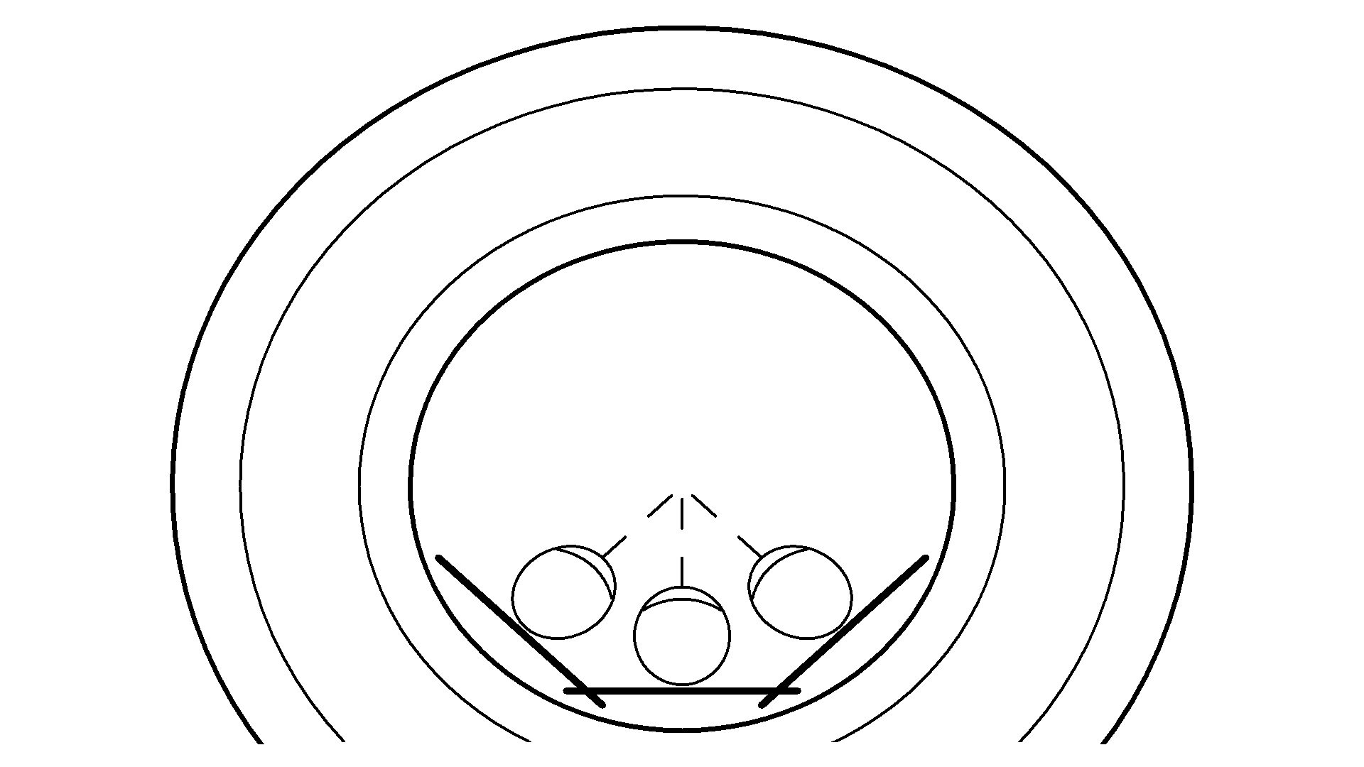 Figure 1
Peer Reviews
No public reviews on file for this paper yet. If you reviewed it on a platform where reviews are public (OpenReview, ICLR, NeurIPS, ICML), you can paste yours below so the community can read it here.
Videos
No videos yet. Explain this paper in a talk, walkthrough, or lecture? Add one.
Taxonomy
TopicsElectrical and Bioimpedance Tomography · Advanced MRI Techniques and Applications · Atomic and Subatomic Physics Research
A non-iterative method for electrical property tomography based on a simple formula
Victor P. Palamodov
Tel Aviv University
**Abstract **A non-iterative method of reconstruction is proposed from data of MRI system and of a harmonic electro-magnetic field at Larmor frequency. The method is based on the exact analytic formula for the contrast source function. A geometric method for acquisition of the full inductive field is discussed.
**Key words: **contrast source function, Helmholtz operator, transmit magnetic field, acquisition geometry
MSC 2010: 35Q61 65Z99
1 Introduction
Electrical properties tomography (EPT) is a noninvasive reconstruction technique for retrieving electrical properties (conductivity and permittivity) of biological tissue from magnetic fields generated by radio frequency coils in a magnetic resonance imaging scanner. The electric properties of tissue are of great interest, since these properties can be used to aid the discrimination of cancerous tissue from benign tissue and characterize various kinds of pathological tissue of human body [4], [8]. The main benefits of EPT over other reconstruction modalities is that it uses the Larmor frequency fields of an MRI system, which can penetrate biological tissues and it does not make use of surface electrode mounting, current injection or additional hardware.
The method called now EPT was proposed by Haacke et al. [1]. The first application of this method was done by Wen [2] who used an approximation for the contrast source function (CSF). Song and Seo [6] reduced reconstruction of admittivity to solution of an elliptic equation under assumption in terms of field. See also [9] for an explicit construction. Ammari *et al [7] *studied the problem in terms of the quasilinear system of differential equations. In [10] a survey of local methods of reconstructions is given. C van den Berg et al [11] developed the iterative method of determination of the CSF of an object making use of a global integral approach. Arduino *et al [12] applied the iterative conjugate gradient method (1000 steps). We describe here a non-iterative algorithm *for retrieving CSF which is based on the exact global formula. This is the first algorithm of this kind so far.
2 Basic equations
We assume that the conductivity and permittivity are isotropic at the angular Larmor frequency and ignore spatial permeability variations , since they are considered small for biological tissue. Let be an object domain in the MRI scanner that is disjoint of the antenna (coil) generating the RF wave. The total time harmonic electromagnetic field in can be written in the form \left\{E\exp\left(i\omega t\right),H\exp\left(i\omega t\right)\right\}\where
[TABLE]
is the incident and \left\{E^{sc},H^{sc}\right\}\the scattered fields due to the presence of the object. Following to van der Berg et al [8] we use the integral representations
[TABLE]
[TABLE]
for the scattered fields where , is the permittivity in vacuum and
[TABLE]
is the vector potential and
[TABLE]
is the scalar Green’s function for the Helmholtz operator in 3D background medium. The contrast source function is defined as
[TABLE]
where admittivity is the per meter admittance. Conductivity and permittivity are profiles of the object, \Omega\ is a domain that contains the support of
3 Evaluation of the contrast function
We write the electric and magnetic fields as first order differential forms
[TABLE]
Hodge star operator acts linearly on differential forms on by the rule ([13], p.15)
[TABLE]
where \alpha,\beta\are arbitrary differential forms in \mathbb{R}^{3}\of equal degree and \left\langle,\right\rangle\means the natural scalar product of the forms. The dual differential is defined by and Laplace operator commutes with and \mathrm{d}^{\ast}.\
Theorem 1
Let be a domain in disjoint of the RF antenna. If the fields and are known then the contrast source function can be found in by
[TABLE]
if the denominator does not vanish.
Corollary 2
We have
[TABLE]
Note that since and \mathbf{H}^{\ast}\wedge\mathbf{E}=\left\langle\mathbf{H,E}\right\rangle=0.\
**Remark. **Equation
[TABLE]
is mentioned* *by Seo [6] and attributed to Nachman et al [3].
Proof of Theorem 1**. **
Lemma 3
Let be a compact set in that can be contracted to a point in itself. For any k\geq 1,\and arbitrary closed differential -form on , there exists a -form on \Omega\such that\ \mathrm{d}b=a\on
For a proof see ”Converse of the Poincaré lemma” [13], p.29.111We may assume that coefficients of and of b\are distributions since will not appear in the final formula..
Note that equation (5) does not depend on \Omega.\Therefore we may assume that is a compact set with smooth boundary in \mathbb{R}^{3}\that fulfils the condition of Lemma 3.
Lemma 4
The system of equations for a 1-form
[TABLE]
has a solution defined on \Omega.\There exists a function on such that
[TABLE]
Proof. Form has bounded coefficients and fulfils the Gauss law on \Omega.\By Lemma 3 there exists 1-form on \Omega\that satisfies . Consider Dirichlet problem
[TABLE]
for a function on \Omega.\To solve it we define the function on that is equal to -\mathrm{d}^{\ast}C_{0}\on and on the complement to Set where is the kernel (4) with k=0.\Differential form fulfils (8) since
[TABLE]
Equation (2) implies
[TABLE]
where and is the vector potential (3). By (8) we have Again, by Lemma 3 there exists a function on such that and (9) follows.
[TABLE]
since \nabla\nabla\cdot\ =\mathrm{dd}^{\ast}\where. This yields
[TABLE]
By (9) we have
[TABLE]
since \nabla\nabla\cdot\mathrm{d}g=\mathrm{dd}^{\ast}\mathrm{d}g=\Delta\mathrm{d}g.\Apply Helmholtz operator to both parts and get
[TABLE]
since
[TABLE]
where is the delta-function on . Dividing by we obtain
[TABLE]
where \theta\doteqdot\chi/\left(1-\chi\right)\hence
[TABLE]
Differential operators and commute, therefore
[TABLE]
Multiplying by form we kill the term with
[TABLE]
By (9)\ \mathrm{d}C=\mathrm{d}A_{0}=B^{\ast},\hence
[TABLE]
which yields
[TABLE]
Finally
[TABLE]
and (5) follows.
4 Acquisition geometries
Any acquisition geometry should be rich enough to guarantee reconstruction of field on Let be an euclidean positively oriented coordinate system on the physical space such that the static magnetic field has the form in this system. The field
[TABLE]
is called positively rotating part of B\or transmit field. Several methods (sequences) are known that provide positively rotating part of a magnetic field for ex. [5]. According to [4] the ”negatively rotating” part can not be determined in this way.** **The asymmetric role of coordinates and in (10) is defined with respect to coordinate which means that the coordinate system is positively oriented. Note that the orientation is indispensable feature of the Maxwell system which is illustrated by Maxwell’s right hand rule. It follows that such measurements of the transmit field can be made for any positively oriented coordinate system that is in the system obtained by rotation of the system
**1. **The simple acquisition geometry for magnetic field is to fix the body on the bed and rotate both around the central axis that is parallel to the bed. Let be the laboratory euclidean positively oriented (left-handed) system of coordinates, and let be the positively oriented system of coordinates that are constant on the bed and the body when rotating that is
[TABLE]
where is the rotation angle see Fig.1.
Write magnetic field B\left(\varphi\right)=\beta\by means of both coordinate systems.
[TABLE]
and note that the body components of of this field do not depend on \varphi.\Keeping in view that
[TABLE]
we obtain
[TABLE]
Suppose that measurements of the transmit field are available for \varphi=-\psi,0,\psi\and consider system of linear equations
[TABLE]
The solution exists and is unique for any
[TABLE]
hence magnetic form is uniquely reconstructed by (11). Now we can apply (5) to the fields and
**2. **Another geometry for scanning a body is as follows: the bed with the body rotating in a tilted plane around the center in field. Let be the constant tilting angle and e_{3}=\left(0,-\sin\alpha,\cos\alpha\right).\For any the vectors
[TABLE]
and e_{3}\form the orthogonal frame since and belong to the plane P\through the origin orthogonal to . This frame is a positively oriented. Functions
[TABLE]
are euclidean coordinates that are constant on . To express the transmit field (10) by means of the body coordinates we write
[TABLE]
and substitute in (11). This gives
[TABLE]
and
[TABLE]
Evaluating the transmit field for we obtain the system like (12) for unknown functions that do not depend on The determinant of this system equals
[TABLE]
where It does vanish if and \varphi_{ij}\neq 0.\It follows that for arbitrary , arbitrary different angles \varphi_{i},\ ,\functions are uniquely determined form data of fields
Algorithm for computation of Contrast source function
-
Make three measurements of the transmit field according to geometry 1 or 2.
-
Calculate the field in the coordinate system of the body. and set
-
Apply (5) to the fields and and calculate the quotient as the function \chi\of the body coordinates\ \xi,\eta,\zeta.\
The reference list from the paper itself. Each links out to its DOI / PubMed record.
- 1[1] Haacke E, Petropoulos L S, Nilges E W, and Wu D H 1991 Extraction of conductivity and permittivity using magnetic resonance imaging, Phys. Med. Biol. 36 723
- 2[2] Wen H 2003 Noninvasive quantitative mapping of conductivity and dielectric distributions using RF wave propagation effects in high-field MRI Proc. SPIE 5030 471–477
- 3[3] Nachman A, Wang D, Ma W, and Joy M 2007 A local formula for inhomogeneous complex conductivity as a function of the RF magnetic field Proc. Intl. Soc. Mag. Reson. Med. 15.
- 4[4] Katscher U et al 2009 Determination of electric conductivity and local SAR via B 1 1 {}_{\text{1}} mapping IEEE Trans. Med. Imag. 28 1365–1374
- 5[5] Sacolick L I, Wiesinger F, Hancu I and Vogel M W 2010 B 1 1 {}_{\text{1}} -Mapping by Bloch-Siegert Shift”, Magnetic Resonance in Medicine 63 1315-1322
- 6[6] Song Y and Seo J K 2013 Conductivity and permittivity image reconstruction at the Larmor frequency using MRI SIAM J. Appl. Math. 73, N 6 2262-2280
- 7[7] Ammari H, Kwon H, Lee Y, Kang K, and Seo J K (2015) Magnetic resonance-based reconstruction method of conductivity and permittivity distributions at the Larmor frequency Inverse Problems 31 105001
- 8[8] Kim S Y, Shin J, Kim D H, et al . 2016 Correlation between conductivity and prognostic factors in invasive breast cancer using magnetic resonance electric properties tomography (MREPT)”. Eur. Radiol . 26 2317–2326