Three loop QCD corrections to heavy quark form factors
J. Ablinger, J. Bl\"umlein, P. Marquard, N. Rana, C. Schneider

TL;DR
This paper introduces an algorithm for solving coupled differential equations in perturbative QCD, enabling the calculation of three-loop heavy quark form factors with improved efficiency and precision.
Contribution
The paper presents a novel algorithm for solving coupled linear differential systems in quantum field theory, applied here to compute three-loop heavy quark form factors.
Findings
Successfully computed master integrals for three-loop form factors
Extended the method to include light quark contributions
Enhanced the accuracy of perturbative QCD calculations
Abstract
Higher order calculations in perturbative Quantum Field Theories often produce coupled linear systems of differential equations which factorize to first order. Here we present an algorithm to solve such systems in terms of iterated integrals over an alphabet the structure of which is implied by the coefficient matrix of the given system. We apply this method to calculate the master integrals in the color-planar and complete light quark contributions to the three-loop massive form factors.
Click any figure to enlarge with its caption.
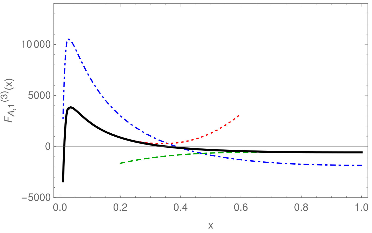 Figure 1
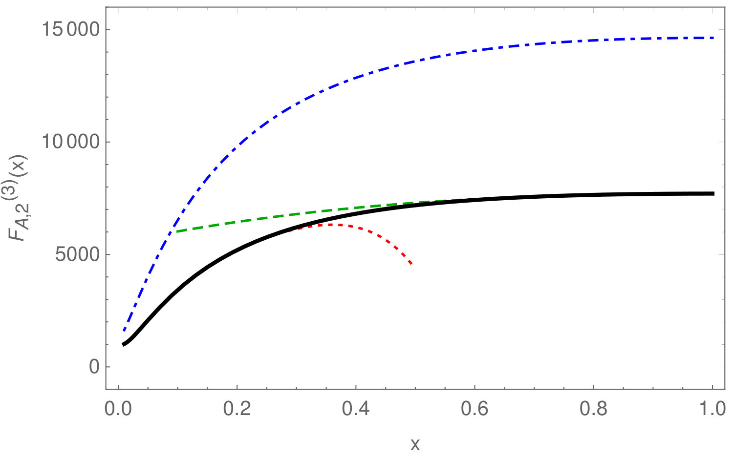 Figure 2
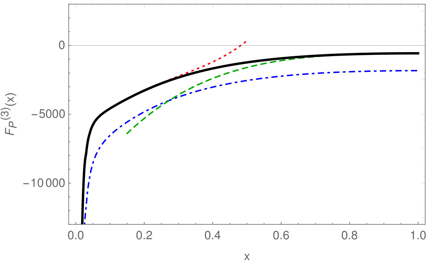 Figure 3
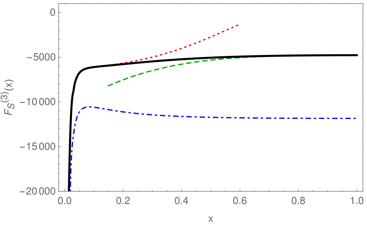 Figure 4
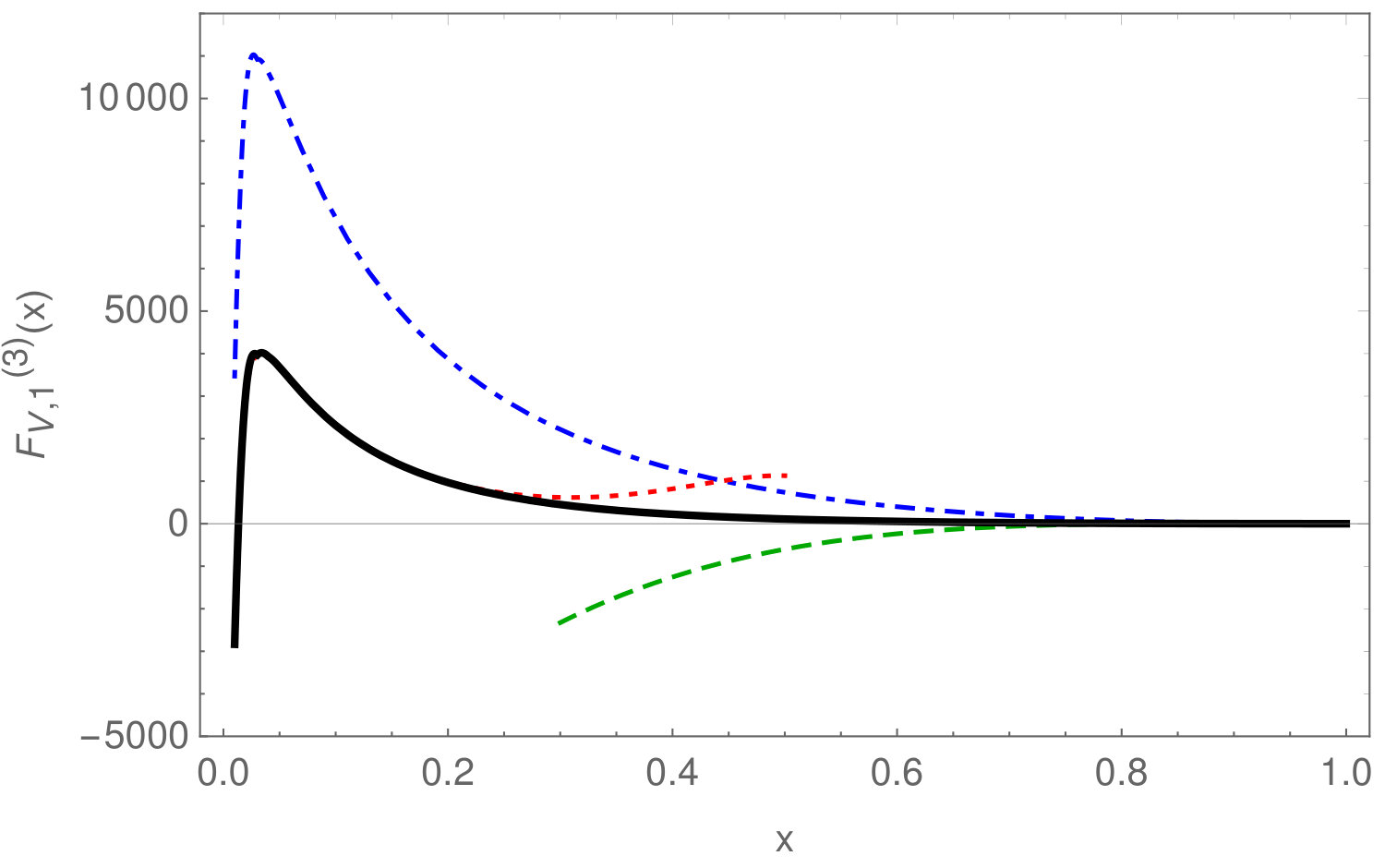 Figure 5
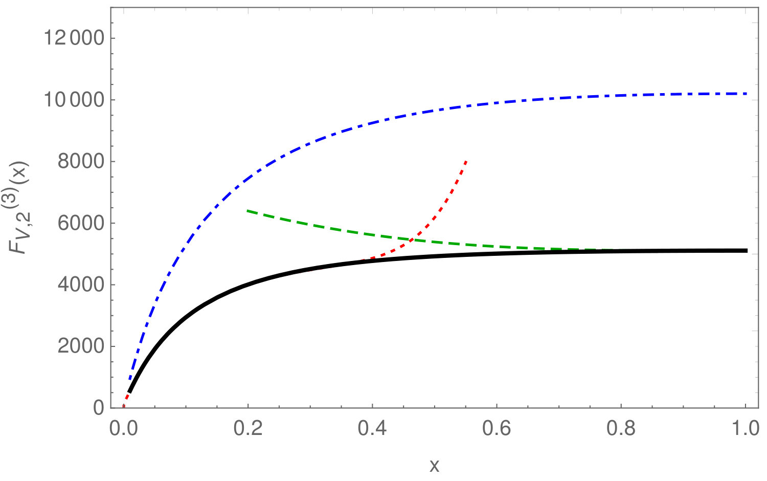 Figure 6
Peer Reviews
No public reviews on file for this paper yet. If you reviewed it on a platform where reviews are public (OpenReview, ICLR, NeurIPS, ICML), you can paste yours below so the community can read it here.
Videos
No videos yet. Explain this paper in a talk, walkthrough, or lecture? Add one.
DESY 19–078, DO-TH 19/06
Three loop QCD corrections to heavy quark form factors
J. Ablinger1
J. Blümlein2
P. Marquard2
N. Rana2,3
C. Schneider1
1RISC, Johannes Kepler University, Altenbergerstraße 69, A-4040, Linz, Austria
2DESY, Platanenallee 6, D-15738 Zeuthen, Germany
3INFN, Sezione di Milano, Via Celoria 16, I-20133 Milano, Italy [email protected]
Abstract
Higher order calculations in perturbative Quantum Field Theories often produce coupled linear systems of differential equations which factorize to first order. Here we present an algorithm to solve such systems in terms of iterated integrals over an alphabet the structure of which is implied by the coefficient matrix of the given system. We apply this method to calculate the master integrals in the color–planar and complete light quark contributions to the three-loop massive form factors.
1 Introduction
Higher order calculations in perturbative Quantum Field Theories often produce coupled linear systems of differential equations which factorize to first order. Through the integration-by-parts identities (IBP) [1, 2], the Feynman integrals appearing in a scattering amplitude can be mapped to a smaller set of integrals, the master integrals (MIs). One method to solve these integrals is the method of differential equations [3, 4, 5, 6], where one differentiates the MIs with respect to a kinematic invariant and obtains such a coupled linear system of differential equations in which we are interested in. Such an algorithm was constructed earlier in [6, 7] in the case of a system of difference equations. Here we summarize the algorithm, presented in [8], operating on uni-variate systems of differential equations, which factorize to first order. In the cases where the systems do not factorize to first order, elliptic and even more involved structures appear, cf. e.g. [9, 10, 11, 12, 13, 14, 15, 16, 17]. Our algorithm works for any basis of master integrals, while in the one in [5] a special basis is required.
As an example, we employ this method to compute the set of MIs which appear in the color–planar and complete light quark non–singlet three-loop contributions to the heavy-quark form factors for different currents, namely the vector, axial-vector, scalar and pseudo–scalar currents. These form factors are of phenomenological importance. Being the heaviest particle of the Standard Model (SM), the top quark plays an important role in comprehending the electro-weak symmetry breaking (EWSB). Consequently, many observables like the inclusive production cross section of a pair of top quarks, the forward–backward asymmetry, etc., draw attention in the post era of the Higgs boson discovery. These form factors are basic building blocks of many such observables. The two-loop QCD contributions to these massive form factors were first computed in [18, 19, 20, 21]. Later in [22], an independent computation was performed for the vector form factors, including the terms, where is the dimensional regularization parameter in space-time dimensions.
In [23], the two-loop QCD contributions up to for all massive form factors were calculated. At the three-loop level, the color-–planar contributions to the vector form factors have been computed in [25, 24] and the complete light quark contributions in [26]. Using the method described here, we have calculated both the color–-planar and complete light quark contributions to the three–loop form factors for the axial–vector, scalar and pseudo-scalar currents in [27] and for the vector current in [8], where a detailed description of the present method along with an example is presented. In a parallel calculation, the same results have been obtained in [28]. The asymptotic behavior of these three–loop form factors has been studied in [29, 30].
2 Description of the method
We consider a set of MIs within the same topology. The MIs are functions of the space–time dimension and the Landau variable defined by
[TABLE]
Here is the virtuality of the boson and denotes the heavy quark mass. One obtains an system of coupled linear differential equations by performing the derivative with respect to of each of the MIs followed by the IBP reduction,
[TABLE]
Here the matrix consists out of entries from the rational function field (or equivalently from ) where is a field of characteristic [math]. The inhomogeneous part contains MIs which are already known. In simple cases, turns out to be just the null vector. For more involved cases, we assume that each entry is expanded111In the following does not denote the th derivative of . into a Laurent series in in terms of iterated integrals
[TABLE]
To proceed, we assume that the unknown integrals can be expanded into a Laurent series in
[TABLE]
We first apply Zürcher’s algorithm [31, 33, 32, 34] (or a variant of it), implemented in the package OreSys [35], leading to a single differential equation which is then analyzed with HarmonicSums [37, 38, 39, 41, 42, 36, 40, 43, 44] for first order factorization.
The MIs can be distinguished sector–wise, where the maximal set of non–vanishing propagators in a single Feynman graph defines a sector and corresponding subsets define the sub-sectors. On the other hand, a derivative can only introduce the inverse of a new propagator. Hence, the differential equation of a MI can contain integrals from the same sector or its sub–sectors. Thus, organizing the MIs in such a way that MIs with less number of propagators are kept at the bottom of the list, provides an upper–block–triangular form of , i.e. the diagonal elements of are square matrices of rank one or more. Each such square matrix represents a completely coupled set of MIs and we call them sub–systems of . Due to such an arrangement of the system, we can now solve it in a bottom–up approach, i.e. we first solve the last coupled sub–system, having no dependence to the other MIs and work upwards in the next step. Below we present how we solve the sub–systems.
I. Let us consider integrals which constitute a coupled sub–system,
[TABLE]
where and are respective parts of and and hence have similar expansions in . Now we exploit the fact that for a certain topology and kinematics an integral has a definitive pole structure with a fixed order () of the highest pole, as e.g. the integrals arising in three–loop heavy quark form factors can have at most a pole. Keeping that in mind, we plug in Eq. (4) into Eq. (5), perform the series expansion in and obtain the coefficient of as follows
[TABLE]
II. Now we try to solve the sub–system order by order in . To accomplish that we start with the coefficient of the leading pole . The corresponding sub–system is
[TABLE]
To solve Eq. (7), a natural first step is to reduce this system to a higher order linear differential equation. We refer to this procedure as ‘uncoupling’. By using OreSys, we obtain
[TABLE]
Here are rational functions in and consists of contributions from and its derivatives. OreSys also provides the additional relations for the remaining integrals , in terms of linear combinations of and its derivatives:
[TABLE]
with and . We remark that the uncoupling may find several linear differential equations for several unknowns. However, the sum of the order of all the linear differential equations is . For simplicity we assume in the following that only one linear differential equation for is produced.
III. Now we consider the homogeneous solutions of Eq. (8). The differential equation can be factorized at first order as
[TABLE]
with being rational functions in by using algorithms from [45, 46, 47]. We find the d’Alembertian solutions , (see [8] for details) for the homogeneous part of Eq. (8) in terms of iterative integrals. In our application to the three–loop massive form factors, the alphabet is
[TABLE]
The arising iterative integrals in our application can be simplified to the harmonic polylogarithms (HPLs) [48] and cyclotomic HPLs [36]. We also note here that to fix the boundary condition of the differential equations, one needs to evaluate these iterative integrals at a particular value of , say which resulted in the example on hand into multiple zeta values (MZVs) [49] and cyclotomic constants [50, 51, 36, 52]. In [53], PSLQ [54] was used to conjecture relations beyond those known from [50, 51, 36, 52].
IV. The general solution () including the inhomogeneous part can now be easily given by the method of variation of constants in terms of iterative integrals as
[TABLE]
where is the Wronskian of the linear differential equation Eq. (8) and is given by
[TABLE]
V. Next we use the general solution for , plug it into Eq. (9) for and obtain solutions for the rest of the integrals and obtain at .
VI. Now we consider the next order () in the -expansion. We use the solution of in terms of iterative integrals and plug it into Eq. (6) for . Thus we obtain a new system of the form Eq. (7) for the -coefficient . Then the above procedure is repeated. From Eq. (6) it is evident that the homogeneous solution at each order remains same. The only changes happen to the inhomogeneous functions . As a consequence, we can reuse the already available homogeneous solutions and just need to compute in Eq. (12) with the updated function . In Ref. [8] the method has been illustrated by a detailed example.
3 Application to the massive form factors
We consider the decay of a virtual massive boson, which can be a vector (), an axial-vector (), a scalar () or a pseudo-scalar () of momentum , into a pair of heavy quarks of mass , momenta and and color and , through a vertex , where and . The general form of the amplitudes can be written as
[TABLE]
Here and are the bi–spinors of the quark and the anti–quark, respectively, with . and are the Standard Model (SM) coupling constants for the vector, axial-vector, scalar and pseudo-scalar, respectively; denotes the SM vacuum expectation value of the Higgs field, with the Fermi constant . More details can be found in [23]. The ultraviolet (UV) renormalized form factors () are expanded in the strong coupling constant as follows
[TABLE]
The form factors can be obtained from the amplitudes by multiplying appropriate projectors as given in [23] and performing the trace over the color and spinor indices. and are the numbers of light and heavy quarks, respectively.
The computational procedure of the three–loop massive form factors are outlined in Refs. [23, 27]. As usual the packages QGRAF [55], Color [56], Q2e/Exp [57, 58] and FORM [59, 60] have been used to generate the Feynman diagrams, calculate their color structure and to perform traces over the Dirac matrices. Since we use dimensional regularization, an appropriate description for the treatment of is needed in the case of axial-vector and pseudo-scalar form factors. However, both the color–planar and complete contributions belong to the so-called non-singlet case, where the vertex is connected to open heavy quark lines. Hence, both -matrices appear in the same chain of Dirac matrices, which allows us to use an anti-commuting in space-time dimensions, with . This is implied by the well-known Ward identity,
[TABLE]
The IBP reduction to MIs has been performed using Crusher [61]. Finally, we have obtained 109 MIs, out of which 96 appear in the color–planar case. To obtain the MIs, we have implemented the method described in the previous section. Apart from OreSys, we have intensively used HarmonicSums [37, 38, 39, 41, 42, 36, 40, 43, 44] and Sigma [62, 63]. Finally, we have performed numerical checks of all the MIs using FIESTA [64, 65, 66].
Once, we compute the MIs including the required orders in , we finally obtain the color–planar and complete light quark contributions to the unrenormalized three–loop massive form factors. In these cases, along with the strong coupling constant, the heavy quark mass and the heavy quark wave function need UV renormalization. We consider the scheme to renormalize the strong coupling constant, where we set the universal factor for each loop order to one at the end of the calculation. However, we renormalize the heavy quark mass and wave function in the on–shell (OS) scheme. The required renormalization constants are denoted by [67, 68, 69, 70, 71], [67, 68, 69, 72] and [73, 74, 75, 76, 77, 78, 79] for the heavy quark mass, wave function and strong coupling constant, respectively.
The QCD amplitudes contain infrared (IR) divergences arising from soft gluons and collinear partons. However, such behavior is universal and acts as a check of exact computations. In the case of massive form factors, the structure of IR singularities are given by [80, 81]
[TABLE]
where is finite as . is related to the massive cusp anomalous dimension [82, 83] through the renormalization group equation.
4 Results
The system of differential equations of the MIs appearing in the color–planar and complete light quark contributions to the massive form factors is a single scale and first order factorizable system. We apply our proposed method to this system to obtain the solutions of the MIs up to the required order in . Using these solutions for the MIs, we then obtain the form factors for vector, axial–vector, scalar and pseudo–scalar currents in the corresponding scenario. The results are lengthy and hence are provided as supplementary material along with Ref. [27, 8].
Here we illustrate in Figures 1 the behavior of the parts of the vector and axial-vector form factors as a function of . In Figures 2, the part of the scalar and pseudo-scalar form factors are presented. We also show their small– and large– expansions. The latter representations are obtained using HarmonicSums. To evaluate the HPLs and the cyclotomic HPLs numerically, we use the GiNaC package [84, 85] and the FORTRAN-codes HPOLY.f [86] and CPOLY.f [8].
4.1 Checks
We have performed a series of checks starting with maintaining the gauge parameter to first order and thus obtaining a partial check on gauge invariance. Fulfillment of the chiral Ward identity, Eq. (16), gives another strong check on our calculation. Considering –decoupling appropriately, we obtain the universal IR structure for all the UV renormalized results, confirming again the universality of IR poles. Also, in the low energy limit, the magnetic vector form factor produces the anomalous magnetic moment of a heavy quark which we cross check with [87] in this limit.
We have compared our results with those of Ref. [25, 26, 28], which have been computed using partly different methods. Both results agree.
5 Conclusion
We presented a method to solve uni-variate systems of differential equations which are first order factorizable. The system is solved in terms of iterative integrals over a finite alphabet of letters.222The present method has something in common with the method of hyperlogarithms [88], which has been used for massive systems in [89] beyond Kummer–Poincaré iterated integrals [90, 91], but applies to fully general alphabets. This method can be applied to a wide range of systems in Quantum Field Theory. We employ this method to solve such a system of differential equations appearing while solving the master integrals of the color–planar and complete light quark contributions to the three loop heavy quark form factors using the method of differential equations. Finally, we also obtain all the corresponding form factors for vector, axial–vector, scalar and pseudo–scalar currents at three loops, which play an important role in phenomenological study of top quark.
References
- [1]
K.G. Chetyrkin and F.V. Tkachov, Nucl. Phys. B 192 (1981) 159–204.
- [2]
S. Laporta, Int. J. Mod. Phys. A 15 (2000) 5087–5159 [hep-ph/0102033].
- [3]
A.V. Kotikov, Phys. Lett. B254 (1991) 158–164.
- [4]
E. Remiddi, Nuovo Cim. A110 (1997) 1435–1452 [hep-th/9711188].
- [5]
J.M. Henn, Phys. Rev. Lett. 110 (2013) 251601 [arXiv:1304.1806 [hep-th]].
- [6]
J. Ablinger, A. Behring, J. Blümlein, A. De Freitas, A. von Manteuffel and C. Schneider, Comput. Phys. Commun. 202 (2016) 33–112 [arXiv:1509.08324 [hep-ph]].
- [7]
J. Blümlein and C. Schneider, Phys. Lett. B 771 (2017) 31 [arXiv:1701.04614 [hep-ph]].
- [8]
J. Ablinger, J. Blümlein, P. Marquard, N. Rana and C. Schneider, Nucl. Phys. B 939 (2019) 253 [arXiv:1810.12261 [hep-ph]].
- [9]
S. Laporta and E. Remiddi, Nucl. Phys. B704 (2005) 349–386 [hep-ph/0406160].
- [10]
S. Bloch and P. Vanhove, J. Number Theor. 148 (2015) 328–364 [hep-th/1309.5865].
- [11]
L. Adams, C. Bogner, and S. Weinzierl, J. Math. Phys. 56 (2015), no. 7 072303 [hep-ph/1504.03255].
- [12]
L. Adams, C. Bogner, and S. Weinzierl, J. Math. Phys. 55 (2014), no. 10 102301 [hep-ph/1405.5640].
- [13]
L. Adams, C. Bogner, A. Schweitzer, and S. Weinzierl, J. Math. Phys. 57 (2016), no. 12 122302 [hep-ph/1607.01571].
- [14]
J. Ablinger, J. Blümlein, A. De Freitas, M. van Hoeij, E. Imamoglu, C.G. Raab, C.S. Radu and C. Schneider, J. Math. Phys. 59 (2018) no.6, 062305 [arXiv:1706.01299 [hep-th]].
- [15]
J. Brödel, C. Duhr, F. Dulat and L. Tancredi, JHEP 05 (2018) 093 [arXiv:1712.07089 [hep-th]].
- [16]
J. Brödel, C. Duhr, F. Dulat, B. Penante and L. Tancredi, arXiv:1807.00842 [hep-th].
- [17]
Elliptic Integrals, Elliptic Functions and Modular Forms in Quantum Field Theory, Eds. J. Blümlein, P. Paule and C. Schneider, (Springer, Wien, 2018).
- [18]
W. Bernreuther, R. Bonciani, T. Gehrmann, R. Heinesch, T. Leineweber, P. Mastrolia, and E. Remiddi, Nucl. Phys. B706 (2005) 245–324 [hep-ph/0406046].
- [19]
W. Bernreuther, R. Bonciani, T. Gehrmann, R. Heinesch, T. Leineweber, P. Mastrolia, and E. Remiddi, Nucl. Phys. B712 (2005) 229–286 [hep-ph/0412259].
- [20]
W. Bernreuther, R. Bonciani, T. Gehrmann, R. Heinesch, T. Leineweber, and E. Remiddi, Nucl. Phys. B723 (2005) 91–116 [hep-ph/0504190].
- [21]
W. Bernreuther, R. Bonciani, T. Gehrmann, R. Heinesch, P. Mastrolia, and E. Remiddi, Phys. Rev. D72 (2005) 096002 [hep-ph/0508254].
- [22]
J. Gluza, A. Mitov, S. Moch, and T. Riemann, JHEP 07 (2009) 001 [arXiv:0905.1137 [hep-ph]].
- [23]
J. Ablinger, A. Behring, J. Blümlein, G. Falcioni, A. De Freitas, P. Marquard, N. Rana and C. Schneider, Phys. Rev. D 97 (2018) no.9, 094022 [arXiv:1712.09889 [hep-ph]].
- [24]
J.M. Henn, A.V. Smirnov, and V.A. Smirnov, JHEP 12 (2016) 144 [arXiv:1611.06523 [hep-ph]].
- [25]
J.M. Henn, A.V. Smirnov, V.A. Smirnov, and M. Steinhauser, JHEP 01 (2017) 074 [arXiv:1611.07535 [hep-ph]].
- [26]
R.N. Lee, A.V. Smirnov, V.A. Smirnov and M. Steinhauser, JHEP 03 (2018) 136 [arXiv:1801.08151 [hep-ph]].
- [27]
J. Ablinger, J. Blümlein, P. Marquard, N. Rana and C. Schneider, Phys. Lett. B 782 (2018) 528–532 [arXiv:1804.07313 [hep-ph]].
- [28]
R.N. Lee, A.V. Smirnov, V.A. Smirnov and M. Steinhauser, JHEP 05 (2018) 187 [arXiv:1804.07310 [hep-ph]].
- [29]
J. Blümlein, P. Marquard and N. Rana, Phys. Rev. D 99 (2019) no.1, 016013 [arXiv:1810.08943 [hep-ph]].
- [30]
T. Ahmed, J.M. Henn and M. Steinhauser, JHEP 06 (2017) 125 [arXiv:1704.07846 [hep-ph]].
- [31]
B. Zürcher, Rationale Normalformen von pseudo-linearen Abbildungen, Master’s thesis, Mathematik, ETH Zürich (1994).
- [32]
C. Schneider, A. De Freitas and J. Blümlein, PoS (LL2014) 017 [arXiv:1407.2537 [cs.SC]].
- [33]
A. Bostan, F. Chyzak and É. de Panafieu, Proceedings ISSAC’13, 85–92, (ACM, New York, 2013).
- [34]
C. Schneider, J. Ablinger, J. Blümlein and A. de Freitas, PoS (RADCOR2015) 060 [arXiv:1601.01856 [cs.SC]].
- [35]
S. Gerhold, Uncoupling systems of linear Ore operator equations, Master’s thesis, RISC, J. Kepler University, Linz, 2002.
- [36]
J. Ablinger, J. Blümlein, and C. Schneider, J. Math. Phys. 52 (2011) 102301, [arXiv:1105.6063 [math-ph]].
- [37]
J.A.M. Vermaseren, Int. J. Mod. Phys. A 14 (1999) 2037–2076 [hep-ph/9806280].
- [38]
J. Blümlein and S. Kurth, Phys. Rev. D 60 (1999) 014018 [hep-ph/9810241].
- [39]
J. Ablinger, PoS (LL2014) 019, [arXiv:1407.6180 [cs.SC]].
- [40]
J. Ablinger, J. Blümlein and C. Schneider, J. Math. Phys. 54 (2013) 082301 [arXiv:1302.0378 [math-ph]].
- [41]
J. Ablinger, A Computer Algebra Toolbox for Harmonic Sums Related to Particle Physics.
Master thesis, Linz U., 2009. arXiv:1011.1176 [math-ph].
- [42]
J. Ablinger, Computer Algebra Algorithms for Special Functions in Particle Physics.
PhD thesis, Linz U., 2012. arXiv:1305.0687 [math-ph].
- [43]
J. Ablinger, J. Blümlein, C.G. Raab, and C. Schneider, J. Math. Phys. 55 (2014) 112301 [arXiv:1407.1822 [hep-th]].
- [44]
J. Ablinger, PoS (RADCOR2017) 001 [arXiv:1801.01039 [cs.SC]].
- [45]
M.F. Singer, J. Symbolic Comput. 11 (1991) 251–273.
- [46]
M. Bronstein, Proceedings of ISSAC 1992, 42–48 (ACM, New York, 1992).
- [47]
M. van Hoeij, J. Symbolic Comput. 24 (1997) 537–561.
- [48]
E. Remiddi and J.A.M. Vermaseren, Int. J. Mod. Phys. A15 (2000) 725–754, [hep-ph/9905237].
- [49]
J. Blümlein, D.J. Broadhurst and J.A.M. Vermaseren, Comput. Phys. Commun. 181 (2010) 582–625 [arXiv:0907.2557 [math-ph]].
- [50]
D.J. Broadhurst, Eur. Phys. J. C 8 (1999) 311 [hep-th/9803091].
- [51]
M.Y. Kalmykov and B.A. Kniehl, Nucl. Phys. Proc. Suppl. 205-206 (2010) 129–134 [arXiv:1007.2373 [math-ph]].
- [52]
J. Ablinger, J. Blümlein, M. Round and C. Schneider, PoS (RADCOR 2017) 010 [arXiv:1712.08541 [hep-th]].
- [53]
J.M. Henn, A.V. Smirnov and V.A. Smirnov, Nucl. Phys. B 919 (2017) 315–324 [arXiv:1512.08389 [hep-th]].
- [54]
H.R.P. Ferguson and D.H. Bailey, A Polynomial Time, Numerically Stable Integer Relation Algorithm, RNR Techn. Rept, RNR-91-032, Jul. 14, 1992.
- [55]
P. Nogueira, J. Comput. Phys. 105 (1993) 279–289.
- [56]
T. van Ritbergen, A.N. Schellekens and J.A.M. Vermaseren, Int. J. Mod. Phys. A 14 (1999) 41–96 [hep-ph/9802376].
- [57]
R. Harlander, T. Seidensticker, and M. Steinhauser, Phys. Lett. B426 (1998) 125–132, [hep-ph/9712228].
- [58]
T. Seidensticker, in: Proc. of the 6th International Workshop on New Computing Techniques in Physics Research (AIHENP 99) Heraklion, Crete, Greece, April 12-16, 1999,
hep-ph/9905298.
- [59]
J.A.M. Vermaseren, New features of FORM, math-ph/0010025.
- [60]
M. Tentyukov and J.A.M. Vermaseren, Comput. Phys. Commun. 181 (2010) 1419–1427 [hep-ph/0702279].
- [61]
P. Marquard and D. Seidel, *The package *Crusher, (unpublished).
- [62]
C. Schneider, Sém. Lothar. Combin. 56 (2007) 1–36, article B56b.
- [63]
C. Schneider, in: Computer Algebra in Quantum Field Theory: Integration, Summation and Special Functions, Texts and Monographs in Symbolic Computation eds. C. Schneider and J. Blümlein (Springer, Wien, 2013), 325–360 [arXiv:1304.4134 [cs.SC]].
- [64]
A.V. Smirnov and M.N. Tentyukov, Comput. Phys. Commun. 180 (2009) 735–746 [arXiv:0807.4129 [hep-ph]].
- [65]
A.V. Smirnov, V.A. Smirnov and M. Tentyukov, Comput. Phys. Commun. 182 (2011) 790–803 [arXiv:0912.0158 [hep-ph]].
- [66]
A.V. Smirnov, Comput. Phys. Commun. 204 (2016) 189–199 [arXiv:1511.03614 [hep-ph]].
- [67]
D.J. Broadhurst, N. Gray, and K. Schilcher, Z. Phys. C52 (1991) 111–122.
- [68]
K. Melnikov and T. van Ritbergen, Nucl. Phys. B591 (2000) 515–546 [hep-ph/0005131].
- [69]
P. Marquard, L. Mihaila, J.H. Piclum, and M. Steinhauser, Nucl. Phys. B773 (2007) 1–18 [arXiv:hep-ph/0702185 [hep-ph]].
- [70]
P. Marquard, A.V. Smirnov, V.A. Smirnov and M. Steinhauser, Phys. Rev. Lett. 114 (2015) no.14, 142002 [arXiv:1502.01030 [hep-ph]].
- [71]
P. Marquard, A.V. Smirnov, V.A. Smirnov, M. Steinhauser and D. Wellmann, Phys. Rev. D 94 (2016) no.7, 074025 [arXiv:1606.06754 [hep-ph]].
- [72]
P. Marquard, A.V. Smirnov, V.A. Smirnov and M. Steinhauser, Phys. Rev. D 97 (2018) no.5, 054032 [arXiv:1801.08292 [hep-ph]].
- [73]
O.V. Tarasov, A.A. Vladimirov and A.Y. Zharkov, Phys. Lett. 93B (1980) 429–432
- [74]
S.A. Larin and J.A.M. Vermaseren, Phys. Lett. B 303 (1993) 334–336 [hep-ph/9302208].
- [75]
T. van Ritbergen, J.A.M. Vermaseren and S.A. Larin, Phys. Lett. B 400 (1997) 379–384 [hep-ph/9701390].
- [76]
M. Czakon, Nucl. Phys. B 710 (2005) 485–498 [hep-ph/0411261].
- [77]
P.A. Baikov, K.G. Chetyrkin and J.H. Kühn, Phys. Rev. Lett. 118 (2017) no.8, 082002 [arXiv:1606.08659 [hep-ph]].
- [78]
F. Herzog, B. Ruijl, T. Ueda, J.A.M. Vermaseren and A. Vogt, JHEP 02 (2017) 090 [arXiv:1701.01404 [hep-ph]].
- [79]
T. Luthe, A. Maier, P. Marquard and Y. Schröder, JHEP 10 (2017) 166 [arXiv:1709.07718 [hep-ph]].
- [80]
A. Mitov and S. Moch, JHEP 05 (2007) 001 [hep-ph/0612149].
- [81]
T. Becher and M. Neubert, Phys. Rev. D 79 (2009) 125004 Erratum: [Phys. Rev. D 80 (2009) 109901] [arXiv:0904.1021 [hep-ph]].
- [82]
A. Grozin, J.M. Henn, G.P. Korchemsky, and P. Marquard, Phys. Rev. Lett. 114 no. 6, (2015) 062006, [arXiv:1409.0023 [hep-ph]].
- [83]
A. Grozin, J.M. Henn, G.P. Korchemsky, and P. Marquard, JHEP 01 (2016) 140, [arXiv:1510.07803 [hep-ph]].
- [84]
J. Vollinga and S. Weinzierl, Comput. Phys. Commun. 167 (2005) 177–194 [hep-ph/0410259].
- [85]
C.W. Bauer, A. Frink and R. Kreckel, J. Symb. Comput. 33 (2000) 1–12 [cs/0004015 [cs-sc]].
- [86]
J. Ablinger, J. Blümlein, M. Round and C. Schneider, Numerical Implementation of Harmonic Polylogarithms to Weight w = 8, Comput. Phys. Commun. (2019) in print, arXiv:1809.07084 [hep-ph].
- [87]
A.G. Grozin, P. Marquard, J.H. Piclum and M. Steinhauser, Nucl. Phys. B 789 (2008) 277–293 [arXiv:0707.1388 [hep-ph]].
- [88]
F. Brown, Commun. Math. Phys. 287 (2009) 925–958 [arXiv:0804.1660 [math.AG]].
- [89]
J. Ablinger, J. Blümlein, C. Raab, C. Schneider and F. Wißbrock, Nucl. Phys. B 885 (2014) 409–447 [arXiv:1403.1137 [hep-ph]].
- [90]
E.E. Kummer, J. Reine Angew. Math. (Crelle) 21 (1840) 74–90; 193–225; 328–371.
- [91]
H. Poincaré, Acta Math. 4 (1884) 201–312.
The reference list from the paper itself. Each links out to its DOI / PubMed record.
- 1[1] K.G. Chetyrkin and F.V. Tkachov, Nucl. Phys. B 192 (1981) 159–204.
- 2[2] S. Laporta, Int. J. Mod. Phys. A 15 (2000) 5087–5159 [hep-ph/0102033].
- 3[3] A.V. Kotikov, Phys. Lett. B 254 (1991) 158–164.
- 4[4] E. Remiddi, Nuovo Cim. A 110 (1997) 1435–1452 [hep-th/9711188].
- 5[5] J.M. Henn, Phys. Rev. Lett. 110 (2013) 251601 [ar Xiv:1304.1806 [hep-th]].
- 6[6] J. Ablinger, A. Behring, J. Blümlein, A. De Freitas, A. von Manteuffel and C. Schneider, Comput. Phys. Commun. 202 (2016) 33–112 [ar Xiv:1509.08324 [hep-ph]].
- 7[7] J. Blümlein and C. Schneider, Phys. Lett. B 771 (2017) 31 [ar Xiv:1701.04614 [hep-ph]].
- 8[8] J. Ablinger, J. Blümlein, P. Marquard, N. Rana and C. Schneider, Nucl. Phys. B 939 (2019) 253 [ar Xiv:1810.12261 [hep-ph]].