Stable cycling in quasi-linkage equilibrium: fluctuating dynamics under gene conversion and selection
Timothy W. Russell, Matthew J. Russell, Francisco \'Ubeda, Vincent, A. A. Jansen

TL;DR
This paper investigates complex genetic dynamics, including stable cycling, under gene conversion and selection, revealing conditions where allele frequencies oscillate rather than stabilize, with implications for understanding genetic variation.
Contribution
It introduces a model inspired by molecular biology that demonstrates stable cycling and complex dynamics under quasi-linkage equilibrium, with analytical stability analysis.
Findings
Stable cycling occurs near heteroclinic cycles.
Discrete-time models show always stable cycles.
Continuous-time models show always unstable cycles.
Abstract
Genetic systems with multiple loci can have complex dynamics. For example, mean fitness need not always increase and stable cycling is possible. Here, we study the dynamics of a genetic system inspired by the molecular biology of recognition-dependent double strand breaks and repair as it happens in recombination hotspots. The model shows slow-fast dynamics in which the system converges to the quasi-linkage equilibrium (QLE) manifold. On this manifold, sustained cycling is possible as the dynamics approach a heteroclinic cycle, in which allele frequencies alternate between near extinction and near fixation. We find a closed-form approximation for the QLE manifold and use it to simplify the model. For the simplified model, we can analytically calculate the stability of the heteroclinic cycle. In the discrete-time model the cycle is always stable; in a continuous-time approximation, the…
Click any figure to enlarge with its caption.
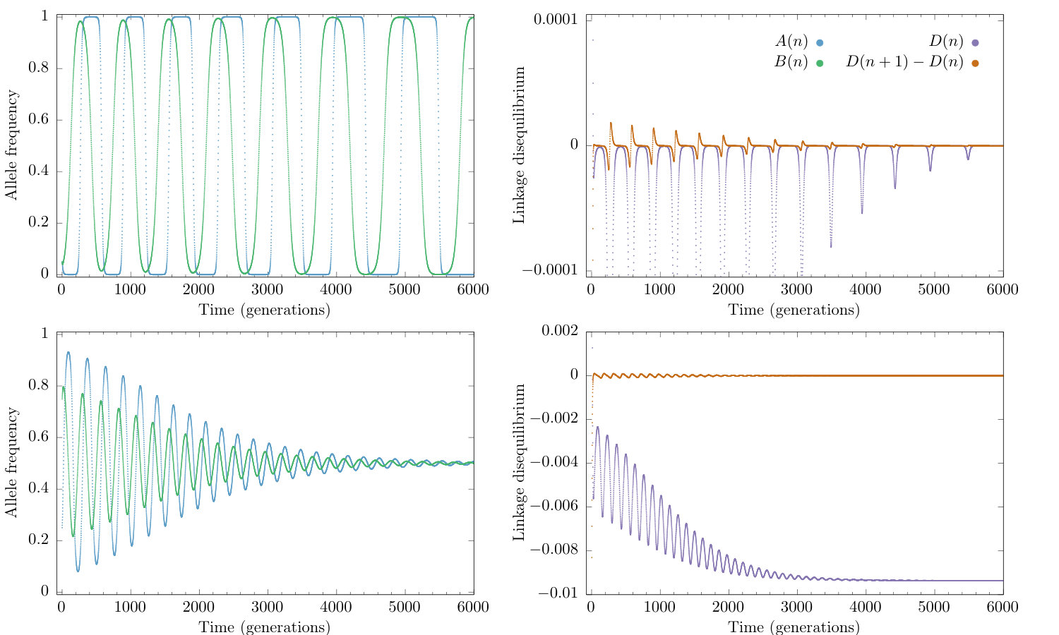 Figure 1
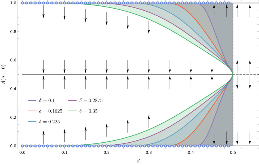 Figure 2
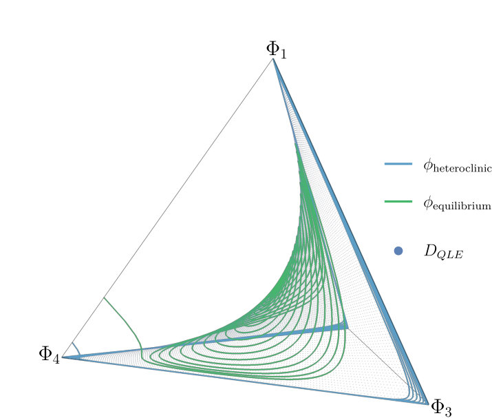 Figure 3
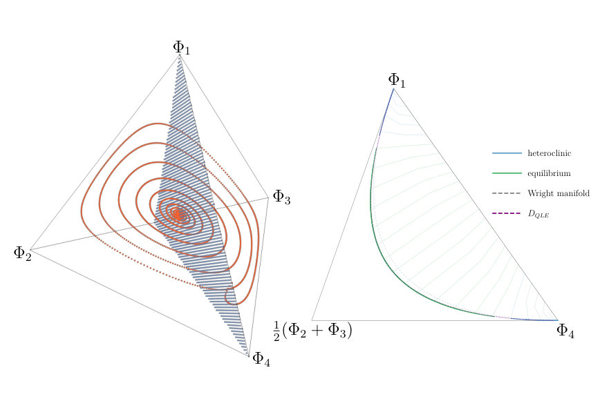 Figure 4
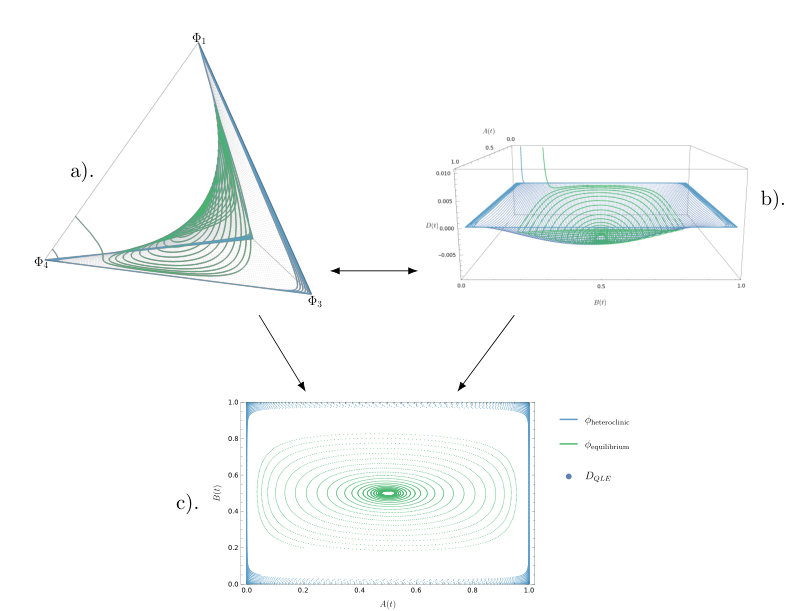 Figure 5
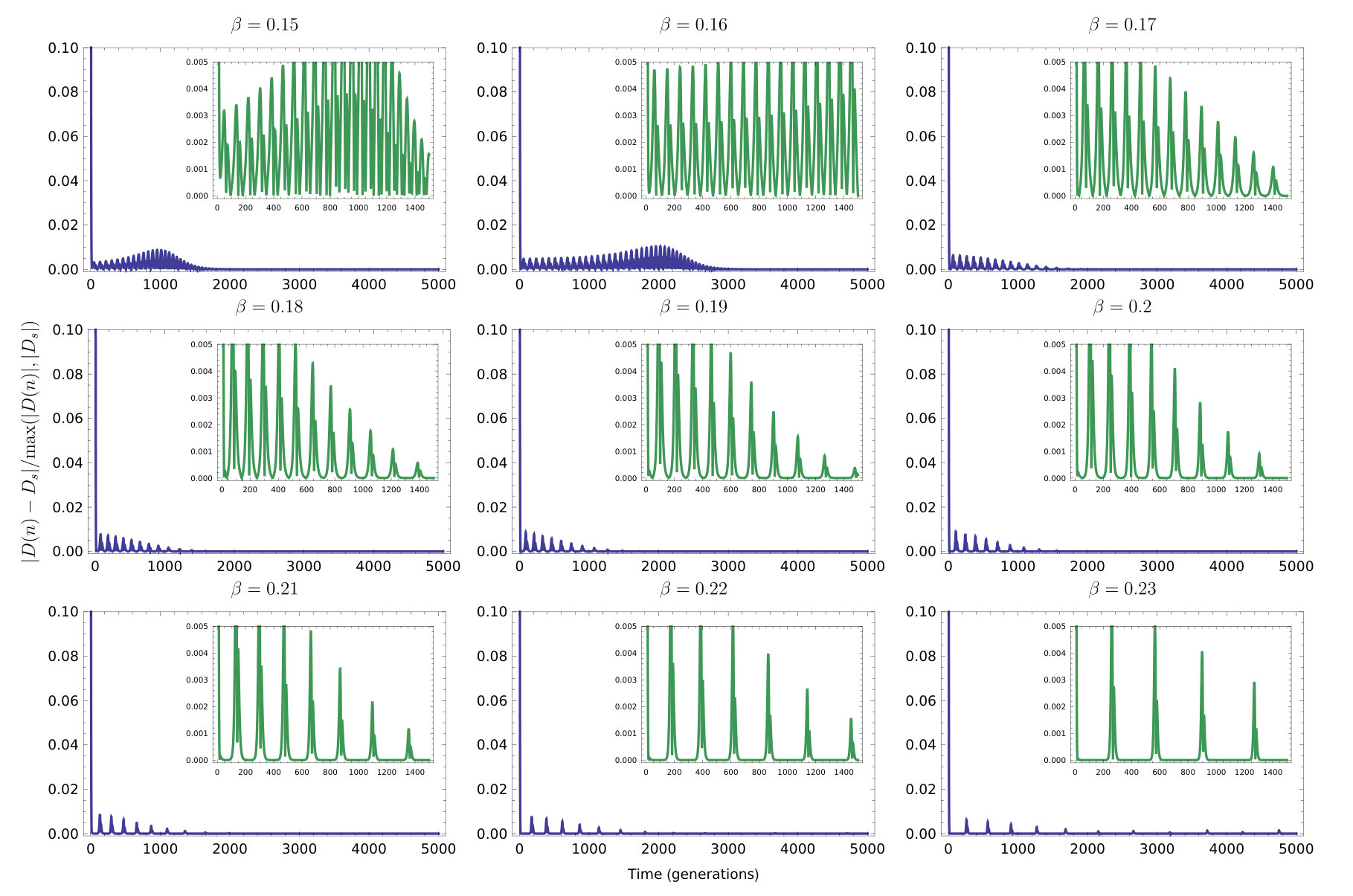 Figure 6
| Eigenvalue | ||||
|---|---|---|---|---|
| Type | ||||
| Equilibria | & | & | ||
| Eigenvalue | ||||
|---|---|---|---|---|
| Type | ||||
| Condition | ||||
| Eigenvalue | ||||
|---|---|---|---|---|
| Type | ||||
| Condition | ||||
Peer Reviews
No public reviews on file for this paper yet. If you reviewed it on a platform where reviews are public (OpenReview, ICLR, NeurIPS, ICML), you can paste yours below so the community can read it here.
Videos
No videos yet. Explain this paper in a talk, walkthrough, or lecture? Add one.
Taxonomy
TopicsEvolution and Genetic Dynamics · Gene Regulatory Network Analysis · Mathematical and Theoretical Epidemiology and Ecology Models
Stable cycling in quasi-linkage equilibrium: fluctuating dynamics under gene
conversion and selection
Timothy W. Russell
Matthew J. Russell
Francisco Úbeda
Vincent A.A. Jansen
School of Biological Sciences, Royal Holloway University of London, Egham, Surrey, TW20 0EX, UK
School of Mathematical Sciences, University of Nottingham, University Park, Nottingham, NG7 2RD, UK
Abstract
Genetic systems with multiple loci can have complex dynamics. For example, mean fitness need not always increase and stable cycling is possible. Here, we study the dynamics of a genetic system inspired by the molecular biology of recognition-dependent double strand breaks and repair as it happens in recombination hotspots. The model shows slow-fast dynamics in which the system converges to the quasi-linkage equilibrium (QLE) manifold. On this manifold, sustained cycling is possible as the dynamics approach a heteroclinic cycle, in which allele frequencies alternate between near extinction and near fixation. We find a closed-form approximation for the QLE manifold and use it to simplify the model. For the simplified model, we can analytically calculate the stability of the heteroclinic cycle. In the discrete-time model the cycle is always stable; in a continuous-time approximation, the cycle is always unstable. This demonstrates that complex dynamics are possible under quasi-linkage equilibrium.
keywords:
Quasi-linkage equilibrium , Slow manifold , Lyapunov function , Global stability , Multiple time-scales
††journal: Journal of Theoretical Biology
1 Introduction
Genetic equilibrium, the idea that gene frequencies are the same from one generation to the next, was the focus of early work on population genetics. The attention shifted when it was discovered that one-locus viability models can exhibit cycling behaviour and genetic equilibrium does not have to be achieved (Kimura, 1958; Hadeler and Liberman, 1975; Asmussen and Feldman, 1977; Cressman, 1988). Further investigation showed that two-locus viability models with recombination can also exhibit cycling behaviour (Akin, 1979; Hastings, 1981; Akin, 1982, 1983, 1987).
The discrete-time selection-recombination equations (Lewontin and Kojima, 1960; Bürger, 2000) have provided a determinsitic model for changes in the genetic make up of a population. Despite the fact that these equations are often used to study the properties of stable equilibria, they are inherently nonlinear, meaning even the most simple formulations of the equations can have complex dynamics. Examples include limit cycles (Akin, 1983) and heteroclinic cycles (Haig and Grafen, 1991; Úbeda et al., 2019). Whether the cycles are maintained indefinitely or eventually die out (i.e. their stability properties) is mathematically challenging and of significant biological importance. This is the focus of the research we present here.
Many genetic processes within an interacting population of individuals can be captured by the selection-recombination equations, as they allow for arbitrary selection regimes defined by model-specific fitness matrices. Here, we investigate the stability of cycles in two-locus genetic systems characterised by a specific interaction between selection, gene conversion and crossover. This interaction corresponds to a model of the evolution of recombination hotspots (Úbeda et al., 2019). However, we re-write this model in standard selection-recombination equations form by noticing that the effect of conversion in Úbeda et al. (2019) can be split into its effect on selection (and incorporated to the selection component of the standard selection-recombination equation) and its effect on formation of double heterozygotes (and incorporated into the recombination component of the standard selection-recombination equation). Furthermore, while the model in Úbeda et al. (2019) assumes that the values taken by the selection-recombination parameters are constrained by their biological interdependence, here we assume that the parameter values are independent and not limited by biological constraints. In doing so, we allow for multiple forms of interaction between selection, conversion and crossover, provided they produce the same equations. This formulation allow us to focus on the mathematical properties of the generalised model.
Biologically, the processes in our model are initiated by recognition between a protein formed by a modifier gene and a target locus, whereby the protein interacts with the target, initiating conversion and potentially crossover (Úbeda and Wilkins, 2011; Úbeda et al., 2019). Other than the evolution of recombination hotspots (Úbeda and Wilkins, 2011; Úbeda et al., 2019), examples of similar recognition-initiated interactions producing sustained cycling include: the evolution of homing endonucleases (Yahara et al., 2009), the evolution of meiotic drive (Haig and Grafen, 1991), the evolution of host-parasite interactions (Sasaki et al., 2002) and the evolution of altruism via tag based recognition (Jansen and Van Baalen, 2006).
If selection is weak, stable cycling cannot occur within the two-locus selection-recombination equations if the equilibria are hyperbolic (Nagylaki et al., 1999; Pontz et al., 2018). These conditions produce dynamics which converge to a stable equilibrium. Under weak selection, the argument by Nagylaki et al. (1999) uses the existence of an invariant stable manifold which attracts the dynamics. On this attracting manifold, the dynamics are gradient-like and converge to equilibrium (Pugh et al., 1977). This manifold is known in genetics as the quasi-linkage equilibrium (QLE) manifold (Kimura, 1965). It is the set of states defined by the property that linkage disequilibrium changes an order of magnitude slower than the allele frequencies (Kimura, 1965).
In geometrical terms, this means that the dynamics approach a manifold after a short initial time. If an approximate expression for such a manifold can be found, it can be exploited mathematically to simplify the system (Constable and McKane, 2017). This is usually done by assuming that selection in the model is weak (Barton, 1995; Nagylaki et al., 1999; Kirkpatrick et al., 2002; Lion, 2018). We identify the linkage disequilibrium as a fast variable in our model, isolate it using a coordinate transformation and find an approximation of the surface to which the dynamics converge. Here we show that the existence of a time-scale separation between variables and hence attraction to the QLE manifold is not exclusively associated with simple dynamics which are characterised by gradient-like convergence to an interior equilibrium.
The model presented here has complex dynamics, such as bistability and a global bifurcation. We show that, in such a system, it is still possible to find an approximate yet accurate explicit expression for the QLE manifold. For analytical tractability, following standard methods in population genetics, we derive a continuous-time approximation to our discrete-time model (Nagylaki et al., 1999; Bürger, 2000; Pontz et al., 2018). We use this continuous-time approximation to find an expression for the QLE manifold. We go on to use this to constrain the dynamics analytically to this surface, reducing the dimension of the system. We are then able to calculate the stability of the now-planar heteroclinic cycle that exists in our model within certain parameter regimes. Constraining the dynamics is a powerful step as it allows for the use of the only known analytic heteroclinic stability condition in discrete-time for planar cycles (Hofbauer and Schlag, 2000). In the vicinity of this heteroclinic cycle, strong fluctuations are possible on the QLE manifold.
Finally, we numerically assess the accuracy of our approximation of the QLE manifold against both sources of error: the quasi steady-state assumption and the use of the continuous-time derived manifold within the discrete-time system. We find that the manifold is a good approximation for the discrete-time system for both damped oscillations towards the unique interior equilibrium and the approach towards the heteroclinic cycle.
2 The model
We investigate the dynamics of haplotype frequencies of two alleles at two interacting loci, in an infinite population, undergoing a specific selection regime (uniquely defining the fitness matrix ), recombination and random union of gametes (panmixia). Once the fitness matrix and the parameter are defined, the system of equations in question is fully defined (26). First, we describe the biological processes which justify our selection regime, then we present the resulting fitness matrix (30).
Our model describes the evolution of recombination hotspots by following the dynamics between a modifier gene — producing a recombinogenic protein — and a target gene, on which the protein binds to, causing a double-strand break and initiating recombination (Úbeda et al., 2019). This model is here re-written as a system of selection-recombination equations. This system describes the following general processes: a fitness benefit derived from recognition between modifier and target , a fitness cost derived from gene conversion and the reshuffling of alleles in double heterozygotes caused by gene conversion and crossover (Úbeda et al., 2019). Our original formulation of the model included another parameter , which we have normalised to one (without loss of generality) for simplicity.
The dynamics of the matching process between homozygotes and gene conversion leads to the following system of equations describing the frequency of each haplotype in the next generation
[TABLE]
where the linkage disequilibrium between alleles is
[TABLE]
and the population mean fitness is
[TABLE]
Superscript primes indicate the value of the variable in the next generation. The population mean fitness, , ensures that the sum of the haplotype frequencies remains constant in time. To ensure the right hand side of the difference equations does not become negative, which would imply that the number of gametes produced is negative, we require that the parameters , can only take values between 0 and 1. This can be justified by the fact parameters represent probabilities in the context of the selection-recombination equations. The parameter can only take values between 0 and .
Our fitness matrix and therefore our model has similarities with that of (Karlin et al., 1970). They study symmetric viability, meaning they impose a symmetric fitness matrix. Ours is perhaps superficially similar but has a crucial difference; our matrix is not symmetric. Our matrix results in certain local symmetries within the resulting equations — symmetries which are a hallmark of heteroclinic cycles. In that sense, our model is closer to the ones of Haig and Grafen (1991) who also studied a process with a non-symmetric fitness matrix also finding a heteroclinic cycle. We choose a specific example to study for mathematical tractability and to link it to specific biological examples.
3 Analysis and Results
The model has two different qualitative behaviours: convergence to equilibrium and sustained oscillations. In both cases, the rate-of-change of tends towards zero on a faster time scale than the rate-of-change of the allele frequencies (see Figure 1). This suggests that the system has two separate time scales and that the dynamics converge towards the QLE manifold. We will find an approximate expression for this manifold.
For brevity, we introduce and to denote the frequency of the first recombinogenic protein and its matching target allele, respectively. The frequency of the second recombinogenic protein and its target allele can then be written as and .
subsectionChange of variables
The first step towards finding an approximation of the QLE manifold is changing coordinates so that they describe the allele frequencies and linkage disequilibrium. We achieve this by transforming variables from haplotype frequencies to allele frequencies using
[TABLE]
where and take values on the interval . represents linkage disequilibrium between alleles and takes values on . If we consider (4) to be the forward transformation, we arrive at the backward transformation
[TABLE]
Transforming using (4), the discrete-time model becomes
[TABLE]
Additionally, is transformed into
[TABLE]
As these coordinates include linkage disequilibrium () explicitly, they allow for a simple interpretation of the surface of total linkage equilibrium: the Wright manifold. This surface can now be written as the part of state space where (Rice, 2004).
3.1 Equilibria and local stability
The system has a maximum of ten solutions when solving for potential equilibria. Five of these live within the positive state space of the model and are therefore biologically feasible. Four of the five biologically realistic equilibria are located at the four vertices of the tetrahedron that forms the 3-simplex (in haplotype coordinates). These corner equilibria, in allelic coordinates , are
[TABLE]
We analysed the linear stability of these equilibria in Úbeda et al. (2019) and we summarise the main results here. For our choice of parameters the equilibria and are always unstable. Moreover, if these equilibria are saddles. The equilibria and are stable if and are saddles, and thus unstable, if . Note that if or take values of either 0 or 1 then . Upon inspection of the transformed models, we find that the lines connecting the equilibria to , to , to and to are all invariant. When all these equilibria are saddles (i.e. when ) a heteroclinic connection exists:
[TABLE]
The fifth equilibrium is positioned in the interior of the simplex. For this interior equilibrium it is easily verified that and for . The interior equilibrium, in allelic coordinates, is
[TABLE]
where is the negative root of
[TABLE]
given by
[TABLE]
The positive root is larger than for and therefore the corresponding equilibrium has negative haplotype frequencies.
The multipliers of the discrete-time model (6) at the interior equilibrium are given by
[TABLE]
where denotes the value of evaluated at the interior equilibrium (Úbeda et al., 2019). The eigenvalues of the interior equilibrium of the continuous-time approximation are given by .
If then and . Therefore, in this region of parameter space, it is relatively easy to see that the interior equilibrium is a saddle (both in the discrete and the continuous-time models). Specifically, and are always negative, and for , . is always positive. If then . Eigenvalues and can now form a conjugate pair of complex eigenvalues. For the equilibrium to be locally stable in the discrete-time model we require . This leads to the conditions for local stability
[TABLE]
If this condition is always fulfilled (Úbeda et al., 2019). This stability condition (13) applies only to the discrete-time model as its continuous-time approximation (15) is always locally stable (for ).
3.2 Global stability: A Lyapunov function and heteroclinic cycle
3.2.1 A continuous-time approximate model
These results on asymptotic local stability leave the question of what the global dynamics are and, in particular, if the heteroclinic connection is an attractor, or whether orbits move away from it. While the focus of this paper is to analyse the global stability properties of the discrete-time model (1), we introduce the following continuous-time approximation of the discrete-time model (Nagylaki et al., 1999; Bürger, 2000) to aid us in this matter significantly
[TABLE]
where derivatives with respect to time are denoted by a dot above a variable. The expressions for and are given by (2) and (3), the same as in the discrete-time model. The continuous-time model written in the transformed variables is
[TABLE]
It is easy to show that the equilibria for the discrete-time model and its continuous-time approximation are the same (Bürger, 2000). Similarly, it is easy to show that the eigenvalues of the Jacobian at each equilibrium in the continuous-time model equal the discrete-time eigenvalues minus unity — a consequence of the fixed time-step in the discrete-time system. We use the continuous-time model in two ways: introducing a Lyapunov function for the interior equilibrium, showing it to be globally stable; using it to find an analytically tractable version of the approximate QLE manifold, as the expression is significantly simpler when derived from the continuous-time model.
3.2.2 Lyapunov function
For the continuous-time model it is relatively easy to show that the heteroclinic cycle repels orbits using a Lyapunov function. Before we show this, we first observe that for any solution of (15) as long as at some point in time, onwards if , and with equality only if the solution lives on the heteroclinic connection. This can easily be seen by inspecting the right hand side of the differential equation describing the change in when , which is negative everywhere on the Wright manifold, apart from on the heteroclinic connection, where it is zero. Therefore, if , then for all . This means that trajectories can pass through the Wright manifold where in only one direction, and are then confined to the region where once they have done so.
With this established, we now consider the function
[TABLE]
This function (16) serves as a natural candidate for a Lyapunov function of system (14) as it retains invariance of the system along the boundaries (where either , , or ). Indeed, for this function takes the value along the heteroclinic connection, and takes positive values anywhere else in or on the simplex. The continuous-time model with set to zero (15) is equivalent to the replicator equations for games and our Lyapunov function (16) is equivalent to that of this system, serving as its constant of motion (Hofbauer and Sigmund, 1998).
The candidate function is a Lyapunov function if for orbits which at some point pass through the Wright manifold. To show this, we inspect its time derivative along solutions of (15):
[TABLE]
The right hand side of (17) is always less than or equal to zero if , meaning is a Lyapunov function within this region. For orbits starting in the forward invariant part of state space where the value of will thus increase or stay constant over time. The -limit of these orbits must therefore be invariant sets for which either or . If the only invariant part of the Wright manifold is the heteroclinic connection, where . As the value of cannot decrease and is positive for all points in or on the simplex that are not part of the heteroclinic connection, the heteroclinic connection cannot be an -limit of these orbits, within which the only other candidates are the invariant sets contained with , which is the interior equilibrium . Any orbits starting within the parts of the simplex where will therefore move towards the interior equilibrium.
A corollary of this observation is that arbitrarily close to the heteroclinic connection, where , there will be points that are within the region of the simplex where . The Lyapunov function (16) shows that orbits starting at these points will move away from the heteroclinic connection, towards the interior equilibrium. The heteroclinic connection is therefore not stable. The interior equilibrium clearly is stable and must be the attractor for all initial points in the interior of the simplex for which initially . This shows that in the continuous-time model the heteroclinic cycle is unstable. Simulations suggest that the interior equilibrium is a global attractor within the simplex.
3.2.3 Discrete-time heteroclinic cycle
The Lyapunov argument does not carry over to the discrete-time model. In the discrete-time model, does the heteroclinic connection attract or repel? We analytically investigate this using the approximate QLE manifold in section 3.5. We also numerically investigate the regions of initial condition space in which the cycle is attracting, and the results are plotted in Figure 2. In the diagram we can distinguish two regions in parameter space with qualitatively different behaviour, and the boundary between them:
Within the first region, , the interior equilibrium is stable and attracts nearby orbits. Within this region the heteroclinic connection also attracts. Between the two attractors we find the boundary of the basins of attraction. The basin boundary moves towards the heteroclinic connection for small . 2. 2.
Within the second region . All trajectories converge to one of the corner equilibria, or , apart from orbits starting exactly at the unstable interior equilibrium 3. 3.
Between these two regions , all trajectories converge to the Wright manifold. On the Wright manifold there is a line of unstable equilibria for which , . Orbits starting on the Wright manifold with converge to the line , , and those starting with converge to the line ,
These results show that the heteroclinic connection in the discrete-time model can be stable. To find out how general this is we will next analytically determine the stability of the heteroclinic connection in the discrete-time model. First, we approximate the QLE manifold towards which the trajectories converge.
3.3 The QLE manifold
If the interior equilibrium is degenerate: in the discrete-time model the equilibrium has two real multipliers at unity (whilst the interior equilibrium of the continuous-time model has two eigenvalues at zero). Because there are two eigenvalues at unity (zero), the equilibrium will have a two dimensional center manifold. If the center manifold is the Wright manifold, the part of state space where , and where the gamete frequencies are in linkage equilibrium. The third eigenvalue has a modulus smaller than one (smaller than zero for the continuous-time model) and the associated stable manifold is given by the line . Orbits on this stable manifold move towards the center manifold.
If these two multipliers become a complex pair with real part smaller than one (or negative real part for the continuous-time model). The equilibrium within this region is hyperbolic (for all ) for the ODE (15). The same is true for the map (6) when there is not equality in the stability condition (13). The center manifold morphs into a two dimensional invariant manifold that is different from the Wright manifold and contains the interior equilibrium (9). On this manifold, orbits cycle around the equilibrium. The invariant manifold containing the third eigenvector, the line on which , remains in existence. Over this line, orbits quickly converge towards the equilibrium and as they approach the linkage disequilibrium, changes rapidly while the allele frequencies and remain unchanged. Other orbits show a similar behaviour (see Figure 3): orbits generally converge towards the two dimensional manifold. Once orbits are close to this manifold the orbits move slowly towards either the interior equilibrium or the heteroclinic cycle, depending on the initial conditions (see Figure 2).
To approximate the QLE manifold, we will use a quasi-steady state argument. Specifically, we say that the change in linkage disequilibrium occurs on a much faster time scale than changes in the allele frequencies and will therefore settle on a quasi-equilibrium. This means that we can assume that the allele frequencies and are effectively constant, as settles. With this assumption, we then solve the equilibrium equation for as a function of the allele frequencies, . It turns out that this gives a good approximation for the QLE manifold for the discrete-time model as well as the continuous-time approximation.
Simulations suggest that the gamete frequencies are attracted towards the manifold where they are in quasi-linkage equilibrium. We approximate the QLE manifold by
[TABLE]
As we show in B the relevant slow time-scale is proportional to .
3.4 Simplification by reducing to allele frequencies
Given the tendency of the haplotype frequencies to settle on the QLE, one would expect that if , the dynamics proceed to the QLE manifold, and that the allele frequencies then change slowly, either towards, or away from the interior equilibrium. This is indeed what happens in the vicinity of the interior equilibrium. Further away from equilibrium, and in particular in the vicinity of the heteroclinic cycle, this is not necessarily true. It is possible that the manifold is situated outside the simplex in which all gamete frequencies are positive. If that is the case, the dynamics will be constrained by the edges of the simplex.
Inside the simplex, if . If the manifold, , cuts through the sides of the simplex, it can only be on the faces where , which is when or . In terms of allele frequencies , that is when or when The approximate manifold to which the dynamics are drawn is thus given by , where
[TABLE]
and we will use this to simplify the dynamics; in particular we will use it to determine the stability of the heteroclinic cycle.
The system constrained to the attracting manifold is given by just two equations, describing the frequencies of and on the slow manifold,
[TABLE]
where
[TABLE]
The dimensionality is now reduced and the system is significantly simplified. We can now study and depict our model as a two dimensional system (Figure 5). The stability of the heteroclinic cycle is governed by the magnitude of the eigenvalues in the connected saddles that make up the cycle. In the planar system this is relatively simple to do.
3.5 Stability of heteroclinic cycle in the discrete-time model
To study the stability of our heteroclinic cycle, we use the condition derived in Hofbauer and Schlag (2000) which determines whether a planar discrete-time heteroclinic cycle is attracting or not. The condition involves the product of the ratio of the logarithm of the expanding () eigenvalues and the absolute value of the logarithm of the contracting eigenvalues () at the saddle equilibria ( where ) the heteroclinic cycle travels between. We follow their notation and use to denote each individual ratio and to denote the product of the ,
[TABLE]
For our model, and therefore . We are then able to state the stability condition: a planar discrete-time heteroclinic cycle is asymptotically stable if and is unstable if (Hofbauer and Schlag, 2000). The specific eigenvalues for the equilibria and their type are given in Table 2. Their derivation can be found in C.
Calculating using the eigenvalues in Table 2, we arrive at the condition for stability of the heteroclinic cycle
[TABLE]
which, if , can be rewritten as
[TABLE]
In this form, it is readily seen that (23) is always satisfied if Therefore, in our discrete-time model constrained to the QLE manifold (20), the heteroclinic cycle is always asymptotically stable if it exists.
3.6 Justifying the use of derived from the continuous-time model
In Figure 6, we show the relative error between the value of , the linkage disequilibrium within the discrete-time model (1), and , the approximate slow manifold derived using the continuous-time approximation of the discrete-time system, finding the difference to be small. The error is computed using
[TABLE]
a modified form of the relative error between the approximate manifold , and the -component of a trajectory of the discrete-time system, which aims to avoid division by zero when one of the quantities is very small. The standard relative error expression could be problematic in this case, since the orbits are close to the manifold. We produce a time series of the distance between the -component of the discrete-time orbit and the value of evaluated at the values of the other variables along the orbit. This indicates that the continuous-time manifold, , provides a good approximation for the discrete-time dynamics.
4 Discussion
We studied a genetic system with viability selection and gene conversion that encompass a wide range of variants where selection can be derived from different aspects of the recombinational process (Úbeda and Wilkins, 2011; Úbeda et al., 2019). We show that the selection regime associated with a fitness benefit derived from a sequence recognition (), a fitness cost derived from a gene conversion () altogether with the reshuffling of alleles in double heterozygotes induced by gene conversion and crossover (), can lead to stable cycling dynamics in the two-locus, two-alleles model. Our model is most similar to that of Haig and Grafen (1991), because in both models the often assumed symmetry of the fitness matrix (Karlin et al., 1970) is broken. The fluctuations that feature in the model are caused by selection for one allele burning out a target sequence followed by selection for an alternative allele that can burn out the sequence that replaced the old one. This pattern can repeat indefinitely and the resulting dynamics form a heteroclinic cycle (Úbeda et al., 2019). To find out if sustained fluctuations are possible in either of our model variants we investigated whether the heteroclinic cycle attracts or repels (Hofbauer and Schlag, 2000).
We found that haplotype frequencies settle quickly on a state depending on the allele frequencies in the population, and the allele frequencies change on a slower time scale than the linkage disequilibrium (Kimura, 1965). After identifying the linkage disequilibrium as a good candidate for the fast variable, we performed the nonlinear change of variables from haplotype to allele frequencies, which introduces as an explicit variable. We then apply a quasi-steady state assumption to and solve the resulting algebraic equation for , which we use to reduce the dimension of our system by removing dependency on altogether (Figure 5) (Kuehn, 2015). We find that the dynamics don’t necessarily converge to a single stable interior (polymorphic) equilibrium. We thus provide a biological example of a doubly degenerate system that admits cycling.
After reducing the dimensionality, we found explicit conditions for stability of the heteroclinic cycles. Namely, the discrete-time model allows a heteroclinic cycle that is stable if ; on the other hand, its continuous-time approximation has a heteroclinic cycle that is always unstable and the dynamics eventually settle on an equilibrium. Furthermore, we established numerically the basin of attraction for the heteroclinic cycle and studied the accuracy of the closed-form approximation of the QLE manifold used to constrain the dynamics (Figure 6).
The equilibria of the discrete and continuous-time models are the same (Bürger, 2000). However, the stability of the heteroclinic cycle differs between the two models: the discrete-time model can have an attracting heteroclinic cycle and a stable equilibrium, and thus has a region of bistability in parameter space; however, its continuous-time approximation has, in the same region of parameter space, , a globally attracting interior equilibrium point. From a dynamical systems point of view this is not a surprise: it is well known that similar nonlinear discrete and continuous-time models can differ in various ways (May, 1976).
However, preliminary results show that if the population in the model is finite and multinomial sampling is used to pick the individuals who mate and are replaced (Wright, 1969; Úbeda et al., 2019) — producing a stochastic and more biologically realistic version of our model — we see the gap between the discrete-time model and continuous-time approximation bridged. Indeed, similar oscillatory behaviour is now observed in both models. In fact, we see the two models behaving almost identically when the population is finite, just differing in time scale. We also observe that the deterministic slow manifold, , is a good approximation for the dynamics of the stochastic model, as shown to be possible in some systems by (Constable and McKane, 2017). An in depth analysis of the stochastic model however, is beyond the scope of this paper. Further work could use to simplify the dynamics of the stochastic implementation of the model. Globally attracting invariant QLE manifolds have recently been found to exist under certain parameter regimes in the continuous-time two locus-two allele selection-recombination equations by Baigent and Seymenoglu (2018).
Similar analyses using quasi-equilibria involving variables other than linkage disequilibrium have been conducted (Van Baalen and Rand, 1998; Day et al., 2011; Lion and Gandon, 2016; Lion, 2018). These models are evolutionary-ecological rather than population genetic models, and rely on the weak selection approximation, but they still observe a rapid convergence to quasi-linkage equilibrium. Our approach to studying the QLE manifold is very general, applicable to any system showing a significant separation of time-scales. Any genetic system of this sort converges to quasi-linkage equilibrium and therefore under an appropriate transformation of variables — one which isolates the fast subsystem — can be analysed in a similar fashion. Therefore, treating the QLE manifold as an slow manifold and using linkage disequilibrium as a coordinate to approximate this surface explicitly, is a powerful technique for other genetic systems and even evolutionary ecological models.
Multi-locus models can have complex dynamics (Hastings, 1981; Hofbauer and Iooss, 1984; Haig and Grafen, 1991; Úbeda et al., 2019). It appears that most analyses of multi-locus models have been carried out under weak selection assumptions, in which case the dynamics are relatively simple: stable cycling is generally not possible and the dynamics go to an equilibrium (Nagylaki et al., 1999). The weak selection assumption allows for general analytic results (Akin, 1982; Hofbauer, 1985; Barton, 1995; Nagylaki et al., 1999; Kirkpatrick et al., 2002), often invoking the use of the QLE. Under weak selection, stable cycling and complex dynamics do not occur if the equilibria are not degenerate and therefore complex dynamics are not observed under QLE. This association of QLE with weak selection and stability might have led to the impression that complex dynamics are not compatible with quasi-linkage equilibrium (Pomiankowski and Bridle, 2004). What we have shown here is that complex dynamics are possible and, furthermore, are played out in a state of quasi-linkage equilibrium showing the association between QLE and convergence to equilibrium to not be true in general: it is possible to find continued fluctuations and sudden changes in the genetic make up in a population at quasi-linkage equilibrium.
Appendix A Deriving the discrete-time model
Our model (Úbeda et al., 2019) can be written as a particular case of the model known as the selection-recombination equations presented in (Lewontin and Kojima, 1960; Nagylaki et al., 1999; Bürger, 2000; Ubeda and Haig, 2005) and many other papers (Nagylaki et al., 1999). In the general model, haplotype frequencies evolve according to
[TABLE]
where denotes the frequency of haplotype , is the number of alleles and represents the discrete time step. The recombination terms have different signs depending on the haplotype, provided by for haplotype . Specifically, for a two-locus two-allele implementation of the model, is defined as
[TABLE]
The marginal mean fitness of a haplotype whose frequency is is given by
[TABLE]
and the mean fitness of the population is given by
[TABLE]
Due to the normalisation of the right hand side of the governing equations of the model by the mean fitness of the population, the sum of the haplotype frequencies is always one. This means the state space of the model is the simplex of dimension , where is the number of alleles and is the number of loci.
Fitnesses for the two-locus two-allele version of our model are derived by computing all of the frequencies of offspring given by each possible mating combination. Due to the symmetries on the allele types determining when recombination occurs, the linkage disequilibrium is the same for each haplotype and therefore can be taken out of the fitness matrix. This is clearly true in the more general versions of the model, meaning the linkage terms are separate in the statement of the general model equations (26). After this, and other simplifications which are possible due to symmetries in the gene conversion process and the viability benefits derived from crossover, we arrive at the following fitness matrix for the two allele two loci version of the model
[TABLE]
Applying our specific fitness matrix to the general model given gives the following system of equations
[TABLE]
Expanding the brackets in system (31) and applying the conservation law for the total population, , we can simply the system to
[TABLE]
where and and the population mean fitness is
[TABLE]
Appendix B Isolation of the multiple time-scales
The region of parameter space for which the following arguments hold is where the heteroclinic cycle exists and is attracting in the discrete-time model, i.e. .
B.1 Time-scale separation nearby the interior equilibrium
We find three distinct time-scales in the dynamics of the linearised system nearby the interior equilibrium. Recall that the eigenvalues of the interior equilibrium of the continuous-time model are given by
[TABLE]
where If then The interior equilibrium in that case is a saddle. If then . Eigenvalues and then are complex with negative real parts and the interior equilibrium is always locally stable.
We introduce the parameter
[TABLE]
which is small near the boundary of the region of parameter space in which we observe time-scale separation, . We substitute this definition into the equations and compute the eigenvalues at the interior equilibrium (9). For , the eigenvalues satisfy the identities
[TABLE]
The dynamics of the system linearised around the interior equilibrium (9) operate on three distinct time-scales: , and . If the time scales separate as The second and third time-scales are associated with the motion within the QLE manifold, while the first relates to the approach towards the QLE manifold. Under this condition, the approach is very fast compared to the dynamics on the manifold, which justifies making a quasi-steady state assumption. This behaviour can be observed in Figure 3 where the approach to QLE is very fast with associated time-scale , and much faster than the cyclic behaviour on the manifold, which acts on time-scale , which in turn is faster than the approach to equilibrium which acts on time-scale .
Note that the separation of time-scales is a direct consequence of the double degeneracy of the interior equilibrium (9). Specifically, when , and hence , two eigenvalues are zero. If the third eigenvalue is much smaller than zero, for small and continuous dependence of the eigenvalues on , the separation of time scales follows. This implies that the existence of a two-dimensional slow manifold is a generic result in the proximity of a double degeneracy and independent of the details of the model.
B.2 Time-scale separation in the full system
We introduce the new variables
[TABLE]
If , these definitions implicitly define and locally as functions of and and therefore the inverse transformation exists.
Rewriting the continuous-time model (15) in the new variables (37),
[TABLE]
Using (35), this can be written as
[TABLE]
When is small, the form of (39) isolates three distinct time-scales. The variable is changing at the fastest time-scale, and for small the variables and (and and ) are effectively constant. If and are constant, the variable has an equilibrium at
[TABLE]
The linearised dynamics around are given by
[TABLE]
which always converges to the equilibrium . Based on this we choose . If is situated outside the simplex this argument is not relevant but a similar argument can be applied for attraction to the state
Appendix C Determining the eigenvalues of the corner equilibria
In the vicinity of the origin (), we find by Taylor expanding to second order that the QLE manifold is approximately defined by . The attracting manifold in the vicinity of the origin is approximately
[TABLE]
We then find for the eigenvalues
Likewise, in the vicinity of the equilibrium and the QLE manifold is approximately
[TABLE]
and hence
[TABLE]
We then find for the eigenvalues
The reference list from the paper itself. Each links out to its DOI / PubMed record.
- 1Akin (1979) Akin, E., 1979. The geometry of population genetics. lect. Notes Biomath 31.
- 2Akin (1982) Akin, E., 1982. Cycling in simple genetic systems. Journal of Mathematical Biology 13, 305–324.
- 3Akin (1983) Akin, E., 1983. Hopf bifurcation in the two locus genetic model. volume 284. American Mathematical Soc.
- 4Akin (1987) Akin, E., 1987. Cycling in simple genetic systems: Ii. the symmetric cases, in: Dynamical Systems. Springer, pp. 139–153.
- 5Asmussen and Feldman (1977) Asmussen, M.A., Feldman, M.W., 1977. Density dependent selection 1: A stable feasible equilibrium may not be attainable. Journal of Theoretical Biology 64, 603–618.
- 6Baigent and Seymenoglu (2018) Baigent, S., Seymenoglu, B., 2018. Competitive selection-recombination dynamics: A new approach to studying the quasilinkage equilibrium manifold. URL: https://www.ucl.ac.uk/~zcahge 7/files/S Rpaper.pdf .
- 7Barton (1995) Barton, N.H., 1995. A general model for the evolution of recombination. Genetics Research 65, 123–144.
- 8Bürger (2000) Bürger, R., 2000. The mathematical theory of selection, recombination, and mutation. John Wiley & Sons.