TL;DR
This paper introduces a multiframe super-resolution algorithm for smartphones that directly reconstructs high-resolution RGB images from raw burst frames, leveraging natural hand tremor to improve resolution and noise without traditional demosaicing.
Contribution
It presents a novel super-resolution method that bypasses demosaicing, enhancing image quality from raw burst frames on mobile devices with real-time performance.
Findings
Achieves 100 ms processing time per 12MP frame on mobile hardware.
Improves resolution and noise performance in challenging conditions.
Serves as the basis for Google's Super-Res Zoom and Night Sight modes.
Abstract
Compared to DSLR cameras, smartphone cameras have smaller sensors, which limits their spatial resolution; smaller apertures, which limits their light gathering ability; and smaller pixels, which reduces their signal-to noise ratio. The use of color filter arrays (CFAs) requires demosaicing, which further degrades resolution. In this paper, we supplant the use of traditional demosaicing in single-frame and burst photography pipelines with a multiframe super-resolution algorithm that creates a complete RGB image directly from a burst of CFA raw images. We harness natural hand tremor, typical in handheld photography, to acquire a burst of raw frames with small offsets. These frames are then aligned and merged to form a single image with red, green, and blue values at every pixel site. This approach, which includes no explicit demosaicing step, serves to both increase image resolution and…
Click any figure to enlarge with its caption.
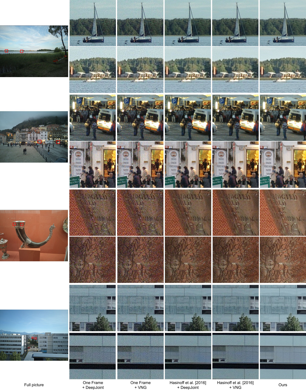 Figure 1
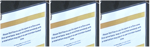 Figure 2
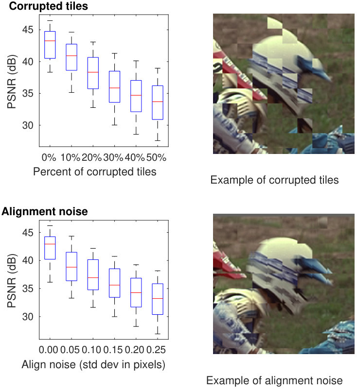 Figure 3
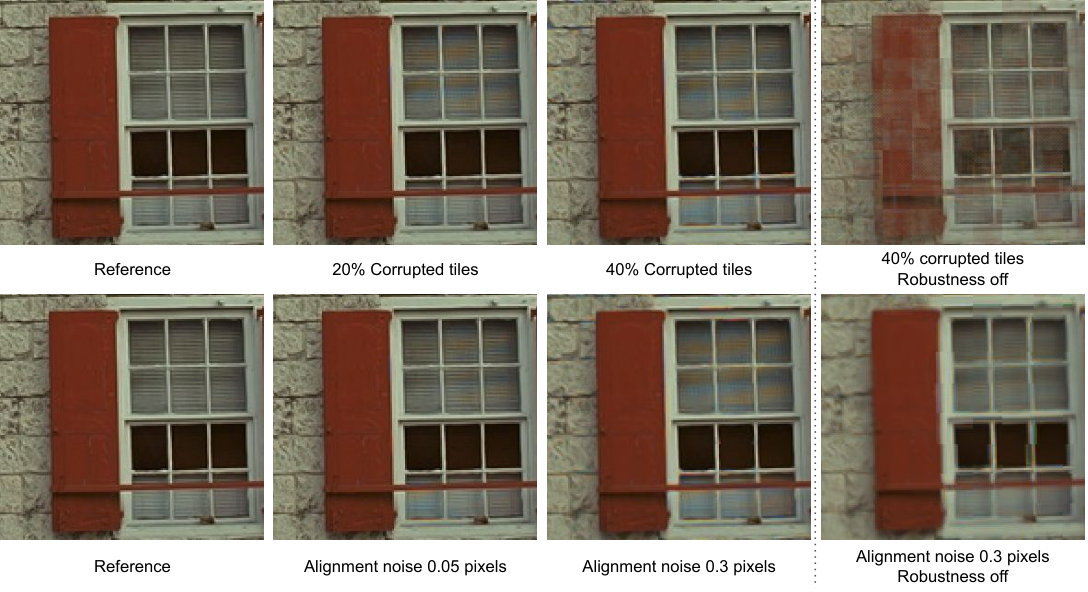 Figure 4
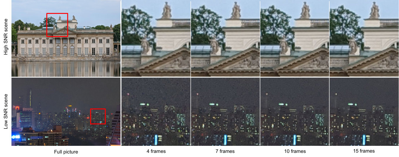 Figure 5
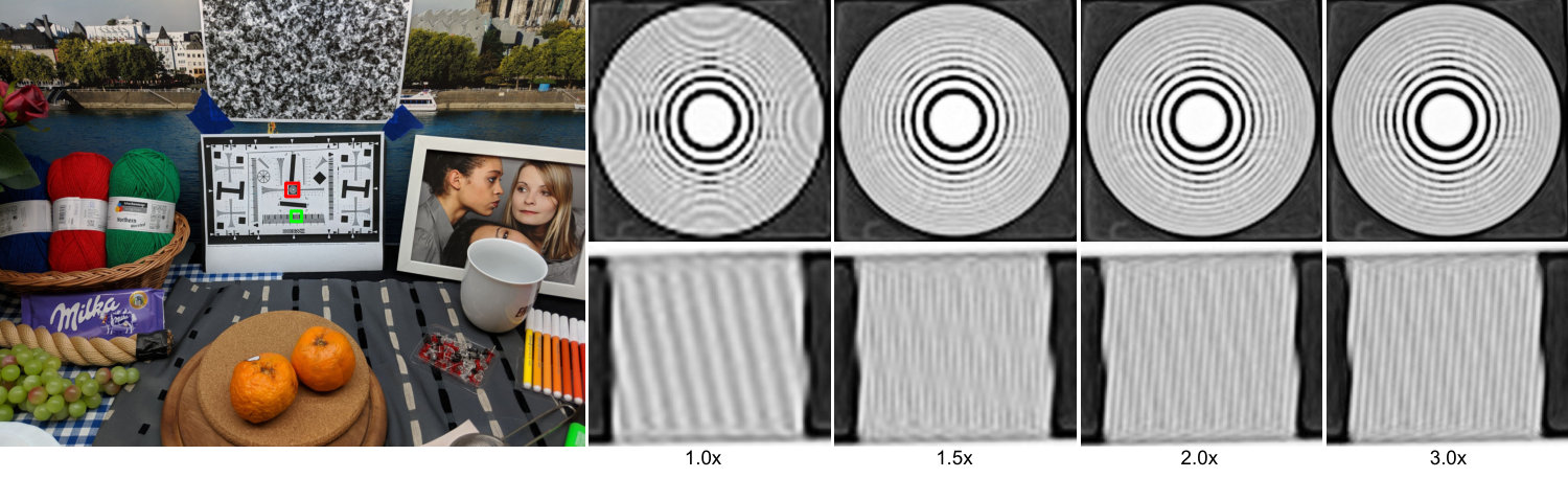 Figure 6
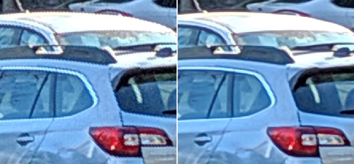 Figure 8
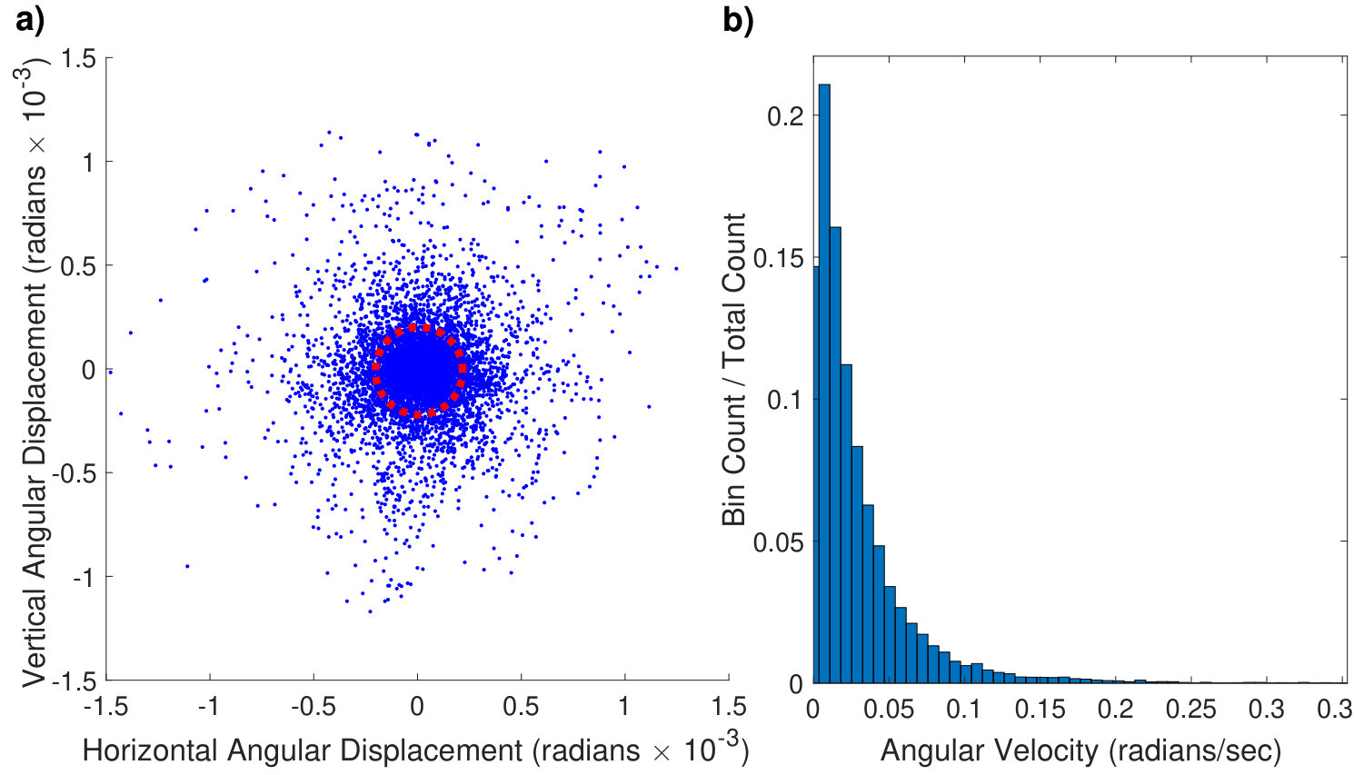 Figure 9
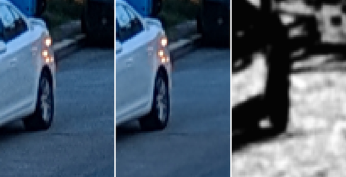 Figure 10
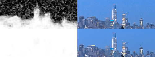 Figure 11
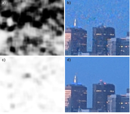 Figure 12
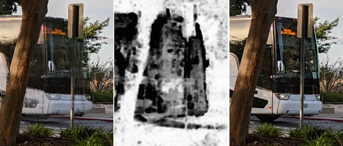 Figure 13
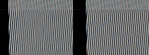 Figure 14
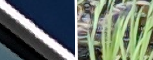 Figure 15
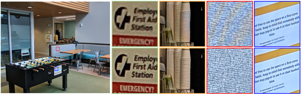 Figure 16
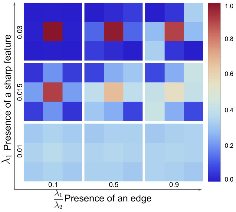 Figure 17
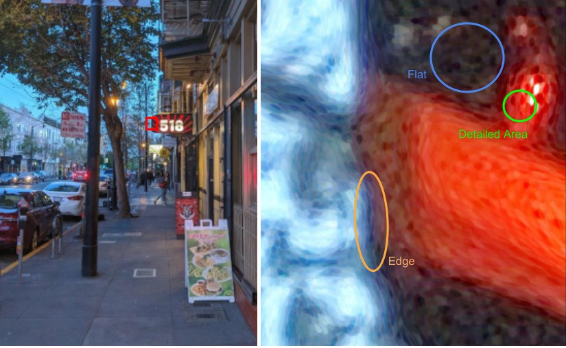 Figure 18
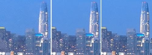 Figure 19
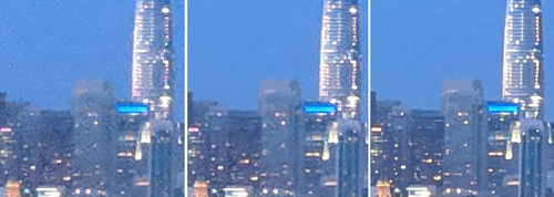 Figure 20
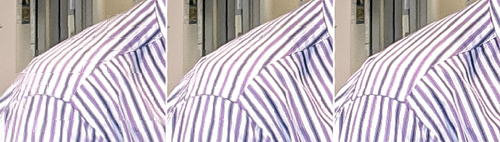 Figure 21
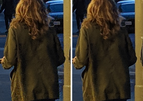 Figure 22
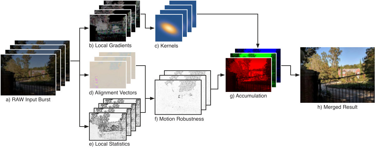 Figure 23
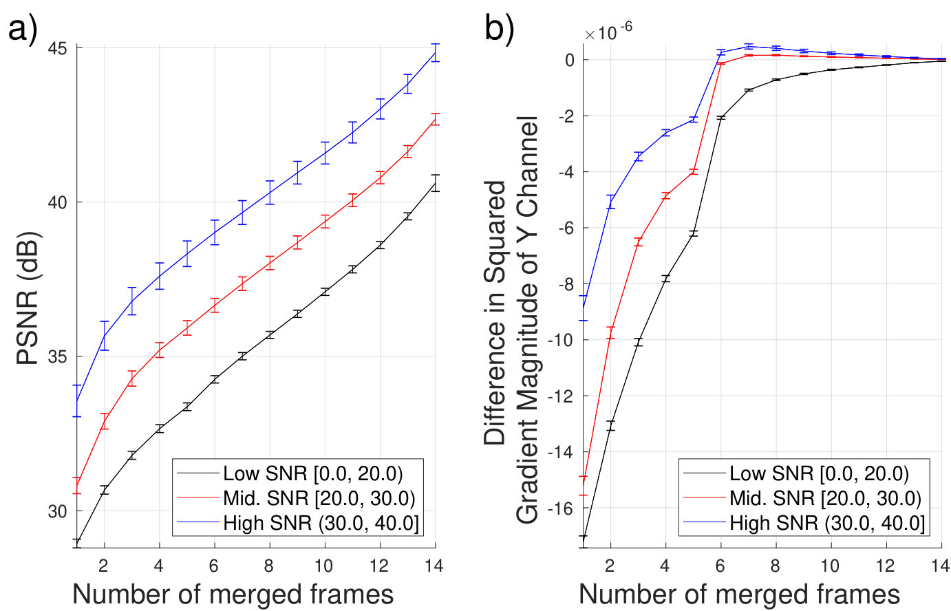 Figure 24
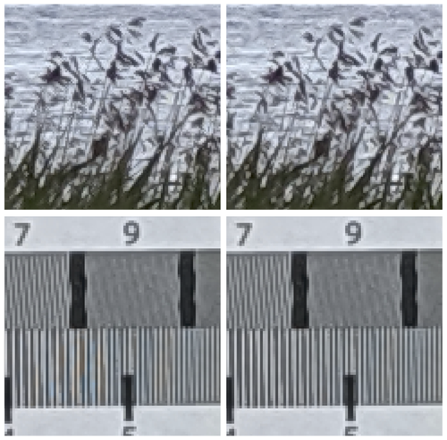 Figure 25
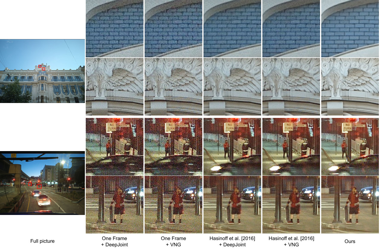 Figure 26
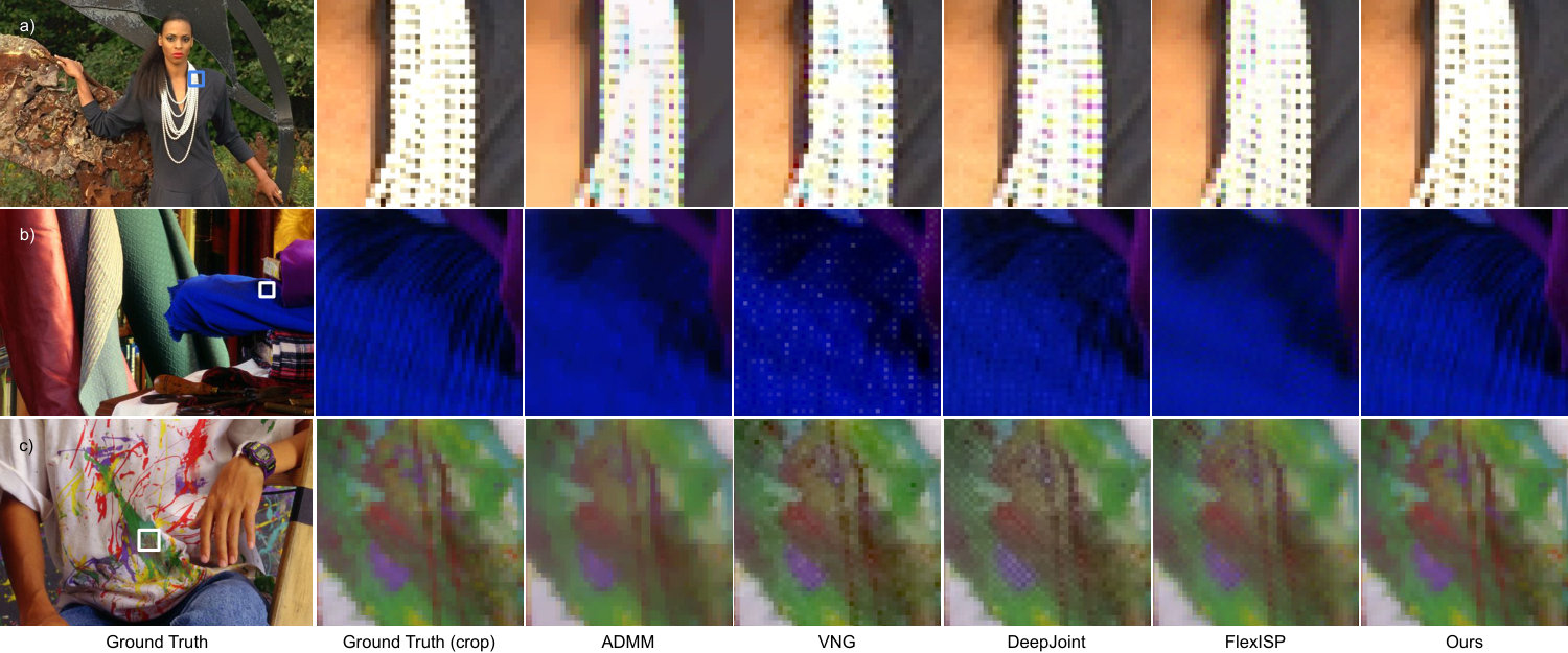 Figure 27
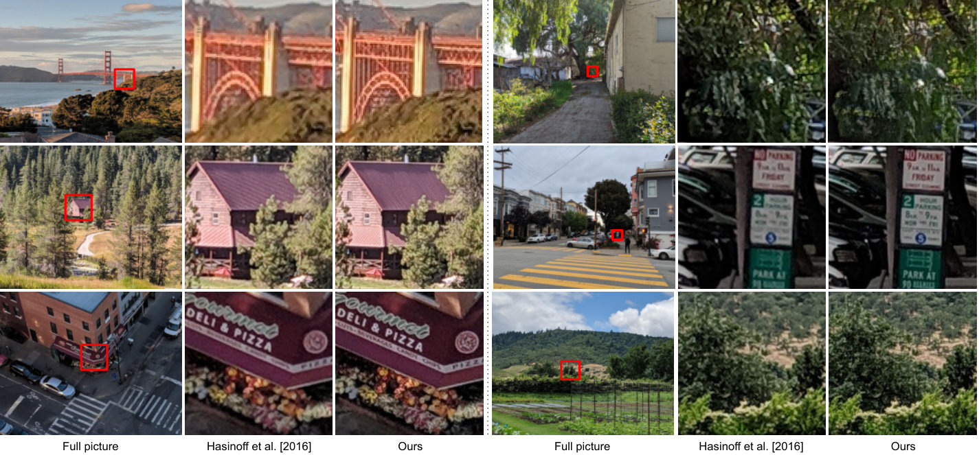 Figure 28
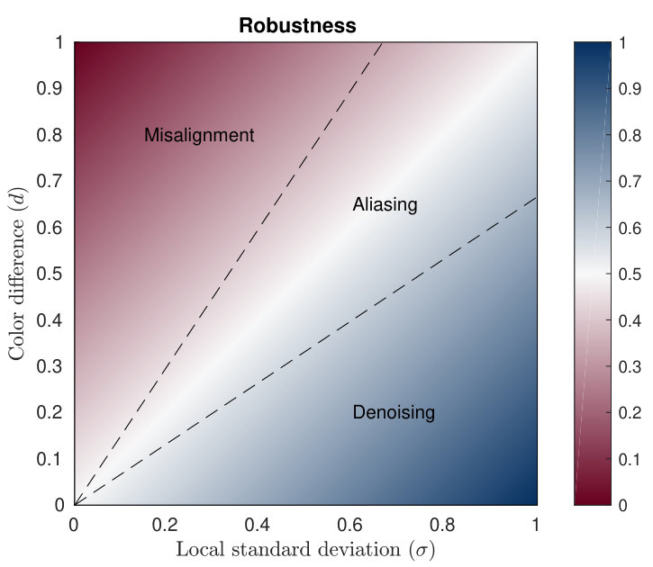 Figure 29
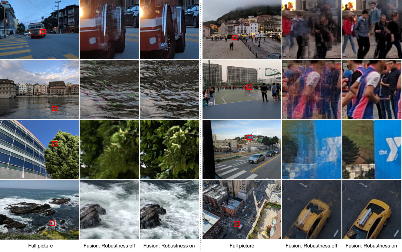 Figure 30
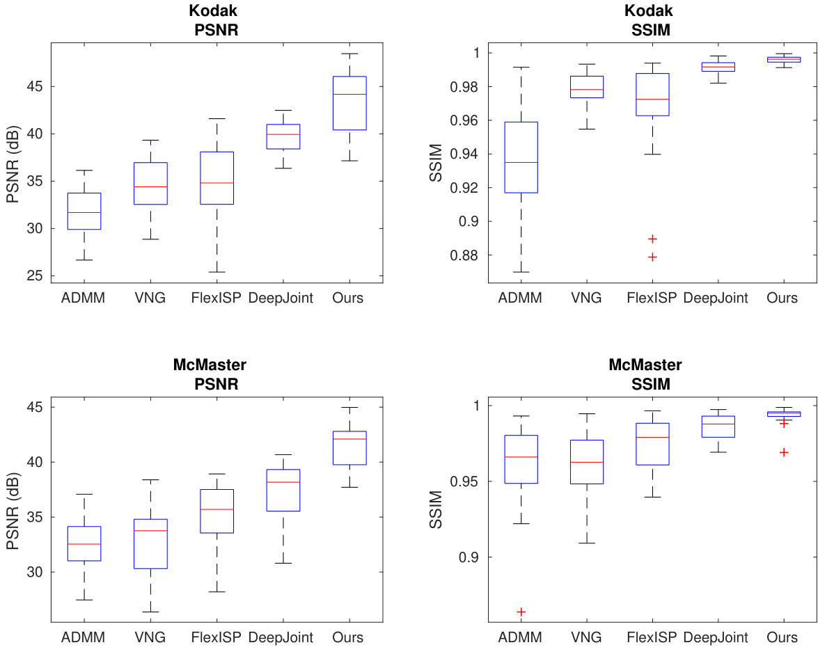 Figure 32
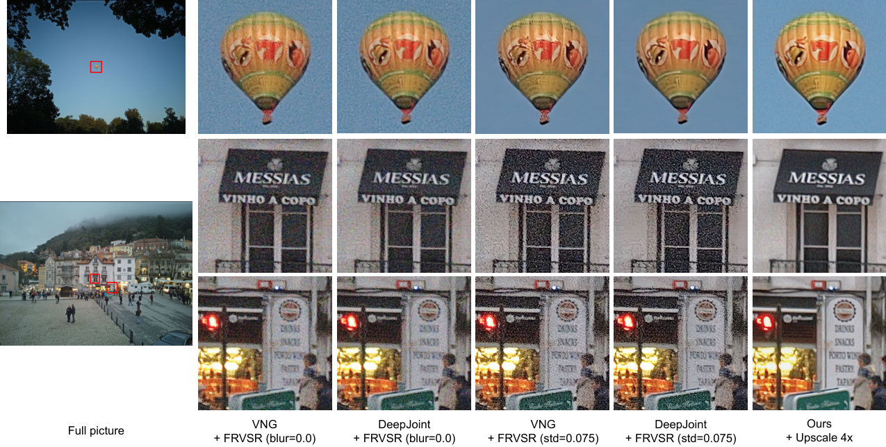 Figure 33
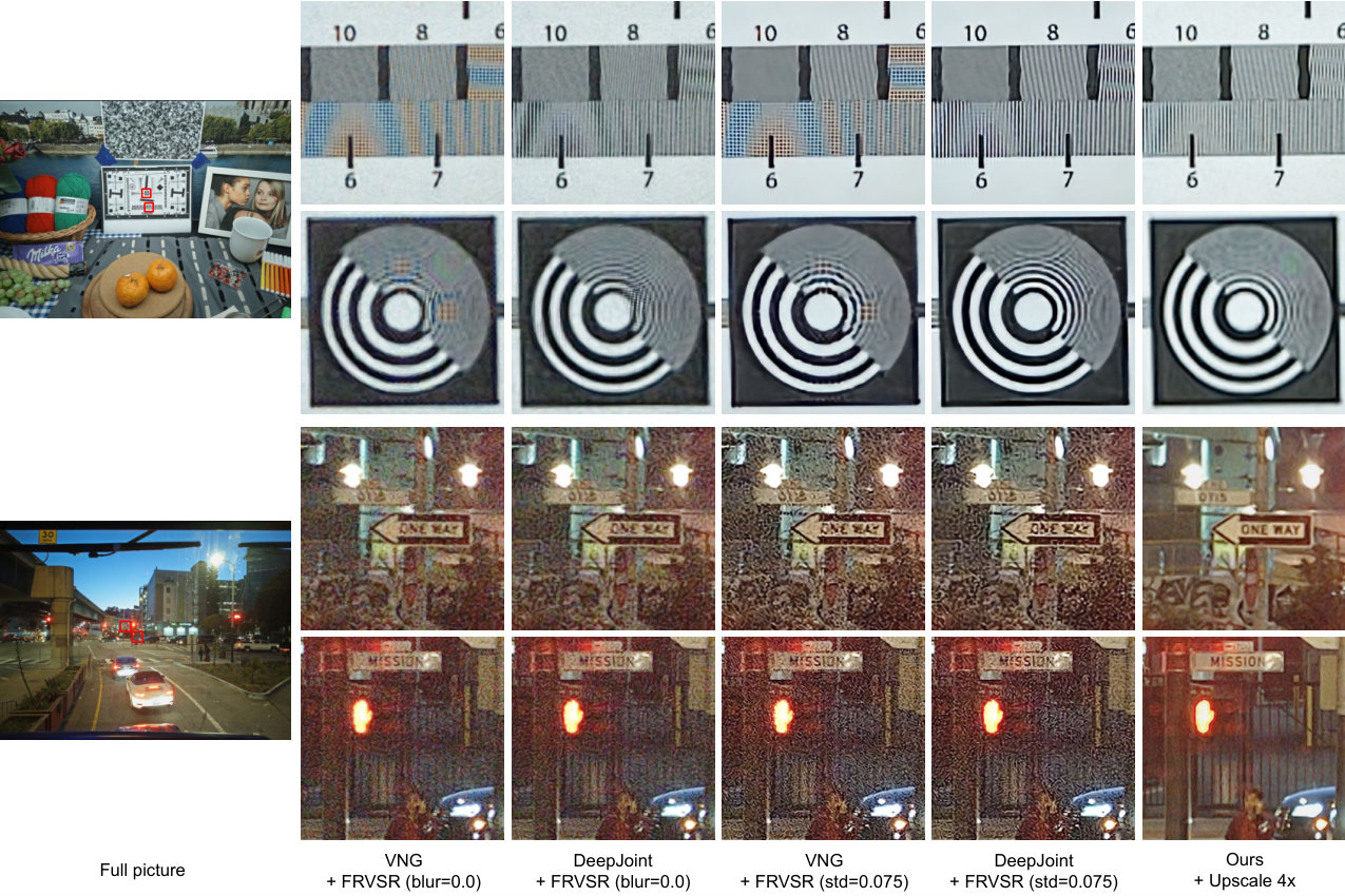 Figure 34
| Kodak | Kodak | McM | McM | MPix/s | |
|---|---|---|---|---|---|
| PSNR | SSIM | PSNR | SSIM | (higher is better) | |
| ADMM | 31.79 | 0.935 | 32.66 | 0.957 | 0.0005 (CPU) |
| VNG | 34.71 | 0.978 | 32.74 | 0.961 | 3.22 (CPU) |
| FlexISP | 35.08 | 0.967 | 35.15 | 0.975 | 3.07 (GPU) |
| DeepJoint | 39.67 | 0.991 | 37.58 | 0.986 | 0.33 (GPU) |
| Ours | 42.86 | 0.996 | 41.26 | 0.993 | 1756.9 (GPU) |
| One Frame | One Frame | Hasinoff et al. | Hasinoff et al. | ||
|---|---|---|---|---|---|
| DeepJoint | VNG | + DeepJoint | VNG | Ours | |
| One Frame + DeepJoint | - | 0.495 | 0.198 | 0.198 | 0.059 |
| One Frame + VNG | 0.505 | - | 0.099 | 0.168 | 0.059 |
| Hasinoff et al. + DeepJoint | 0.802 | 0.901 | - | 0.624 | 0.208 |
| Hasinoff et al. + VNG | 0.802 | 0.832 | 0.376 | - | 0.099 |
| Ours | 0.941 | 0.941 | 0.792 | 0.901 | - |
| GPU | Fixed cost | Cost per frame | Memory cost |
|---|---|---|---|
| Adreno 630 | 15.4 ms | 7.8 ms / MPix | 22 MB / MPix |
| GTX 980 | 0.83 ms | 0.4 ms / MPix | 22 MB / MPix |
Peer Reviews
No public reviews on file for this paper yet. If you reviewed it on a platform where reviews are public (OpenReview, ICLR, NeurIPS, ICML), you can paste yours below so the community can read it here.
Code & Models
Videos
No videos yet. Explain this paper in a talk, walkthrough, or lecture? Add one.
Handheld Multi-Frame Super-Resolution
Bartlomiej Wronski
,
Ignacio Garcia-Dorado
,
Manfred Ernst
,
Damien Kelly
,
Michael Krainin
,
Chia-Kai Liang
,
Marc Levoy
and
Peyman Milanfar
Google Research1600 Amphitheatre ParkwayMountain ViewCA94043
Abstract.
Compared to DSLR cameras, smartphone cameras have smaller sensors, which limits their spatial resolution; smaller apertures, which limits their light gathering ability; and smaller pixels, which reduces their signal-to-noise ratio. The use of color filter arrays (CFAs) requires demosaicing, which further degrades resolution. In this paper, we supplant the use of traditional demosaicing in single-frame and burst photography pipelines with a multi-frame super-resolution algorithm that creates a complete RGB image directly from a burst of CFA raw images. We harness natural hand tremor, typical in handheld photography, to acquire a burst of raw frames with small offsets. These frames are then aligned and merged to form a single image with red, green, and blue values at every pixel site. This approach, which includes no explicit demosaicing step, serves to both increase image resolution and boost signal to noise ratio. Our algorithm is robust to challenging scene conditions: local motion, occlusion, or scene changes. It runs at 100 milliseconds per 12-megapixel RAW input burst frame on mass-produced mobile phones. Specifically, the algorithm is the basis of the Super-Res Zoom feature, as well as the default merge method in Night Sight mode (whether zooming or not) on Google’s flagship phone.
computational photography, super-resolution, image processing, photography
††submissionid: 411††price: 15.00††copyright: rightsretained††journal: TOG††journalyear: 2019††journalvolume: 38††journalnumber: 4††article: 28††publicationmonth: 7††doi: 10.1145/3306346.3323024††ccs: Computing methodologies Computational photography††ccs: Computing methodologies Image processing
1. Introduction
Smartphone camera technology has advanced to the point that taking pictures with a smartphone has become the most popular form of photography [CIPA, 2018; Flickr, 2017]. Smartphone photography offers high portability and convenience, but many challenges still exist in the hardware and software design of a smartphone camera that must be overcome to enable it to compete with dedicated cameras.
Foremost among these challenges is limited spatial resolution. The resolution produced by digital image sensors is limited not only by the physical pixel count (e.g., 12-megapixel camera), but also by the presence of color filter arrays (CFA)111Also known as a color filter mosaic (CFM). like the Bayer CFA [Bayer, 1976]. Given that human vision is more sensitive to green, a quad of pixels in the sensor usually follows the Bayer pattern RGGB; i.e., 50% green, 25% red, and 25% blue. The final full-color image is generated from the spatially undersampled color channels through an interpolation process called demosaicing [Li et al., 2008].
Demosaicing algorithms operate on the assumption that the color of an area in a given image is relatively constant. Under this assumption, the color channels are highly correlated, and the aim of demosaicing is to reconstruct the undersampled color information while avoiding the introduction of any visual artifacts. Typical artifacts of demosaicing include false color artifacts such as chromatic aliases, zippering (abrupt or unnatural changes of intensity over consecutive pixels that look like a zipper), maze, false gradient, and Moiré patterns (Figure 1 top). Often, the challenge in effective demosaicing is trading off resolution and detail recovery against introducing visual artifacts. In some cases, the underlying assumption of cross-channel correlation is violated, resulting in reduced resolution and loss of details.
A significant advancement in smartphone camera technology in recent years has been the application of software-based computational photography techniques to overcome limitations in camera hardware design. Examples include techniques for increasing dynamic range [Hasinoff et al., 2016], improving signal-to-noise ratio through denoising [Mildenhall et al., 2018; Godard et al., 2018] and wide aperture effects to synthesize shallow depth-of-field [Wadhwa et al., 2018]. Many of these recent advancements have been achieved through the introduction of burst processing222We use the terms multi-frame and burst processing interchangeably to refer to the process of generating a single image from multiple images captured in rapid succession. where on a shutter press multiple acquired images are combined to produce a photo that is of greater quality than that of a single acquired image.
In this paper, we introduce an algorithm that uses signals captured across multiple shifted frames to produce higher resolution images (Figure 1 bottom). Although the underlying techniques can be generalized to any shifted signals, in this work we focus on applying the algorithm to the task of resolution enhancement and denoising in a smartphone image acquisition pipeline using burst processing. By using a multi-frame pipeline and combining different undersampled and shifted information present in different frames, we remove the need for an explicit demosaicing step.
To work on a smartphone camera, any such algorithm must:
- •
Work handheld from a single shutter press – without a tripod or deliberate motion of the camera by the user.
- •
Run at an interactive rate – the algorithm should produce the final enhanced resolution with low latency (within at most a few seconds).
- •
Be robust to local motion and scene changes – users might capture scenes with fast moving objects or scene changes. While the algorithm might not increase resolution in all such scenarios, it should not produce appreciable artifacts.
- •
Be robust to noisy input data – in low light the algorithm should not amplify noise, and should strive to reduce it.
With these criteria in mind, we have developed an algorithm that processes multiple successively captured raw frames in an online fashion. The algorithm tackles the tasks of demosaicing and super-resolution jointly and formulates the problem as the reconstruction and interpolation of a continuous signal from a set of sparse samples. Red, green and blue pixels are treated as separate signals on different planes and reconstructed simultaneously. This approach enables the production of highly detailed images even when there is no cross-channel correlation – as in the case of saturated single-channel colors. The algorithm requires no special capturing conditions; natural hand-motion produces offsets that are sufficiently random in the subpixel domain to apply multi-frame super-resolution. Additionally, since our super-resolution approach creates a continuous representation of the input, it allows us to directly create an image with a desired target magnification / zoom factor without the need for additional resampling. The algorithm works on a mobile device and incurs a computational cost of only 100 ms per 12-megapixel processed frame.
The main contributions of this work are:
- (1)
Replacing raw image demosaicing with a multi-frame super-resolution algorithm. 2. (2)
The introduction of an adaptive kernel interpolation / merge method from sparse samples (Section 5) that takes into account the local structure of the image, and adapts accordingly. 3. (3)
A motion robustness model (Section 5.2) that allows the algorithm to work with bursts containing local motion, disocclusions, and alignment/registration failures (Figure 12). 4. (4)
The analysis of natural hand tremor as the source of subpixel coverage sufficient for super-resolution (Section 4).
2. Background
2.1. Demosaicing
Demosaicing has been studied extensively [Li et al., 2008], and the literature presents a wide range of algorithms. Most methods interpolate the missing green pixels first (since they have double sampling density) and reconstruct the red and blue pixel values using color ratio [Lukac and Plataniotis, 2004] or color difference [Hirakawa and Parks, 2006]. Other approaches work in the frequency domain [Leung et al., 2011], residual space [Monno et al., 2015], use LAB homogeneity metrics [Hirakawa and Parks, 2005] or non local approaches [Duran and Buades, 2014]. More recent works use CNNs to solve the demosaicing problem such as the joint demosaicing and denoising technique by Gharbi et al. [2016]. Their key insight is to create a better training set by defining metrics and techniques for mining difficult patches from community photographs.
2.2. Multi-frame Super-resolution (SR)
Single-image approaches exploit strong priors or training data. They can suppress aliasing333In this work we refer to aliasing in signal processing terms – a signal with frequency content above half of the sampling rate that manifests as a lower frequency after sampling [Nyquist, 1928]. well, but are often limited in how much they can reconstruct from aliasing. In contrast to single frame techniques, the goal of multi-frame super-resolution is to increase the true (optical) resolution.
In the sampling theory literature, multi-frame super-resolution techniques date as far back as the ’50s [Yen, 1956] and the ’70s [Papoulis, 1977]. The work of Tsai [1984] started the modern concept of super-resolution by showing that it was possible to improve resolution by registering and fusing multiple aliased images. Irani and Peleg [1991], and then Elad and Feuer [1997] formulated the algorithmic side of super-resolution. The need for accurate subpixel registration, existence of aliasing, and good signal-to-noise levels were identified as the main requirements of practical super-resolution [Baker and Kanade, 2002; Robinson and Milanfar, 2004, 2006].
In the early 2000s, Farsiu et al. [2006] and Gotoh and Okutomi [2004] formulated super-resolution from arbitrary motion as an optimization problem that would be infeasible for interactive rates. Ben-Ezra et al. [2005] created a jitter camera prototype to do super-resolution using controlled subpixel detector shifts. This and other works inspired some commercial cameras (e.g., Sony A6000, Pentax FF K1, Olympus OM-D E-M1 or Panasonic Lumix DC-G9) to adopt multi-frame techniques, using controlled pixel shifting of the physical sensor. However, these approaches require the use of a tripod or a static scene. Video super-resolution approaches [Belekos et al., 2010; Liu and Sun, 2011; Sajjadi et al., 2018] counter those limitations and extend the idea of multi-frame super-resolution to video sequences.
2.3. Kernel Based Super-resolution and Interpolation
Takeda et al. [2006; 2007] formulated super-resolution as a kernel regression and reconstruction problem, which allows for faster processing. Around the same time, Müller et al. [2005] introduced a technique to model fluid-fluid interactions that can be rendered using kernel methods introduced by Blinn [1982]. Yu and Turk [2013] proposed an adaptive solution to the reconstructing of surfaces of particle-based fluids using anisotropic kernels. These kernels, like Takeda et al. ’s, are based on local gradient Principal Component Analysis (PCA), where the anisotropy of the kernels allows for simultaneous preservation of sharp features and smooth rendering of flat surfaces. Similar adaptive kernel based method were proposed for single image super-resolution by Hunt [2004] and for general upscaling and interpolation by Lee and Yoon [2010]. We adopt some of these ideas and generalize them to fit our use case.
2.4. Burst Photography and Raw Fusion
Burst fusion methods based on raw imagery are relatively uncommon in the literature, as they require knowledge of the photographic pipeline [Farsiu et al., 2006; Heide et al., 2014; Wu and Zhang, 2006; Gotoh and Okutomi, 2004]. Vandewalle et al. [2007] described an algorithm where information from multiple Bayer frames is separated into luminance and chrominance components and fused together to improve the CFA demosaicing. Most relevant to our work is Hasinoff et al. [2016] which introduced an end-to-end burst photography pipeline fusing multiple frames for increased dynamic range and signal-to-noise ratio. Our paper is a more general fusion approach that (a) dispenses with demosaicing, (b) produces increased resolution, and (c) enables merging onto an arbitrary grid, allowing for high quality digital zoom at modest factors (Section 7). Most recently, Li et al. [2018] proposed an optimization based algorithm for forming an RGB image directly from fused, unregistered raw frames.
2.5. Multi-frame Rendering
This work also draws on multi-frame and temporal super-resolution techniques widely used in real-time rendering (for example, in video games). Herzog et al. combined information from multiple rendered frames to increase resolution [2010]. Sousa et al. [2011] mentioned the first commercial use of robustly combining information from two frames in real-time in a video game, while Malan [2012] expanded its use to produce a image from four frames. Subsequent work [Sousa, 2013; Drobot, 2014; Karis, 2014] established temporal super-resolution techniques as state-of-the-art and standard in real-time rendering for various effects, including dynamic resolution rendering and temporal denoising. Salvi [2016] provided a theoretical explanation of commonly used local color neighborhood clipping techniques and proposed an alternative based on statistical analysis. While most of those ideas are used in a different context, we generalize their insights about detecting aliasing, misalignment and occlusion in our robustness model.
2.6. Natural Hand Tremor
While holding a camera (or any object), a natural, involuntary hand tremor is always present. The tremor is comprised of low amplitude and high frequency motion components that occur while holding steady limb postures [Schäfer, 1886]. The movement is highly periodic, with a frequency in the range of 8–12 Hz, and its movement is small in magnitude but random [Marshall and Walsh, 1956]. The motion also consists of a mechanical-reflex component that depends on the limb, and a second component that causes micro-contractions in the limb muscles [Riviere et al., 1998]. This behavior has been shown to not change with age [Sturman et al., 2005] but it can change due to disease [NIH, 2018]. In this paper, we show that the hand tremor of a user holding a mobile camera is sufficient to provide subpixel coverage for super-resolution.
3. Overview of Our Method
Our approach is visualized in Figure 2. First, a burst of raw (CFA Bayer) images is captured. For every captured frame, we align it locally with a single frame from the burst (called the base frame). Next, we estimate each frame’s local contributions through kernel regression (Section 5.1) and accumulate those contributions across the entire burst. The contributions are accumulated separately per color plane. We adjust kernel shapes based on the estimated signal features and weight the sample contributions based on a robustness model (Section 5.2). We perform per-channel normalization to obtain the final merged RGB image.
3.1. Frame Acquisition
Since our algorithm is designed to work within a typical burst processing pipeline, it is important that the processing does not increase the overall photo capture latency. Typically, a smartphone operates in a mode called Zero-Shutter Lag, where raw frames are being captured continuously to a ring buffer when the user opens and operates the camera application. On a shutter press, the most recent captured frames are sent to the camera processing pipeline. Our algorithm operates on an input burst (Figure 2 (a)) formed from those images. Relying on previously captured frames creates challenges for the super-resolution algorithm – the user can be freely moving the camera prior to the capture. The merge process must be able to deal with natural hand motion (Section 4) and cannot require additional movement or user actions.
3.2. Frame Registration and Alignment
Prior to combining frames, we place them into a common coordinate system by registering frames against the base frame to create a set of alignment vectors (Figure 2 (d)). Our alignment solution is a refined version of the algorithm used by Hasinoff et al. [2016]. The core alignment algorithm is coarse-to-fine, pyramid-based block matching that creates a pyramid representation of every input frame and performs a limited window search to find the most similar tile. Through the alignment process we obtain per patch/tile (with tile sizes of ) alignment vectors relative to the base frame.
Unlike Hasinoff et al. [2016], we require subpixel accurate alignment to achieve super-resolution. To address this issue we could use a different, dedicated registration algorithm designed for accurate subpixel estimation (e.g., Fleet and Jepson [1990]), or refine the block matching results. We opted for the latter due to its simplicity and computational efficency. We have explored estimating the subpixel offsets by fitting a quadratic curve to the block matching alignment error and finding its minimum [Kanade and Okutomi, 1991]; however, we found that super-resolution requires a more accurate method. Therefore, we refine the block matching alignment vectors by three iterations of Lucas-Kanade [1981] optical flow image warping. This approach reached the necessary accuracy while keeping the computational cost low.
3.3. Merge Process
After frames are aligned, the remainder of the merge process (Figure 2 (b-g)) is responsible for fusing the raw frames into a full RGB image. These steps constitute the core of our algorithm and will be described in greater detail in Section 5.
The merge algorithm works in an online fashion, sequentially computing the contributions of each processed frame to every output pixel by accumulating colors from a neighborhood. Those contributions are weighted by kernel weights (Section 5.1, Figure 2 (c)), modulated by the robustness mask (Section 5.2, Figure 2 (f)), and summed together separately for the red, green and blue color planes. At the end of the process, we divide the accumulated color contributions by the accumulated weights, obtaining three color planes.
The result of the merge process is a full RGB image, which can be defined at any desired resolution. This can be processed further by the typical camera pipeline (spatial denoising, color correction, tone-mapping, sharpening) or alternatively saved for further offline processing in a non-CFA raw format like Linear DNG [Adobe, 2012].
Before we explain the algorithm details, we analyze the key characteristics that enable the hand-held super-resolution.
4. Hand-held Super-Resolution
Multi-frame super-resolution requires two conditions to be fulfilled [Tsai and Huang, 1984]:
- (1)
Input frames need to be aliased, i.e., contain high frequencies that manifest themselves as false low frequencies after sampling. 2. (2)
The input must contain multiple aliased images, sampled at different subpixel offsets. This will manifest as different phases of false low frequencies in the input frames.
Having multiple lower resolution shifted and aliased images allows us to both remove the effects of aliasing in low frequencies as well as reconstruct the high frequencies. In a (mobile) camera pipeline, means an image sensor having distances between pixels larger than the spot size of the lens. Our algorithm assumes that the input raw frames are aliased (see discussion in Section 7).
Most existing multi-frame super-resolution approaches impose restrictions on the types of motion noted in . This includes commercially available products like DSLR cameras using sensor shifts of a camera placed on a tripod. Those requirements are impractical for casual photography and violate our algorithm goals; therefore we make use of natural hand motion. Some publications like Li et al. [2018] use unregistered, randomly offset images for the purpose of super-resolution or multi-frame demosaicing, however to our knowledge no prior work analyzes if the subpixel coverage produced by hand tremor is sufficient to obtain consistent results. We show that using hand tremor alone is enough to move the device adequately during the burst acquisition.
To analyze the actual behavior when capturing bursts of photographs while holding a mobile device, we have examined the hand movement in a set of bursts. The analyzed bursts were captured by different users during casual photography and not for the purpose of this experiment. Mobile devices provide precise information about rotational movement measured by a gyroscope, which we use in our analysis. As we lack measurements about translation of the device, we ignore translations in this analysis, although we recognize that they also occur. In Section 5.2, we show how our algorithm is robust to parallax, and occlusions or disocclusions, caused by translational camera displacement.
First, we used the phone gyroscope rotational velocity measurements and integrated them to find the relative rotation of the phone compared to the burst capture start. We plotted them along with a histogram of angular velocities in Figure 3. Our analysis confirms that the hand movement introduces uniformly random (no directions are preferred) angular displacements and relatively slow rotation of the capture device during the burst acquisition. The following section analyzes movement in the subpixel space and how it facilitates random sampling.
4.1. Handheld Motion in subpixel Space
Although handshake averaged over the course of a long time interval is random and isotropic, handshake over the course of a short burst might be nearly a straight line or gentle curve in X-Y [Hee Park and Levoy, 2014]. Will this provide a uniform enough distribution of subpixel samples? It does, but for non-obvious reasons.
Consider each pixel as a point sample, and assume a pessimistic, least random scenario – that the hand motion is regular and linear. After alignment to the base frame, the point samples from all frames combined will be approximately uniformly distributed in the subpixel space (Figure 4). This follows from the equidistribution theorem [Weyl, 1910], which states that the sequence is uniformly distributed (if is an irrational number). Note that while the equidistribution theorem assumes infinite sequences, the closely related concept of rank-1 lattices is used in practice to generate finite point sets with low discrepancy for image synthesis [Dammertz and Keller, 2008] in computer graphics.
Obviously, not all the assumptions above hold in practice. Therefore, we verified empirically that the resulting sample locations are indeed distributed as expected. We measured the subpixel offsets by registration (Section 3.2) for tiles aggregated across handheld burst sequences. The biggest deviation from a uniform distribution is caused by a phenomenon known as pixel locking and is visible in the histogram as bias towards whole pixel values. As can be seen in Figure 5, pixel locking causes non-uniformity in the distribution of subpixel displacements. Pixel locking is an artifact of any subpixel registration process [Robinson and Milanfar, 2004; Shimiziu and Okutomi, 2005] that depends on the image content (high spatial frequencies and more aliasing cause a stronger bias). Despite this effect, the subpixel coverage of displacements remains sufficiently large in the range to motivate the application of super-resolution.
5. Proposed Multi-Frame Super-Resolution Approach
Super-resolution techniques reconstruct a high resolution signal from multiple lower resolution representations. Given the stochastic nature of pixel shifts resulting from natural hand motion, a good reconstruction technique to use in our case is kernel regression (Section 5.1) that reconstructs a continuous signal. Such continuous representation can be resampled at any resolution equal to or higher than the original input frame resolution (see Section 7 for discussion of the effective resolution). We use anisotropic Gaussian Radial Basis Function (RBF) kernels (Section 5.1.1) that allow for locally adaptive detail enhancement or spatio-temporal denoising. Finally, we present a robustness model (Section 5.2) that allows our algorithm to work in scenes with complex motion and to degrade gracefully to single frame upsampling in cases where alignment fails.
5.1. Kernel Reconstruction
The core of our algorithm is built on the idea of treating pixels of multiple raw Bayer frames as irregularly offset, aliased and noisy measurements of three different underlying continuous signals, one for each color channel of the Bayer mosaic. Though the color channels are often correlated, in the case of saturated colors (for example red, green or blue only) they are not. Given sufficient spatial coverage, separate per-channel reconstruction allows us to recover the original high resolution signal even in those cases.
To produce the final output image we processes all frames sequentially – for every output image pixel, we evaluate local contributions to the red, green and blue color channels from different input frames. Every input raw image pixel has a different color channel, and it contributes only to a specific output color channel. Local contributions are weighted; therefore, we accumulate weighted contributions and weights. At the end of the pipeline, those contributions are normalized. For each color channel, this can be formulated as:
[TABLE]
where are the pixel coordinates, the sum is over all contributing frames, is a sum over samples within a local neighborhood (in our case 33), denotes the value of the Bayer pixel at given frame and sample , is the local sample weight and is the local robustness (Section 5.2). In the case of the base frame, is equal to as it does not get aligned, and we have full confidence in its local sample values.
To compute the local pixel weights, we use local radial basis function kernels, similarly to the non-parametric kernel regression framework of Takeda et al. [2006; 2007]. Unlike Takeda et al., we don’t determine kernel basis function parameters at sparse sample positions. Instead, we evaluate them at the final resampling grid positions. Furthermore, we always look at the nine closest samples in a neighborhood and use the same kernel function for all those samples. This allows for efficient parallel evaluation on a GPU. Using this "gather" approach every output pixel is independently processed only once per frame. This is similar to work of Yu and Turk [2013], developed for fluid rendering. Two steps described in the following sections are: estimation of the kernel shape (Section 5.1.1) and robustness based sample contribution weighting (Section 5.2).
5.1.1. Local Anisotropic Merge Kernels
Given our problem formulation, kernel weights and kernel functions define the image quality of the final merged image: kernels with wide spatial support produce noise-free and artifact-free, but blurry images, while kernels with very narrow support can produce sharp and detailed images. A natural choice for kernels used for signal reconstruction are Radial Basis Function kernels - in our case anisotropic Gaussian kernels. We can adjust the kernel shape to different local properties of the input frames: amounts of detail and the presence of edges (Figure 6). This is similar to kernel selection techniques used in other sparse data reconstruction applications [Takeda et al., 2006, 2007; Yu and Turk, 2013].
Specifically, we use a 2D unnormalized anisotropic Gaussian RBF for :
[TABLE]
where is the kernel covariance matrix and is the offset vector of sample to the output pixel ().
One of the main motivations for using anisotropic kernels is that they increase the algorithm’s tolerance for small misalignments and uneven coverage around edges. Edges are ambiguous in the alignment procedure (due to the aperture problem) and result in alignment errors [Robinson and Milanfar, 2004] more frequently compared to non-edge regions of the image. Subpixel misalignment as well as a lack of sufficient sample coverage can manifest as zipper artifacts (Figure 7). By stretching the kernels along the edges, we can enforce the assignment of smaller weights to pixels not belonging to edges in the image.
5.1.2. Kernel Covariance Computation
We compute the kernel covariance matrix by analyzing every frame’s local gradient structure tensor. To improve runtime performance and resistance to image noise, we analyze gradients of half-resolution images formed by decimating the original raw frames by a factor of two. To decimate a Bayer image containing different color channels, we create a single pixel from a Bayer quad by combining four different color channels together. This way, we can operate on single channel luminance images and perform the computation at a quarter of the full resolution cost and with improved signal-to-noise ratio. To estimate local information about strength and direction of gradients, we use gradient structure tensor analysis [Harris and Stephens, 1988; Bigün et al., 1991]:
[TABLE]
where and are the local image gradients in horizontal and vertical directions, respectively. The image gradients are computed by finite forward differencing the luminance in a small, color window (giving us four different horizontal and vertical gradient values). Eigenanalysis of the local structure tensor gives two orthogonal direction vectors , and two associated eigenvalues , . From this, we can construct the kernel covariance as:
[TABLE]
where and control the desired kernel variance in either edge or orthogonal direction. We control those values to achieve adaptive super-resolution and denoising. We use the magnitude of the structure tensor’s dominant eigenvalue to drive the spatial support of the kernel and the trade-off between the super-resolution and denoising, where is used to drive the desired anisotropy of the kernels (Figure 8). The specific process we use to compute the final kernel covariance can be found in the supplemental material along with the tuning values. Since is computed at half of the Bayer image resolution, we upsample the kernel covariance values through bilinear sampling before computing the kernel weights.
5.2. Motion Robustness
Reliable alignment of an arbitrary sequence of images is extremely challenging – because of both theoretical [Robinson and Milanfar, 2004] and practical (available computational power) limitations. Even assuming the existence of a perfect registration algorithm, changes in scene and occlusion can result in some areas of the photographed scene being unrepresented in many frames of the sequence. Without taking this into account, the multi-frame fusion process as described so far would produce strong artifacts. To fuse any sequence of frames robustly, we assign confidence to the local neighborhood of every pixel that we consider merging. We call an image map with those confidences a robustness mask where a value of one corresponds to fully merged regions and value of zero to rejected areas (Figure 9).
5.2.1. Statistical Robustness Model
The core idea behind our robustness logic is to address the following question: how can we distinguish between aliasing, which is necessary for super-resolution, and frame misalignment which hampers it? We observe that areas prone to aliasing have large spatial variance even within a single frame. This idea has previously been successfully used in temporal anti-aliasing techniques for real-time graphics [Salvi, 2016]. Though our application in fusing information from multiple frames is different, we use a similar local variance computation to find the highly aliased areas. We compute the local standard deviation in the images and a color difference between the base frame and the aligned input frame . Regions with differences smaller than the local standard deviation are deemed to be non-aliased and are merged, which contributes to temporal denoising. Differences close to a pre-defined fraction of spatial standard deviation 444that depends on the presence of the motion in the scene, see Section 5.2.3. are deemed to be aliased and are also merged, which contributes to super-resolution. Differences larger than this fraction most likely signify misalignments or non-aligned motion, and are discarded. Through this analysis, we interpret the difference in terms of standard deviations (Figure 10) as the probability of frames being safe to merge using a soft comparison function:
[TABLE]
where and are tuned scale and threshold parameters used to guarantee that small differences get a weight of one, while large difference get fully rejected. The following subsections will describe how we compute and as well as how we adjust the tuning based on the presence of local motion.
5.2.2. Noise-corrected Local Statistics and Color Differences
First, we create a half-resolution RGB image that we call the guide image. This guide image is formed by creating a single RGB pixel corresponding to each Bayer quad by taking red and blue values directly and averaging the green channels together. In this section, we will use the following notation: subscript signifies variables measured and computed locally from the guide image, denotes ones computed according to the noise estimation for given brightness level, and variables without those subscripts are noise-corrected measurements. For every pixel of the guide image, we compute the color mean and spatial standard deviation in a neighborhood. The local mean is used to compute local color difference between the base frame and the aligned input frame. Since the estimates for and are produced from a small number of samples, we need to correct them for the expected amount of noise in the image.
Raw images taken with different exposure times and ISOs have different levels of noise. The noise present in raw images is a heteroscedastic Gaussian noise [Foi et al., 2008], with the noise variance being a linear function of the input signal brightness. Parameters of this linear function (slope and intercept) depend on the sensor and exposure parameters, which we call the noise model. In low light, noise causes even correctly aligned images to have a much larger differences compared to the good lighting scenario. We estimate the and from just nine samples for the red and blue color pixels ( neighborhood) and are in effect unreliable due to noise.
To correct those noisy measurements, we incorporate the noise model in two ways: we compute the spatial color standard deviation and mean differences between two frames that are expected on patches of constant brightness. We obtain and through a series of Monte Carlo simulations for different brightness levels to take into account non-linearities like sensor clipping values around the white point. Modelled variables are used to clamp from below by and to apply a Wiener shrinkage [Kuan et al., 1985] on to compute final values of and :
[TABLE]
Inclusion of the noise model allows us to correctly merge multiple noisy frames in low-light scenario (Figure 11).
5.2.3. Additional Robustness Refinement
To improve the robustness further, we use additional information that comes from analyzing local values of the alignment vectors. We observe that in the case of just camera motion and correct alignment, the alignment field is generally smooth. Therefore regions with no alignment variation can be attributed to areas with no local motion. Combining this motion prior into the robustness calculation can remove many more artifacts, as shown in Figure 12.
In the case of misalignments due to the aperture problem or presence of local motion in the scene, the local alignment shows large local variation even in the presence of strong image features. We use this observation as an additional constraint in our robustness model. In the case of large local motion variation – computed as the length of local span of the displacement vectors magnitude – we mark such region as likely having incorrect motion estimates:
[TABLE]
where and are horizontal and vertical displacements of the tile, and are local motion extents in horizontal and vertical direction in a neighborhood , and is the final local motion strength estimation. If exceeds a threshold value (see the supplemental material for details on the empirical tuning of ), we consider such pixel to be either containing significant local displacement or be misaligned and we use this information to scale up the robustness strength (Equation 5):
[TABLE]
As a final step in our robustness computations, we perform additional refinement through morphological operations - we take a minimum confidence value in a window:
[TABLE]
This way we improve the robustness estimation in the case of misalignment in regions with high signal variance (like an edge on top of another one).
6. Results
To evaluate the quality of our algorithm, we provide the following analysis:
- (1)
Numerical and visual comparison against state of the art demosaicing algorithms using reference non-mosaic synthetic data. 2. (2)
Analysis of the efficacy of our motion robustness after introduction of artificial corruption to the burst data. 3. (3)
Visual comparison against state of the art demosaicing algorithms applied to real bursts captured by a mobile phone camera. We analyze demosaicing when applied to both a single frame and the results of the merge method described by Hasinoff et al. [2016]. 4. (4)
End-to-end quality comparison inside a camera pipeline.
We additionally investigate factors of relevance to our algorithm such as number of frames, target resolution, and computational efficiency.
6.1. Synthetic Data Comparisons
As we propose our algorithm as a replacement for the demosaicing step in classic camera pipelines, we compare against selected demosaicing algorithms:
- •
Variable Number of Gradients (VNG) [Chang et al., 1999] is used in the popular software open source processing tool dcraw.
- •
FlexISP reconstructs images using a global optimization based on a single objective function [2014].
- •
DeepJoint Demosaicing and Denoising is a state-of-the-art neural network based approach by Gharbi et al. [2016].
- •
ADMM is an optimization based technique by Tan et al. [2017].
To provide numerical full reference measurements (PSNR and SSIM), we need reference data. We create synthetic image bursts using two well-know datasets: Kodak (25 images) and McMaster (18 images) [Zhang et al., 2011]. From each image, we created a synthetic burst, i.e., we generated a set of 15 random offsets (bivariate Gaussian distribution with a standard deviation of two pixels). We resampled the image using nearest neighbor interpolation and created a Bayer mosaic (by discarding two of three color channels) to simulate the aliasing. We measured the performance of our full algorithm against the direct single frame demosaicing techniques by comparing each algorithm’s output to the original, non-resampled and non-Bayer image.
Table 1 presents the average PSNR and SSIM of all evaluated techniques on both datasets (box plots can be found in the supplemental material). Our algorithm is able to use the information present across multiple frames and achieves the highest PSNR (over 3 dB better than the next best one, DeepJoint, on both datasets) and SSIM numbers (/ vs /). We additionally evaluate the results perceptually – the demosaicing algorithms are able to correctly reproduce most of the original information with an exception of a few problematic areas. In Figure 13 we present some examples of demosaicing artifacts that our method avoids: color bleed (a), loss of details (b-c) and zipper artifacts (d). In table Table 1 we also show the timings and computational performance of the used reference implementations. As our algorithm was designed to run on a mobile device, it was highly optimized and uses a fast GPU processor, we achieve much better performance – even when merging frames.
6.2. Motion robustness efficacy
To evaluate the efficacy of motion robustness, we use the synthetic bursts generated in (Section 6.1) and additionally introduce two types of distortions. The first distortion is to replace random alignment vectors with incorrect values belonging to a different area of the image. This is similar to the behavior of real registration algorithms in case of significant movement and occlusion. We corrupt this way with an increasing percentage of local alignment tiles .
The second type of distortion is to introduce random noise to the alignment vectors, thereby shifting each image tile by a small, random amount. This type of distortion is often caused by the noise or aliasing in the real images, or alignment ambiguity due to the aperture problem. We add such noise independently to each tile and use normally distributed noise with standard deviation displacement pixels.
Examples of both evaluations can be seen in (Figure 17). Under very strong distortion, the algorithm fuses far fewer frames and behaves similarly to single-frame demosaicing algorithms. While it shows similar artifacts to the other demosaicing techniques (color fringing, loss of detail), no multi-frame fusion artifact is present. In the supplemental material, we include the PSNR analysis of the error with increasing amount of corruption, and more examples of how our motion robustness works on many different real bursts containing complex local motion or scene changes.
6.3. Comparison on Real Captured Bursts
We perform comparisons on real raw bursts captured with a Google Pixel 3 phone camera. We compare against both single-frame demosaicing and the spatio-temporal Wiener-filter described by Hasinoff et al. [2016], which also performs a burst merge. As the output of all techniques is in linear space and is blurred by the lens, we sharpen it with an unsharp mask filter (with a standard deviation of three pixels) and apply global tonemapping – an S-shaped curve with gamma correction. We present some examples of this comparison in Figure 14. It shows that our algorithm produces the most detailed images with the least amount of noise. Our results do not display artifacts like zippers in case of VNG or structured pattern noise in case of DeepJoint. We show more examples in the supplemental material.
We also conducted a user study to evaluate the quality of our method. For the study, we randomly generated four pixel crops from each of the images presented in Figure 14. To avoid crops with no image content, we discarded crops where the standard deviation of pixel intensity was measured to be less than . In the study, we examined all paired examples between our method and the other compared methods. Using Amazon Mechanical Turk we titled each pair of crops, Camera A and Camera B, and asked 115 people to choose their prefered camera quality by asking the question - ‘Which camera quality do you prefer?’. The crops were displayed at screen width and partipicants were limited to three minutes to review each example pair (the average time spent was seconds). Table 2 shows the participants’ preferences for each of the compared methods. The results show that our method (in bold) is preferred in more than of cases than that of the next best method (Hasinoff et al. + DeepJoint).
As our algorithm is designed to be used inside a camera pipeline, we additionally evaluate the visual quality when our algorithm is used as a replacement of Wiener merge and demosaicing inside the [Hasinoff et al., 2016] pipeline. Some examples and comparisons can be seen in Figure 16.
Finally, we compared our approach with FRVSR [Sajjadi et al., 2018], state-of-the-art deep learning based video super-resolution. We present some examples of this comparison in Figure 15 (additional examples can be found in the supplemental material). Note that our approach does not directly compete with this method since FRVSR: a. uses RGB images as the input (to be able to create the comparison we apply VNG and DeepJoint to the input Bayer images); b. produces upscaled images (4x the input resolution) making a direct PSNR comparison difficult; c. requires separate training for different light levels and amounts of noise present in the images. In consultation with the authors of FRVSR, we used two different versions of their network to enable the fairest possible comparison. These different versions were not trained by us, but had been trained earlier and reported in their paper. The versions of their network reported in our paper were the best performing for the given lighting and noise conditions: one trained on noisy input images with noise standard deviation of 0.075, the other on training data without any blur applied. We show our method (after upscaling 4x [Romano et al., 2017]) compared with those two versions of FRVSR. In all cases, our method outperforms the combination of VNG and FRVSR. In good light, our method shows amounts of detail comparable to the combination of DeepJoint and FRVSR at a fraction of their computational costs (Section 6.5), while in low light, our method shows more detailed images, no visual artifacts, and less noise.
6.4. Quality Dependence on the Number of Merged Frames
We use bursts captured with a mobile camera across different lighting to analyze the effect of merging different numbers of frames. Theoretically, with the increase in the number of frames we have more information and observe better SNR. However, the registration is imperfect, and the scene can change if the overall exposure time is too long. Therefore, the inclusion of too many frames in the burst can diminish the quality of the results (Figure 18 (b)).
The algorithm’s current use of merged frames was chosen since it was found to produce high quality merged results from low-to-high SNR, and it was within the processing capabilities of a smartphone application. We show in Figure 18 (a) behavior of the PSNR as a function of merged frames for and across three different SNR ranges. We observe approximately linear PSNR increase due to frame noise variance reduction with the increasing number of frames. In case of good lighting conditions the imperceptible error of PSNR 40 dB is achieved around eight frames, while in low light the difference can be observed up to frames. This behavior is consistent with the perceptual evaluation presented in Figure 19.
6.5. Computational Performance
Our algorithm is implemented using OpenGL / OpenGL ES pixel shaders. We analyze the computational performance of our method on both a Linux workstation with an nVidia GTX 980 GPU and on a mobile phone with a Qualcomm Adreno 630 GPU (included in many high-end 2018 mobile phones, including Google Pixel 3). Performance and memory measurements to create a merged image can be found in Table 3. They are measured per output image megapixel and scale linearly with the pixel count. Because our algorithm merges the input images in an online fashion, the memory consumption is not dependent on the frame count. The fixed initialization and finalizing cost is also not dependent on the frame count. Those numbers indicate that our algorithm is multiple orders of magnitude faster than the neural network [Gharbi et al., 2016] or optimization [Heide et al., 2014] based techniques.
Similarly, our method is approximately two orders of magnitude faster as compared to FRVSR [Sajjadi et al., 2018] reported time of 191ms to process a single Full HD image on an nVidia P100 (10.5 MPix/s), even without taking into account the costs of demosaicing every burst frame. Furthermore, the computational performance of our algorithm is comparable to that reported by Hasinoff et al. [2016] – 1200 ms for just their merge technique in low light conditions, excluding demosaicing.
7. Discussion and Limitations
In this section, we discuss some of the common limitations of multi-frame SR approaches due to hardware, noise, and motion requirements. We then show how our algorithm performs in some of the corner cases.
7.1. Device Optics and Sampling
By default our algorithm produces full RGB images at the resolution of the raw burst, but we can take it further. The algorithm reconstructs a continuous representation of the image, which we can resample to the desired magnification and resolution enhancement factors. The achievable super-resolution factor is limited by physical factors imposed by the camera design. The most important factor is the sampling ratio 555Ratio of the diffraction spot size of the lens to the number of pixels in the spot. A sampling ratio of two and above avoids aliasing. at the focal plane, or sensor array. In practical terms, this means the lens must be sharp enough to produce a relatively small lens spot size compared to the pixel size. The sampling ratio for the main cameras on leading mobile phones such as the Apple iPhone X and the Google Pixel 3 are in the range 1.5 to 1.8 (in the luminance channel) which are lower than the critical sampling ratio of two. Since the sensor is color-filtered, the result Bayer raw images are aliased more – the green channel is 50% more aliased, where as the blue and red ones can be as much as twice more aliased.
We analyze super-resolution limits of our algorithm used on a smartphone using a raw burst captured with a Google Pixel 3 camera with a sampling ratio of approximately . We use different magnification factors ranging from (just replacing the demosaicing step) up to and use a handheld photo of a standard test chart. Figure 20 presents a visual comparison between results achieved by running our algorithm on progressively larger target grid resolutions. The combination of our algorithm and the phone’s optical system leads to significantly improved results at zoom, small improvement up to zoom and no additional resolution gains returns thereafter. Those results suggest that our algorithm is able to deliver resolution comparable to a dedicated tele lenses at modest magnification factors (under ).
7.2. Noise-dependent Tuning
Beyond the optical/sensor design, there are also fundamental limits to super-resolution in the presence of noise. This idea has been studied in a number of publications from both theoretical and experimental standpoints [Helstrom, 1969; Shahram and Milanfar, 2006; Lu et al., 2018]. These works all note a power law relationship between achievable resolution and (linear) SNR. Namely, the statistical likelihood of resolving two nearby point sources is proportional to SNRp, where depends on the imaging system. As SNR tends to zero, the ability to resolve additional details will also tend to zero rapidly. Therefore, at low light levels, the ability to super-resolve is reduced, and most of the benefits of our algorithm will be manifested as spatio-temporal denoising that preserves the image details (Figure 21). Due to the difference between low and good light levels and the trade-offs it enforces (e.g., resolution enhancement vs. stronger noise reduction), we depend on the base frame signal-to-noise ratio for selecting the kernel tuning parameters. The estimated SNR is the only input parameter to our tuning and is computed based on the average image brightness and the noise model Section 5.2.2. When presenting all of the visual results in this text, we have not manually adjusted any of the parameters per image and instead utilized this automatic SNR-dependent parameter selection technique. The locally adaptive spatio-temporal denoising of our algorithm motivated its use as a part of the Night Sight mode on Google’s Pixel 3 smartphone.
7.3. Lack of Movement
As we highlighted in the main text, a key aspect of our approach is the reliance on random, natural tremor that is ubiquitously present in hand-held photography. When the device is immobilized (for example when used on a tripod), we can introduce additional movement using active, moving camera components. Namely, if the gyroscope on the device detects no motion, the sensor or the Optical Image Stabilization system can be moved in a controlled pattern. This approach has been successfully used in practice using sensor shifts (Sony A6000, Pentax FF K1, Olympus OM-D E-M1 or Panasonic Lumix DC-G9) or the OIS movement [Wronski and Milanfar, 2018].
7.4. Excessive Local Movement and Occlusion
Our motion robustness calculation (Section 5.2) excludes misaligned, moving or occluded regions from fusion to prevent visual artifacts. However, in cases of severe local movement or occlusion, a region might get contributions only from the base frame, and our algorithm produces results resembling single frame demosaicing with significantly lower quality (Section 6.2). In low light condition, these regions would also be much noiser than others, but additional localized spatial denoising can improve the quality, as demonstrated in Figure 22.
7.5. Fusion Artifacts
The proposed robustness logic (Section 5.2) can still allow for specific minor fusion artifacts. The alignment aperture problem can cause some regions to be wrongly aligned with similarly looking regions in a different part of the image. If the difference is only subpixel, our algorithm could incorrectly merge those regions (Figure 23 left). This limitation could be improved by using a better alignment algorithm or a dedicated detector (we present one in the supplemental material).
Additionally, burst images may contain small, high frequency scene changes – for example caused by ripples on the water or small magnitude leaf movement (Figure 23 right). When those regions get correctly aligned, the similarity between the frames makes our algorithm occasionally not able to distinguish those changes from real subpixel details and fuses them together. Those problems have a characteristic visual structure and could be addressed by a specialized artifact detection and correction algorithm.
8. Conclusions and Future Work
In this paper we have presented a super-resolution algorithm that works on bursts of raw, color-filtered images. We have demonstrated that given random, natural hand tremor, reliable image super-resolution is indeed possible and practical. Our approach has low computational complexity that allows for processing at interactive rates on a mass-produced mobile device. It does not require special equipment and can work with a variable number of input frames.
Our approach extends existing non-parametric kernel regression to merge Bayer raw images directly onto a full RGB frame, bypassing single-frame demosaicing altogether. We have demonstrated (on both synthetic and real data) that the proposed method achieves better image quality than (a) state of the art demosaicing algorithms, and (b) state of the art burst processing pipelines that first merge raw frames and then demosaic (e.g. Hasinoff et al. [2016]). By reconstructing the continuous signal, we are able to resample it onto a higher resolution discrete grid and reconstruct the image details of higher resolution than the input raw frames. With locally adaptive kernel parametrization, and a robustness model, we can simultaneously enhance resolution and achieve local spatio-temporal denoising, making the approach suitable for capturing scenes in various lighting conditions, and containing complex motion.
An avenue of future research is extending our work to video super-resolution, producing a sequence of images directly from a sequence of Bayer images. While our unmodified algorithm could produce such sequence by changing the anchor frame and re-running it multiple times, this would be inefficient and result in redundant computations.
For other future work, we note that computational photography, of which this paper is an example, has gradually changed the nature of photographic image processing pipelines. In particular, algorithms are no longer limited to pixel-in / pixel-out arithmetic with only fixed local access patterns to neighboring pixels. This change suggests that new approaches may be needed for hardware acceleration of image processing.
Finally, depending on handshake to place red, green, and blue samples below each pixel site suggest that perhaps the design of color filter arrays should be reconsidered; perhaps the classic RGGB Bayer mosaic is no longer optimal. Perhaps the second G pixel can be replaced with another sensing modality. More exotic CFAs have traditionally suffered from reconstruction artifacts, but our rather different approach to reconstruction might mitigate some of these artifacts.
Acknowledgements.
We gratefully acknowledge current and former colleagues from collaborating teams across Google including: Haomiao Jiang, Jiawen Chen, Yael Pritch, James Chen, Sung-Fang Tsai, Daniel Vlasic, Pascal Getreuer, Dillon Sharlet, Ce Liu, Bill Freeman, Lun-Cheng Chu, Michael Milne, and Andrew Radin. Integration of our algorithm with the Google Camera App as Super-Res Zoom and Night Sight mode was facilitated with generous help from the Android camera team. We also thank the anonymous reviewers for valuable feedback that has improved our manuscript.
S. SUPPLEMENT
S.1. Adaptive Super-Resolution and Denoising
In Section 5.1.2 we describe adapting the spatial support of the sampling kernel based on the local gradient structure tensor. We use the magnitude of the structure tensor’s dominant eigenvalue to drive the spatial support of the kernel and the trade-off between the super-resolution and denoising, where is used to drive the desired anisotropy of the kernels (Figure 7 in the main paper text). We use the following heuristics to estimate the kernel shapes ( and in Equation (4) in the main paper text):
[TABLE]
We use the symbol for the computed gradient anisotropy and for the estimated denoising strength. We use the following tuning parameters: as the denoising threshold, as how fast we go from full denoising to no denoising depending on the gradient strength, as the amount of kernel stretching along the edges, as the amount of kernel shrinking perpendicular to the edges, as the base kernel standard deviation, and as the kernel standard deviation suitable for denoising. The denoising strength will make the whole kernel shape bigger and more radial, effectively also overriding the anisotropic stretching in regions that are candidates for denoising.
The reasoning behind these heuristics is that small dominant eigenvalues (comparable to the amount of noise expected in the given raw image) signify relatively flat, noisy regions while large eigenvalues appear around features whose resolution we want to enhance (Figure 24). Figure 24 left and middle show the visual impact of parameter, while the contrast of the mask presented on the right depends on and .
S.2. Tuning Procedure and Parameters
In this section we describe the tuning parameters that we used for the results presented for our algorithm. Parameters that affect the trade-off between the resolution-increase and spatio-temporal denoising (Section S.1) depend on the signal-to-noise ratio of the input frames. In such case the parameters are piece-wise linear functions of SNR in the range .
[TABLE]
The , , and are in units of pixels, and are in units of gradient magnitude of the image normalized to the range . The remaining parameters are either unitless multipliers (, , ) or operate on color differences normalized by the standard deviation (, , ).
Since our algorithm is designed to produce visually pleasing images taken with a mobile camera, we tuned those parameters based on perceputal image quality assessment ensuring visual consistency for SNR values from 6 to over 30 where the SNR was measured from a single frame. Next, we discuss the impact of some of those parameters on the final image.
The chosen kernel parameters balance the resolution enhancement with suppression of noise and artifacts in the image. Figure 25 shows the visual impact of adjusting the base kernel size . Figure 7 presented earlier in the main paper shows how the and impact the result, smoothing the edges and getting rid of alignment artifacts that can result from the aperture problem. The is increased from to up to in very low light situations to increase the robustness of alignment to significant amounts of noise.
Tuning of the and is performed to balance the false-positive and the false-negative rate of our robustness logic. A rejection rate that is too large leads to not merging some heavily aliased areas (like test chart images), while too small rejection rate leads to the manifestation of fusion artifacts. The effect of having this parameter too small or too large can be observed in Figure 26. In practice, to balance those effects, we use the same fixed values for all processed images.
S.3. High Frequency Artifacts Removal
Alignment algorithms (such as block matching or gradient based) fail to correctly align high frequency repetitive patterns (due to the aperture problem). Our robustness logic makes use of both low-pass filtering and comparing local statistics. Therefore, the algorithm as described is prone to producing blocky artifacts in regions containing only very high frequency signals, often observed on human-made test charts (Figure 27). To prevent this effect, we detect those regions by analyzing the local variance loss caused by local lowpass filtering. In particular, we compare the local variance before and after the lowpass filtering. When we detect variance loss and a large local variation in the alignment vector field (the same as used in the motion prior in Section 5.2.3), we mark those regions as incorrectly aligned and fully reject them. An example comparison with and without this logic is presented in Figure 27. This heuristic has a trade-off: in some cases, even properly aligned high frequency regions do not get merged.
S.4. Synthetic Data Quality Analysis
We show detailed box plots of our algorithm’s performance compared to different demosaicing techniques in Figure 28.
S.5. Robustness Analysis
A PSNR analysis of the robustness on synthetic alignment corruption tests is shown in Figure 29. The strongest quality degradation (50% corrupted image tiles or wrong alignment with random offsets of pixels) leads to our algorithm merging only a single frame and PSNR values comparable to simple demosaicing techniques. Additionally, we show examples of burst merging with and without the robustness model in real captured bursts in different difficult conditions in Figure 30.
S.6. Real Captured Bursts Additional Results
We show some additional comparisons with competing techniques on bursts captured with a mobile camera in Figure 32.
The reference list from the paper itself. Each links out to its DOI / PubMed record.
- 1[1]
- 2Adobe [2012] Adobe. 2012. Digital Negative (DNG) Specification. https://www.adobe.com/content/dam/acom/en/products/photoshop/pdfs/dng_spec_1.4.0.0.pdf .
- 3Baker and Kanade [2002] Simon Baker and Takeo Kanade. 2002. Limits on super-resolution and how to break them. IEEE Trans. PAMI 24, 9 (2002), 1167–1183.
- 4Bayer [1976] Bryce E Bayer. 1976. Color imaging array. US Patent 3,971,065.
- 5Belekos et al . [2010] Stefanos P Belekos, Nikolaos P Galatsanos, and Aggelos K Katsaggelos. 2010. Maximum a posteriori video super-resolution using a new multichannel image prior. IEEE Trans. Image Processing 19, 6 (2010), 1451–1464.
- 6Ben-Ezra et al . [2005] Moshe Ben-Ezra, Assaf Zomet, and Shree K Nayar. 2005. Video super-resolution using controlled subpixel detector shifts. IEEE Trans. PAMI 27, 6 (2005), 977–987.
- 7Bigün et al . [1991] Josef Bigün, Goesta H. Granlund, and Johan Wiklund. 1991. Multidimensional orientation estimation with applications to texture analysis and optical flow. IEEE Trans. PAMI 8 (1991), 775–790.
- 8Blinn [1982] James F Blinn. 1982. A generalization of algebraic surface drawing. ACM TOG 1, 3 (1982), 235–256.
