Fractionalization and Anomalies in Symmetry-Enriched U(1) Gauge Theories
Shang-Qiang Ning, Liujun Zou, Meng Cheng

TL;DR
This paper classifies symmetry fractionalization and anomalies in (3+1)d U(1) gauge theories with global symmetries, identifying conditions for physical realizability and boundary states in higher-dimensional systems.
Contribution
It introduces a comprehensive classification scheme for symmetry fractionalization patterns and anomalies in symmetry-enriched U(1) gauge theories, including new insights into deconfinement and 't Hooft anomalies.
Findings
Identifies four key data pieces characterizing symmetry enrichment.
Distinguishes two levels of anomalies: deconfinement and 't Hooft.
Connects anomalies to boundary states of higher-dimensional phases.
Abstract
We classify symmetry fractionalization and anomalies in a (3+1)d U(1) gauge theory enriched by a global symmetry group . We find that, in general, a symmetry-enrichment pattern is specified by 4 pieces of data: , a map from to the duality symmetry group of this gauge theory which physically encodes how the symmetry permutes the fractional excitations, , the symmetry actions on the electric charge, , indication of certain domain wall decoration with bosonic integer quantum Hall (BIQH) states, and a torsor over , the symmetry actions on the magnetic monopole. However, certain choices of are not physically realizable, i.e. they are anomalous. We find that there are two levels of anomalies. The first…
Click any figure to enlarge with its caption.
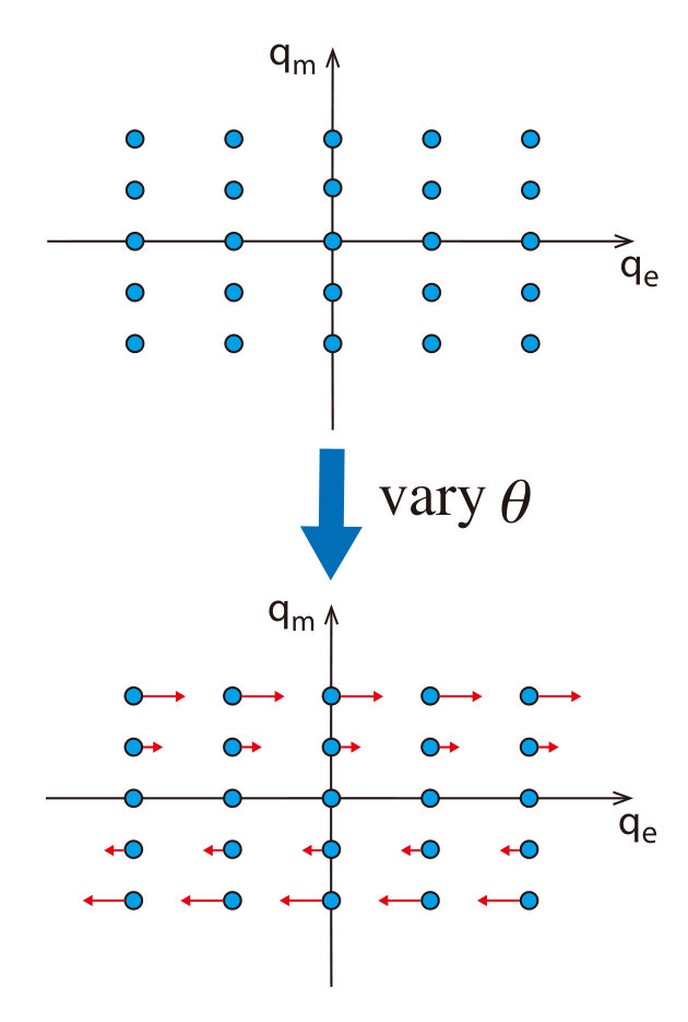 Figure 1
 Figure 2
| Anomaly class | Notation in Ref. Zou et al. (2018) | |||
Peer Reviews
No public reviews on file for this paper yet. If you reviewed it on a platform where reviews are public (OpenReview, ICLR, NeurIPS, ICML), you can paste yours below so the community can read it here.
Videos
No videos yet. Explain this paper in a talk, walkthrough, or lecture? Add one.
Fractionalization and Anomalies in Symmetry-Enriched U(1) Gauge Theories
Shang-Qiang Ning
Institute for Advanced Study, Tsinghua University, Beijing, 100084, China
Department of Physics, The University of Hong Kong, Pokfulam Road, Hong Kong, China
Liujun Zou
Department of Physics, Harvard University, Cambridge, MA 02138, USA
Department of Physics, Massachusetts Institute of Technology, Cambridge, MA 02139, USA
Perimeter Institute for Theoretical Physics, Waterloo, Ontario, Canada N2L 2Y5
Meng Cheng
Department of Physics, Yale University, New Haven, CT 06511-8499, USA
Abstract
We classify symmetry fractionalization and anomalies in a (3+1)d U(1) gauge theory enriched by a global symmetry group . We find that, in general, a symmetry-enrichment pattern is specified by 4 pieces of data: , a map from to the duality symmetry group of this gauge theory which physically encodes how the symmetry permutes the fractional excitations, , the symmetry actions on the electric charge, , indication of certain domain wall decoration with bosonic integer quantum Hall (BIQH) states, and a torsor over , the symmetry actions on the magnetic monopole. However, certain choices of are not physically realizable, *i.e., *they are anomalous. We find that there are two levels of anomalies. The first level of anomalies obstruct the fractional excitations being deconfined, thus are referred to as the deconfinement anomaly. States with these anomalies can be realized on the boundary of a (4+1)d long-range entangled state. If a state does not suffer from a deconfinement anomaly, there can still be the second level of anomaly, the more familiar ’t Hooft anomaly, which forbids certain types of symmetry fractionalization patterns to be implemented in an on-site fashion. States with these anomalies can be realized on the boundary of a (4+1)d short-range entangled state. We apply these results to some interesting physical examples.
Contents
-
III Symmetry fractionalization and anomalies in gauge theory
-
B Parametrization of 4-cocycles and classification of anomalies
-
C Hall conductivity of a (2+1)d U() symmetric invertible states
I Introduction
A three dimensional ( (3+1)d) quantum spin liquid (QSL) is an exotic gapless quantum phase. Due to the long-range entanglement inherent in this phase, it can be described by a compact (3+1)d gauge theory at low energies 111In this paper we will use the terms “ QSL” and “ gauge theory” interchangeably.. It features emergent photons as the dominant low-energy excitations, but fractional excitations (*i.e., *excitations with electric and/or magnetic charges) are still ineluctable in the system, even if they are gapped. This phase has been shown to be stabilized in a number of microscopic models Motrunich and Senthil (2002); Wen (2003); Moessner and Sondhi (2003); Hermele et al. (2004); Motrunich and Senthil (2005); Levin and Wen (2006); Banerjee et al. (2008); Shannon et al. (2012). Recently, the prospect of realizing QSLs in the “quantum spin ice” phase of rare earth pyrochlores has stured much theoretical and experimental work Castelnovo et al. (2008); Morris et al. (2009); Fennell et al. (2009); Ross et al. (2009, 2011); Savary and Balents (2012); Gingras and McClarty (2014).
Microscopic realizations of a QSL often enjoy certain global symmetries. In order to understand the physical properties of a QSL, it is important to develop a systematic theory for the interplay between these global symmetries and its more intrinsic properties due to its long-range entanglement. As an example, the quantum spin ice has a time-reversal symmetry, and the monopoles are Kramers doublets under the time-reversal transformation, *i.e., *the symmetry is realized projectively.
This understanding also provides useful information regarding the global phase diagram of a QSL, especially its proximate phases and the phase transitions between them. For instance, condensation of electric or magnetic charges can drive the U(1) QSL to a short-range entangled phase, whose nature (*e.g., *symmetry-breaking pattern) depends on the properties of the condensed charges Motrunich and Senthil (2005). Symmetry considerations are crucial in determining the properties of these proximate phases.
A given set of global symmetries can have qualitatively distinct realizations in a QSL, in the sense that QSLs with different symmetry realizations can have symmetry-protected distinctions (see Fig. 1). These different QSLs are referred to as symmetry-enriched QSLs under this symmetry.
Building on the preliminary work in Ref. Wang and Senthil (2013), gauge theories enriched by time reversal symmetry were first classified in Ref. Wang and Senthil (2016). A systematic framework for the classification of generic symmetry-enriched gauge theories was then proposed in Ref. Zou et al. (2018), and this framework was applied to obtain the classifications of some rather nontrivial examples. In this framework, the bulk properties of a symmetry-enriched gauge theory is characterized by statistics and the symmetry properties of the elementary electric charge and magnetic monopole of the theory, and its surface properties can be further enriched by weakly coupling it with a symmetry-protected topological (SPT) phase. In this paper, we will focus on the bulk properties of a symmetry-enriched gauge theory.
To completely specify the symmetry properties of a U(1) QSL, we need to know how symmetries act on the elementary electric charge and magnetic monopole, known as the symmetry fractionalization patterns. The symmetry actions on the elementary eletric charge and on the magnetic monopole are naively independent, but some of their combinations turn out to be anomalous, *i.e., *a gauge theory with certain symmetry fractionalization patterns cannot be realizable in any (3+1)d lattice spin system if the symmetry is implemented in an on-site manner, and it can only be realized as a boundary of a (4+1)d system. Ref. Zou et al. (2018) proposed a general physics-based method to detect such anomalies, and many nontrivial examples were demonstrated therein.
However, despite being general, systematic and physically intuitive, the method employed in Ref. Zou et al. (2018) can be sometimes sophisticated to implement. It is thus desirable to have a mathematical classification of anomalies, and a formula that indicates whether a symmetry fractionalization pattern is anomalous or not, and if it is anomalous, what kind of (4+1)d system can adopt this anomalous gauge theory as its boundary. Furthermore, it is desirable if this anomaly formula can be formulated purely in terms of the physical symmetry quantum numbers of the elementary electric charge and magnetic monopole.
The main goal of this paper is to develop such a systematic understanding of anomalies in symmetry-enriched U(1) gauge theories. As we will see, there are in fact two layers of anomalies: the first of them, the deconfinement anomaly, obstructs the deconfinment of the fractional excitations, rendering the notion of symmetry fractionalization ill-defined. When the first anomaly is absent, the second anomaly indicates whether the system has to live on the boundary of a (4+1)d nontrivial SPT phase. This is the more familiar ’t Hooft anomaly.
The rest of the paper is organized as follows. In Sec. II we will give a brief review of the physics of a gauge theory. In Sec. III, after sketching its derivation, we will present a classification of symmetry-enriched U(1) gauge theories and the structure of their anomalies. This analysis is based on the conjecture that all anomaly-free symmetry-enriched gauge theories can be viewed as partially gauged SPT phases. In this paper we will mostly consider gauge theories with bosonic electric charges. We will then apply the anomaly formula to some interesting examples in Sec. IV. Some of these examples were discussed in Ref. Zou et al. (2018), and our anomaly formula can reproduce the corresponding results and verify some conjectures made in Ref. Zou et al. (2018). Besides these, we also discuss some other new intriguing examples. In particular, we discuss which QSLs can be realized if SO(3) spin rotational symmetry and (3+1)d translation symmetry are preserved. Namely, we find symmetry-enriched gauge theories that can satisfy the Lieb-Schultz-Mattis (LSM) constraint. We also discuss a symmetry-enriched gauge theory that is related to the intrinsically interacting fermionic SPT phase found in Ref. Cheng et al. (2018). Finally, we conclude in Sec. V. Various appendices contain some technical details.
II Review of gauge theory
Generally a gauge theory (with bosonic electric charge) is described by the following Lagrangian at low energies:
[TABLE]
Here is the gauge coupling strength and is the axion angle. Notice that, in the absence of other symmetries, is -periodic if the charges are bosonic Vishwanath and Senthil (2013); Metlitski et al. (2013). At low energies, the theory simply describes propagating photons. Above certain energy gap, there are fractional excitations carrying electric and magnetic charges. We denote the electric and magnetic charge of an excitation by and , respectively. Due to the Dirac quantization condition Dirac (1931), the possible values of and form a charge-monopole lattice. Because of the -term, an excitation acquires a “polarization charge” due to the Witten effect Witten (1979) (see Fig. 2). Therefore, the charge of a generic fractional excitation should be written as , where is an integer counting the electric charge of this excitation at . The self-statistics of a fractional excitation with electric and magnetic charges is given by . This formula indicates that the statistics of the excitations is invariant when is changed by .
In the absence of any orientation-reversing symmetries (time reversal and/or spatial reflection), can be tuned continuously. Without loss of generality, in this case we can always tune to be [math] without encountering a phase transition. In the presence of an orientation-reversing symmetry, is quantized to be an integer multiple of . In all these cases, there is a charge-neutral monopole with a unit magnetic charge, i.e., . If with even (odd), the elementary charge-neutral monopole is bosonic (fermionic). We will denote by the elementary electric charge with , denote by the elementary charge-neutral monopole with . The charge-monopole lattice is generated by and , and we call bound states of certain numbers of and a dyon.
For , the gauge theory has an emergent duality symmetry group of automorphisms, *i.e., *permutations of fractional excitations that preserve all universal properties, such as exchange statistics. In defining automorphisms we ignore energetics such as gaps of the particles. Permutation of charges can be specified by its action on the two generators:
[TABLE]
Clearly . In order to preserve the charge-monopole lattice, we must demand . One can further show that only preserves the geometric Berry phase associated with braiding dyons, while flips the Berry phase. All integer matrices with unit determinant form the group SL, generated by and :
[TABLE]
However, the transformation changes the statistics of particles for odd (*e.g., *a bosonic charge turns into a fermionic dyon ), so the group that preserves all Berry phases is actually generated by and , and we will denote this group by . with odd can only be realized in a U(1) gauge theories with fermionic charge, and we will not discuss them in this paper.
We can also consider the permutations reversing the sign of the Berry phase, which must correspond to orientation-reversing transformations. All these can be obtained from by multiplying the following matrix
[TABLE]
We will denote all such permutations by .
Altogether, we have found the duality symmetry group .
Although we started from the relativistic Lagrangian Eq. (1), our discussion below will not rely on Lorentz symmetry in essential ways. In other words, we consider more broadly quantum phases with emergent U(1) gauge symmetry with gapped electric and magnetic charges, which are not necessarily described by the relativistic Lagrangian.
III Symmetry fractionalization and anomalies in gauge theory
Now we consider a gauge theory realized in a microscopic model with a global symmetry group . We will analyze how global symmetry transformations are realized in the low-energy theory. For clarity, let us assume that is internal, and we expect the results for spatial symmetries will be similar Thorngren and Else (2018); Zou (2018). We will also consider the case where includes lattice translation symmetry in some occasions. Notice that may contain both unitary and anti-unitary transformations. To formally keep track of this, we define a grading on to indicate whether a group element corresponds to a unitary () or anti-unitary () transformation.
First of all, we consider how gauge-invariant operators transform under the symmetries. In the low-energy limit of a gauge theory, all gauge-invariant local operators can be built up out of field strengths and . They may transform nontrivially under a symmetry operation. For example, a charge conjugation symmetry takes and . Equivalently, because and are sourced by electric and magnetic charges, we can also directly write down how the types of electric and magnetic charged excitations transform. In the example of charge conjugation, and . Clearly such a transformation is an element in . Therefore, we have a group homomorphism from to (preserving the grading ).
When is given, we still do not have a complete description of the symmetry action. The missing information is how symmetry acts locally on an individual fractional excitation, which will be referred to as symmetry fractionalization. A major goal of this work is to obtain a complete classification of both and symmetry fractionalization in physical gauge theories. The basic principle is the following conjecture, first formulated in Ref. [Zou et al., 2018]:
All physical symmetry-enriched gauge theories can be realized as partially gauged SPT phases.
Let us elaborate on this statement. By physical, we mean that the gauge theory can be realized in a 3D microscopic model with an on-site symmetry group . The above conjecture allows us to only consider SPT phases whose symmetry group contains as a normal subgroup, which after gauging becomes the gauge symmetry. is the remaining global symmetry after gauging. We note that the above principle has also been applied to study symmetry-enriched SU gauge theories Guo et al. (2018); Wan et al. (2019).
An immediate consequence of this conjecture is that one should be able to identify a certain dyonic excitation (and multiples of this dyon) as the matter of the SPT phase, coupled to a gauge field. In the charge-monopole lattice, all the matters of this SPT phase should correspond to a line of lattice points passing through the origin. The global symmetry must fix this line in order for the gauging to make sense. Denote a dyon on this line by , and suppose the symmetry transformation on the charge type is given by , then
[TABLE]
where is a nonzero integer. To have a non-zero solution to this equation, we must have
[TABLE]
Together with , we find . Since , the only consistent choices are , corresponding to . In other words, such SL(2, ) matrices have trace . It is known that they are actually all conjugate to for . Because all such transformations have an infinite order except for , when is a compact group (including finite groups) we only need to consider , *i.e., *the charge-conjugation subgroup. When contains an infinite-order element (*e.g., *lattice translation), the element can act as the transformations. If the symmetry is realized with , we can take any of the dyons as the SPT matter. If the symmetry is realized with , we should take as the SPT matter.
We can also consider anti-unitary transformations, which have . Following a similar argument, we find that if there is a fixed line in the charge-monopole lattice, the trace must be [math], i.e., . One can show that all such matrices are conjugate to either or . The former case is just the usual convention that the electric (magnetic) fields are even (odd) under time reversal. In the later case, is the fermionic dyon identified as the SPT matter. This case corresponds to a gauge theory with . We will not consider this case further in this work.
To conclude this discussion, if we only consider compact symmetry groups, we may restrict the image of to the charge-conjugation subgroup of .
Next we analyze symmetry fractionalization.
III.1 Symmetry fractionalization
Based on the above discussion, in a gauge theory a general compact symmetry group comes with a -grading . means acts as charge conjugation:
[TABLE]
Besides the charge-conjugation grading, there is also the grading to distinguish unitary and anti-unitary transformations. We will take the convention that the electric and magnetic fields transform as
[TABLE]
So the transformation belongs to . Equivalently, the charges transform as
[TABLE]
Once we specify how charges are permuted by symmetries, we examine how symmetry locally transforms an individual charge. Consider the action of the global symmetry operator for on a physical state with multiple fractional excitations which are spatially well-separated. The symmetry operator may transform the field lines induced by the charges, as given in Eq. (8). In addition, may also induce localized unitary transformations on each of the charges. We argue that
[TABLE]
Here we separate local unitary transformations from the non-local transformation that acts globally on gauge theory. This equation should be understood as an (approximate) operator identity when operators localized in the neighborhood of charge excitations are concerned.
Comparing the global symmetry action and yields
[TABLE]
where has its nontrivial action localized within the vicinity of , and we have used the fact that and the fact that operators whose nontrivial actions are localized in different regions commute with each other.
Comparing this with , we must have
[TABLE]
and
[TABLE]
In particular, .
Now we consider the associativity:
[TABLE]
So we have the associativity constraint
[TABLE]
There is some redundancy in due to the freedom to redefine by multiplying a phase to it. In order to not affect , they need to satisfy . This redefinition of local operators changes the phases in the following way:
[TABLE]
Now let us specialize to and . For , , therefore
[TABLE]
defines a -cocycle in , where the subscript indicates that acts on as identity/complex conjugation if or . The redundancy in Eq. (15) means that the equivalence classes of are given by the second cohomology group , which in the literature is also denoted as , where the subscript indicates that the action of time reversal is given by . A brief review of these mathematical concepts is provided in Appendix A.
Similarly, we can show that is classified by , where the subscript indicates that acts on as identity/complex conjugation if or . So different symmetry fractionalization classes can be labeled by two -cocycles and . In Ref. Zou et al. (2018), and are dubbed the electric and magnetic projective representations of the symmetry group , respectively.
Notice that in the absence of any orientation-reversing symmetry, the properties of the monopole can be changed by smoothly varying . To understand the effect of the -term, let us start with , where in our convention is a boson with a certain projective quantum number . To get to the case with a nonzero , we can imagine continuously tuning the value of , so that the positions of the fractional excitations in the charge-monopole lattice are shifted due to the Witten effect (see Fig. 2). To have a charge-neutral elementary monopole, we need to tune the value of to be an integral multiple of , say, with an integer. Then the projective quantum number of the charge-neutral elementary monopole with this value of is determined by the excitation with at , which is (this is well-defined since for an orientation-preserving symmetry both and are classified by ). In particular, when is varied by , the statistics of the monopole is invariant, but its symmetry fractionalization pattern gets shifted by . So in this case is well-defined only up to .
In the presence of an orientation-reserving symmetry, is quantized to be a multiple of . In this case, we can still define the symmetry fractionalization class of charge-neutral monopoles (not just up to ).
This discussion can be generalized to other duality transformations, e.g. the transformation, as long as they are compactible with the symmetry action on charge types. Two symmetry fractionalization classes related by these duality transformations should correspond to the same symmetry-enriched phase. For example, if is unitary and acts as identity or charge conjugation, the transformation commutes with the symmetry action, so in this case the electric and magnetic projective representations can be interchanged without changing the phase.
Therefore, following general considerations, we have found that a symmetric gauge theory is equipped with 4 pieces of data: symmetries permuting charge types, given by , and projective symmetry transformations, parametrized by , the value of , and . However, it is not clear that every can be realized physically in (3+1)d as a partially gauged SPT phase. In fact, it is sometimes even problematic to discuss the classification of projective quantum numbers if action of contains e.g. elements. Below we address this issue.
III.2 Ungauging
We would like to construct a U(1) gauge theory from gauging a bosonic SPT phase. First, we must identify the matter particles, or “gauge charges”. Suppose that the matter is generated by a particular dyon . Without loss of generality, we may assume . We will further assume that , so the dyon is bosonic. Then we perform a duality transformation so that this dyon becomes the charge . More explicitly, the duality transformation takes the following form:
[TABLE]
with . It is straightforward to check that . The “monopole” is actually the image of under this duality transformation. Notice that since are not uniquely determined, there are infinitely many choices of the “monopole”, which are related to each other via transformations. From now on, we will assume that such a duality transformation has been done, so that the matter is generated by the bosonic charge, and there is a charge-neutral elementary monopole . In the absence of any orientation-reversing symmetry, will always be taken as a boson, because this can be achieved by smoothly tuning to be 0. On the other hand, in the presence of a orientation-reversing symmetry, the value of cannot be smoothly varied and the statistics of is a robust universal feature of this symmetry-enriched phase.
We now determine the structure of the symmetry group of the matter. In the gauge theory, the charge can transform projectively under , with a factor set that specifies the corresponding projective representation. Correspondingly, in the SPT phase the fundamental charge- boson carries the same projective representation of . Mathematically, it means that the actual symmetry group of the SPT phase is an extension of by (while the symmetry group of the gauge theory is of course just ). For notational convenience we use and its isomorphic group interchangeably, i.e., is identified as . Let us now define . Denote the unitary transformation associated with by , and let be a rotation. We have the following relation:
[TABLE]
Because charged bosons transform as projective representations of , we have
[TABLE]
These two relations Eqs. (18) and (19) completely determine the group structure of . In the following it will be more convenient to use additive notations for group multiplication, and label elements of as where and . The multiplication in is then given by
[TABLE]
with .
It is now well-understood that the classification of bosonic SPT phases in and spatial dimensions is given by group cohomology Chen et al. (2013), plus additional “beyond cohomology” phases when anti-unitary symmetries are present in 3D given by Vishwanath and Senthil (2013); Xiong (2018); Gaiotto and Johnson-Freyd (2019). For compact (or finite) , we have . The “beyond cohomology” part is not relevant for our purpose, because and describes SPT phases protected by alone. Below we present an explicit description of .
III.2.1 Projective quantum numbers of monopoles
Before discussing the general classification, we first explain how the symmetry properties of the magnetic monopole is encoded in this formalism.
Let us start from the simplest case where is unitary and . In this case, . The Künneth formula then implies
[TABLE]
The last equality assumes a compact/finite . Physically, describes SPT phases protected by alone and thus is not of interest. The other factor, , describes projective representations of and it is very natural to identify it with the fractionalization class of magnetic monopoles. In fact, we can find the following explicit parametrization of -cocycle in :
[TABLE]
Here must be a -cocycle of , and is a -cocycle in .
We will show that the -cocycle indeed encode the symmetry fractionalization pattern on the monopole, *i.e., *it is equivalent to . To do so, let us first turn on the gauge field. In the group-cohomology models with a unitary symmetry group, a -cocycle in fact determines the space-time partition function on a general -manifold Kapustin (2014), equipped with background gauge fields 222When the symmetry group is finite, such a partition function can be rigorously represented as a finite state sum on a triangulated manifold. Although in our case the symmetry group contains and more work is needed to rigorously write down the partition function, we will dispense mathematical rigor for now and proceed formally.. Since the SPT phase is gapped and we are only interested in the topological part of the response theory, we can assume that the gauge fields are flat. Denote the partition function of the SPT phase on a closed space-time manifold equipped with the background gauge field, represented by a -valued 1-cochain , and gauge field , by . The expression of is determined by Eq. (22), and it is given explicitly in Eq. (24). If is promoted to be a dynamical gauge field, then the partition function in the presence of a background gauge field is
[TABLE]
where includes both the Maxwell term and the -term , which contains no coupling between and . All coupling between and is in the topological term:
[TABLE]
Here is the -valued 3-cocycle on which is the pull-back of by the map corresponding to the gauge field . This is essentially equivalent to Eq. (22). Notice in writing the above action, we have dropped terms that only depend on (and ). These terms physically describe attaching a -SPT to the gauge theory, and they will not be considered in this paper.
Now using the correspondence between and , we write with where is the Bockstein homomorphism. Using integration by parts we find
[TABLE]
Here is the field strength. Formally this action is analogous to the well-known topological theta term, and it will potentially give the monopole nontrivial projective quantum number under .
To fully unearth the physical consequence of , we put the theory on , with containing only spatial components and a general space-time -manifold, and put a flux through (i.e., encloses a unit monopole). We then take a limit where the linear size of is much greater than that of the . Now this partition function describes the quantum amplitude of a process in which a monopole moves in the reduced spacetime . This quantum amplitude receives contributions from both and the -term. The contribution from the -term is analyzed above in Sec. III.1: the -term can change the projective quantum number of the monopole by . The contribution from becomes . This means that the worldline of the monopole is further associated with an additional contribution to the quantum amplitude, , which is precisely the partition function of a (1+1)d -SPT state whose boundary realizes the projective representation specified by the factor set . That is to say, the magnetic flux line is further decorated with this (1+1)d -SPT state, and its end point, the magnetic monopole, gets one more piece of contribution to its projective representation of , which is specified by the factor set . So when both the -term and the are taken into account, the projective quantum number of the charge-neutral monopole is given by for . In the present case, and is just identified as .
III.3 Structure of
Now we explain the main result of this work, the structure of the cohomology group . Details of the proofs of our statements can be found in the Appendix B.
Recall that is an extension of by , with a -cocycle . A cohomology class in is specified by three layers of data:
A 1-cocycle from , where the coefficient is in fact . In other words, satisfies . Importantly, and need to satisfy an obstruction-vanishing condition: Define
[TABLE]
Here represents the fractional part of with respect to , i.e., and . One can easily show that is a 3-cocycle in . There must exist such that , where . Namely, needs to be a trivial cocycle in for this obtruction to vanish. We will call the deconfinement obstruction (or symmetry localization obstruction) class, for reasons that will become clear later. We remark that this obstruction class is purely determined by (how the symmetry permutes fractional excitations), (the symmetry actions on the electric charge ), and , whose meaning will be explained below. In contrast, the symmetry actions on the magnetic monopoles are not in charge of this obstruction, as will be clear later. 2. 2.
When the deconfinement obstruction vanishes, we can solve , and different solutions of are parametrized by a torsor over . When , the obstruction class is canonically zero, and we have shown that describes projective representation carried by magnetic monopoles in Sec. III.2.1. Based on the mathematical structure, we conjecture that the same interpretation holds more generally, namely, the torsor classifies symmetry fractionalization on monopole excitations. 3. 3.
Finally, an obstruction -cocycle must vanish. Otherwise, the gauge theory that would arise from gauging this SPT phase must be realized on the boundary of a (4+1)d SPT phase defined by . When is trivial, we may modify the 4-cocycle by an element from , corresponding to stacking a G-SPT phase. Notice that this does not necessarily lead to a new symmetry-enriched gauge theory Wang and Senthil (2016); Zou et al. (2018). The full expression for is rather complicated and is given in Eq. (106) of Appendix B. Below we will consider in detail specific cases where the formula simplifies significantly.
To better understand the classification, we consider a few simplified cases.
Case 1: If is unitary and compact (finite), then , so we can set , which implies that the obstruction class vanishes identically. In this case, the 4-cocycle has the following simple representation:
[TABLE]
As before, is a 4-cocycle in , and can be taken as a 3-cocycle in .
As before, the 3-cocycle encodes the information of the symmetry fractionalization class on the monopole. Using and , which characterizes the symmetry fractionalization class on the charge, we have the following expression for the obstruction -cocycle:
[TABLE]
We claim that a gauge theory with symmetry fractionalization pattern given by , and is realizable if and only if belongs to the trivial class in . If belongs to a nontrivial class in , then this gauge theory is anomalous, and can only be realized on the boundary of a (4+1)d G-SPT characterized by the 5-cocycle . We will provide further arguments for this statement in Sec. III.5.
Case 2: For a general finite/compact group that contains anti-unitary elements, we have . It is not difficult to show that must take the following form:
[TABLE]
with an integer. Even (odd) represents the trivial (nontrivial) class of . Let us further assume for simplicity, and consider the following 4-cocycle
[TABLE]
Here is given by
[TABLE]
We note that describes a bosonic integer quantum Hall (BIQH) state of Hall conductance . The expression for can be found in Appendix B. Eq. (30) is not the most general form of 4-cocycle in this case, but the following explanation holds more generally.
We claim that this -cocycle with given by Eq. (29) corresponds to . To see it, consider the slant product of over (see Appendix A for a brief introduction of slant products):
[TABLE]
It is well-known that the slant product corresponds to dimensional reduction of the system onto a domain wall Wang and Levin (2015). Eq. (32) means that the quantum state on a domain wall labeled by can be described by the data . From Eq. (29), we see that when , , the slant product gives and this domain wall is a trivial state. On the other hand, when , , and the domain wall is a bosonic integer quantum hall state with (in units of ) 333Notice when a coboundary transformation on is performed, can change by , the 3-cocycle that describes a BIQH state with . This precisely reflects the fact that the states with and with are in the same phase in the absence of any symmetry other than and time reversal.. This exactly matches the properties of a state with Senthil and Levin (2013); Vishwanath and Senthil (2013); Xu and Senthil (2013). So, intuitively, the 4-cocycle can be interpreted as decorating (2+1)d BIQH states onto time-reversal domain walls, classified by . We should emphasize that this relation between and only holds for anti-unitary symmetry . If is unitary, in general there is no such relation between and the -term. Also, notice that Eq. (29) only holds for compact/finite symmetry groups, and it does not hold for symmetries like lattice translations, which will be discussed next.
Case 3: For lattice translation symmetry along the direction, , we have , and can take any integral value. We call the element that translates the system by one lattice spacing along the direction. Again consider the 4-cocycle given by Eq. (30), and now the meaning of the slant product Eq. (32) is that on each plane perpendicular to the direction, we have a BIQH with Cheng et al. (2016). Therefore, is a more general concept than the value, and it indicates certain domain wall decoration with BIQH states. In this case of translation symmetry, in the corresponding gauge theory the action of translation is Williamson et al. (2019). To see this, consider a magnetic monopole in the system. When the monopole is translated by one unit along , say from below to right above , the magnetic flux through the plane changes by . The quantum Hall response then creates charge- on the plane. As a result, the under the monopole transforms as
[TABLE]
That is, this translation transformation is in fact . We notice that the theory obtained by gauging the U(1) symmetry of an infinite stack of BIQH states has unconventional low-energy dynamics, as the photon dispersion is no longer linear Williamson et al. (2019). Therefore it can not be described using the relativistic Lagrangian Eq. (1) 444 transformation is not an explicit symmetry of the relativistic theory (1).
III.4 obstruction class
Having discussed the meaning of and , we now further elaborate on the obstruction class.
First of all, if is a finite group or a compact Lie group, the general form of is given by Eq (29). When is unitary, and for all , so the obstruction class vanishes.
Now consider a general , *i.e., *the symmetry group may contain anti-unitary elements. It turns out that even for a general , the obstruction also vanishes identically. To see it, define . It is straightforward to show that , so vanishes.
Let us demonstrate why this is the case physically by considering an example with , where is unitary and finite. We denote the group element of as , and . Let us also suppose that entirely comes from . We choose as in Eq. (29) with . We will also set in this example. Notice so far we have only specified the data responsible for the obstruction class, and our discussion is independent of the possible presence of the obstruction class.
A -SPT phase can always be obtained by first breaking the symmetry and making the system a superfluid, and then proliferating the vortex lines of this superfluid. In order for such a gapped state to exist, a vortex line to be proliferated must be fully gapped without any degeneracy or gapless modes.
Since , a BIQH state is decorated onto a time-reversal domain wall. Suppose we thread a flux through the domain wall. Due to the quantum Hall response, the flux threading creates a charge- excitation, which carries a projective representation labeled by . In other words, on a flux line a domain wall binds a “zero mode” protected by the symmetry (in this example, ) when is nontrivial. Naively, this poses an obstruction to proliferating vortex lines to yield a gapped symmetric state, as the proliferation seems to break the symmetry.
However, we are allowed to decorate the vortex lines to be proliferated with gapped 1D states. In this example, we can just decorate the vortex lines with a 1D -SPT phase with a factor set . Due the time-reversal symmetry domain wall, the two sides on the vortex lines have 1D SPT states labeled by and , with a projective representation sitting on the domain wall and neutralizing the projective representation arising from the Hall response. Now everything is gapped, and it is possible to proliferate the vortex lines to get a symmetric gapped state, if the obstruction class further vanishes. In fact, as long as no symmetry acts as -transformations, the corresponding (3+1)d symmetry-enriched gauge theory can at most suffer from an obstruction, and it can always be realized on the boundary of a (4+1)d invertible state Zou et al. (2018) (see Appendix C therein), which can be constructed via a generalization of the layer construction in Ref. Wang and Senthil (2013).
Now we give an example where the obstruction class is actually nontrivial. We choose the symmetry group to be . Notice this is not a compact/connected Lie/finite group. Denote the generator of by . Consider an example with . To see whether the obstruction class is nontrivial in this case, we compute the slant product . As long as is nontrivial, the obstruction class is nontrivial.
To have a concrete example, suppose with (or its finite subgroup ). If we take to be the fundamental representation of (the generating element in ), then in order for the obstruction class to vanish, we need
[TABLE]
We can interpret the as lattice translation. As explained in the previous section, such a -SPT phase can be viewed as a stack of 2D BIQH phases with Hall conductance . However, since the matter boson carries the fundamental representation of SU, the Hall conductance is constrained to be a multiple of () when is even (odd) (see Appendix C for derivation). This is exactly the condition that the obstruction class vanishes.
If takes any other integer value, then the obstruction class is nontrivial, which means the state with those other values of are not valid -SPTs. Let us understand what is wrong with those states. Suppose such a state could be realized, then we can gauge the symmetry to obtain a gauge theory. After gauging, whenever a magnetic flux line goes through a plane of such a BIQH state, charge- will be left on the plane due to the nonzero Hall conductance. This charge- object carries projective representation of the PSU symmetry, thus resulting in symmetry-protected degeneracy (gapless modes) on this magnetic flux line. Note that in this case we cannot cancel the degeneracy by attaching (1+1)d PSU SPT state on the magnetic flux line. In a gauge theory, the magnetic flux lines need to be “condensed” for the monopoles to be deconfined. However, the presence of the gapless modes makes these flux lines visible, and, as a result, the monopoles cannot be viewed as deconfined excitations, which contradicts our assumption that this state can be gauged to yield a gauge theory. For this reason, we refer to the obstruction as the deconfinement obstruction. Because now the monopoles are not deconfined excitations, it does not make sense to talk about localizing symmetry actions on them, and such an obstruction can also be called a symmetry localization obstruction.
So what sort of (4+1)d bulk can support such an (3+1)d SPT phase on the boundary? To answer this, let us first ask what sort of (3+1)d bulk can support on its boundary a BIQH with violating the constraint given in Eq. (34). In Appendix C, we show that a (3+1)d bulk with the following -term in the response can produce the desired response on its (2+1)d surface:
[TABLE]
Strictly speaking, the U(1) gauge field needs to satisfy additional conditions to reflect the fact that charges carry projective representations of PSU(), see Appendix C and Sec. III.5 for for details. This type of (2+1)d states are referred to as anomalous invertible states Wang et al. (2019). Namely, this invertible state can only exist on the boundary of a higher-dimensional trivial bulk. If we try to gauge the U(1) symmetry in the anomalous invertible state, the dynamical gauge field resulting from gauging also has to be extended into the bulk.
Now we come back to the 3D stack of the 2D anomalous BIQH states, and ask on the boundary of what kind of (4+1)d bulk this (3+1)d stack can be realized. Apparently, the (4+1)d bulk that supports the anomalous (3+1)d invertible phase must also contain topological terms. Suppose the (4+1)d space-time manifold is . Formally, if we introduce a gauge field , the bulk response is given by
[TABLE]
If we place the (4+1)d theory on , and let , the partition function then yields the following theory living on a “flux surface” (or the worldsheet of a “monopole” loop in four spatial dimensions):
[TABLE]
As we explain below, because electric charges carry projective representations, we need to identify , where is the background PSU bundle, and is the characteristic class that describes the obstruction of lifting a PSU bundle to SU() bundle. So the action is essentially , which describes the Lieb-Schultz-Mattis anomaly of a (1+1)d PSU-symmetric spin chain, where each site transforms as the projective representation labeled by Yao et al. (2019), as expected from the physical argument presented earlier as the flux surface terminates on a flux line on the (3+1)d boundary. Indeed, these PSU-symmetric spin chains live on the boundary of (2+1)d SPTs classified by , which is also the classification of the anomalies here.
From this example, we see that a natural way to resolve a non-vanishing deconfinement obstruction is to require that both the background gauge field and the dynamical gauge field be extended to the higher-dimensional bulk, and is therefore quite different from the usual ’t Hooft anomaly. This is similar to the symmetry-localization obstruction found in (2+1)d symmetry-enriched topological phases Barkeshli et al. (2019); Tarantino et al. (2016); Fidkowski and Vishwanath (2017); Barkeshli and Cheng (2018).
III.5 ’t Hooft anomaly formula
Before finishing this section, we will sketch an informal derivation of the ’t Hooft anomaly formula in the special case where for all , which also explains the physical meaning of the object given by Eq. (28). We will limit ourselves to the case .
Suggested by the explicit parametrization, we postulate that the topological response theory of the to-be-gauged SPT takes a form similar to Eq. (24):
[TABLE]
While we still use the notation to represent the background gauge field, we must keep in mind that is generally not a direct product of and . In particular it means that one has to modify the flat connection condition to
[TABLE]
Here is the pull-back of the group -cocycle to the bundle.
The response has to be gauge-invariant. Under a gauge transformation, is shifted by where is a 1-cochain, and is shifted by . We do not need to know the specific forms of and . In order to preserve the flatness of the gauge field, must be shifted to . Therefore, the topological response theory changes by
[TABLE]
Here we used . Thus the theory is not gauge-invariant. But the variation is now seen to only depend on the gauge field. This suggests that we fix the problem by including a 5D bulk whose boundary is , with the following action:
[TABLE]
Here is an extension of the gauge field to . Notice this (4+1)d response theory is essentially Eq. (28).
Let us check that the variation of under a gauge transformation does give Eq. (40):
[TABLE]
Thus this term exactly cancels Eq. (40).
Therefore the whole theory (5D bulk and 4D boundary) is gauge-invariant. Since the 5D bulk response only depends on the gauge field, it describes a -SPT phase. This result means that the U(1) gauge theory obtained by gauging the -SPT described by the 4D action Eq. (38) can live on the boundary of a 5D -SPT phase described by Eq. (41).
IV Applications
In this section we will apply the anomaly formula to various examples. In all these examples, the deconfinement obstruction class always vanishes.
IV.1
Let us first consider gauge theories enriched by a unitary symmetry. The extension of by is given by
[TABLE]
Physically, means that the symmetry acts as a charge conjugation, and means that it does not act as a charge conjugation.
For the case with , because , there is no nontrivial symmetry fractionalization pattern, and there is only one possible gauge theory with no fractionalization on or . This state is denoted by in Ref. Zou et al. (2018).
Below we will study the case. A representative 2-cocycle is:
[TABLE]
with . In the notions of Ref. Zou et al. (2018), the cases with , or , and are denoted as , and , respectively.
Let us compute the obstruction -cocycle. From we find the only non-zero component of :
[TABLE]
Then using the formula Eq. (28) we have
[TABLE]
This is a nontrivial 5-cocycle if and only if . So and are anomaly-free, while is anomalous and must be realized on the boundary of a (4+1)d group-cohomology SPT phase. Indeed, there is a (4+1)d group-cohomology SPT phase, and our result implies that can be its boundary state. These results agree with Ref. Zou et al. (2018).
We notice that in (4+1)d there is a “beyond-cohomology” SPT phase Wen (2015). The boundary of this phase is characterized by a mixed -gravity anomaly. We now argue that the boundary can not be a -symmetry-enriched U(1) gauge theory. First of all, we may restrict to U(1) gauge theories with both electric and magnetic charges bosonic (the other possibility, the so-called all-fermion electrodynamics, has global gravitational anomaly). Since the symmetry is , it either acts trivially or as charge conjugation on charge types, as these are the only order-two elements in the duality group. Under these conditions, all possible -symmetry-enriched U(1) gauge theories have been exhausted here, therefore we conclude that this “beyond-cohomology” SPT phase cannot have a U(1) gauge theory as symmetry-preserving boundary termination.
IV.2
Let us now consider an example of an anomalous U(1) QSL with SO(3) spin rotational symmetry. Ref. Zou et al. (2018) shows that the state , where both and are bosons that carry spin-1/2, is anomalous.
Now we apply our obstruction formula to re-derive this result. It suffices to show that this state is still anomalous when the SO(3) symmetry is broken down to its subgroup, consisting of three rotations around and axes. This is the minimal subgroup of SO(3) where the spin- projective representation still makes sense, since . In the anomalous theory, both and carry the nontrivial projective representation of . Ref. Zou et al. (2018) suggested that this state is still anomalous, and we indeed find that the obstruction class is nontrivial, thus verifying this statement. The details will be postponed to Sec. IV.5.
IV.3
Next we consider the symmetry group . This symmetry is relevant for experimental QSL candidates made of non-Kramers quantum spins. Ref. Zou et al. (2018) found 75 symmetry fractionalization patterns for gauge theories with this symmetry, where 38 of them are anomaly-free and the other 37 are anomalous. We will apply our anomaly formula to rederive the anomalies of the 37 anomalous states, and we will also confirm a conjecture made in Ref. Zou et al. (2018) about the anomaly classes.
Let us denote where is the generator of the subgroup and the generator of the subgroup. They satisfy . The homomorphism is determined by . We can then systematically classify fractionalization classes (see Appendix D for details).
Let us consider how to distinguish cohomology classes in . Applying Künneth formula, we find
[TABLE]
Given a -cocycle , we can decompose the cohomology class in the following way:
[TABLE]
where , and is the generating class of , for , for . corresponds to (4+1)d SPT phases protected by alone, which is precisely the state whose boundary can be (see Sec. IV.1). Below we will focus on the remaining part.
We now discuss how to determine , from . We consider first, which turns out to be simpler to define. We use a cohomology operation called slant product, which for each group element defines a group homomorphism (see Appendix A.3 for a review). We define .
To find , we need a generalization of slant product, 2-slant product, which are defined now for multiple group elements, see Appendix A.3. We define
[TABLE]
Using the definition of 2-slant product in Appendix A.3, one can check that both and are invariants for the cohomology class (*i.e., *invariant under coboundary transformations).
We compute the obstruction classes when both and are nontrivial (when either of them is trivial the obstruction class vanishes automatically). The result is tabulated in Table 1.
Ref. Zou et al. (2018) indeed found that all the 6 states we consider here are anomalous. In fact, after exhausting all possible symmetry fractionalization patterns of this symmetry, Ref. Zou et al. (2018) found in total 37 anomalous symmetric gauge theories. Furthermore, the arguments therein (see Sec. VII C of Ref. Zou et al. (2018)) imply that, to show the anomalies of all these 37 states, it actually suffices to show that , and are anomalous, which we have shown here. Therefore, we have reproduced the results in Ref. Zou et al. (2018) on anomalous symmetric gauge theories.
Ref. Zou et al. (2018) also conjectured a classification of the anomaly classes of these 37 anomalous states, within each class the anomaly of the states are the same. Our results also confirm this conjecture. More precisely, there are 6 anomaly classes (see Ref. Zou et al. (2018) for the properties of these states):
, , , , , , .
- 2.
, , .
- 3.
, , .
- 4.
, , , , , , , , .
- 5.
, , , , , , , , .
- 6.
, , , , , .
IV.4 Lieb-Schultz-Mattis-Hastings-Oshikawa anomaly
We now apply our results to systems in which Lieb-Schulz-Mattis-Hastings-Oshikawa (LSMHO) type theorems Lieb et al. (1961); Oshikawa (2000); Hastings (2004) hold. For concreteness, consider a translation-invariant lattice with spin- per unit cell, whose symmetry group is SO(3). The LSMHO theorem states that such a system does not allow a non-degenerate ground state preserving all symmetries on a torus. Such a constraint can be understood as the manifestation of a particular ’t Hooft anomaly, if we view this lattice system as the boundary of a (4+1)d crystalline SPT “bulk” that consists of a stack of Haldane chains in the 4th dimension Cheng et al. (2016); Jian et al. (2018); Huang et al. (2017); Metlitski and Thorngren (2018). We will refer to this anomaly as the LSM anomaly. Our goal is to understand the implication of such an anomaly in a U(1) gauge theory.
Let us first explicitly write down the “bulk” theory for the LSM anomaly. While the protecting symmetry involves lattice translations, we will nevertheless treat them formally as an internal symmetry and imagine coupling the bulk to gauge fields of the translation symmetries , denoted by for translations in the three orthogonal directions. We also turn on a background SO(3) gauge field . The bulk response theory takes the following form Metlitski and Thorngren (2018):
[TABLE]
Here is the Stieffel-Whitney class of the SO(3) bundle .
Let us see how this anomaly can be resolved by a gauge theory. Notice that for because SO(3) is connected. For translations, let us for simplicity assume that act on the charges in the same way, denoted by :
[TABLE]
This is natural if the cubic rotation symmetry is preserved. As shown in Sec. III, there are three possibilities of how translation is associated with the duality transformation of a gauge theory: the translation acts as the identity, the charge conjugation, or the transformation.
First we present an argument to rule out . We calculate the fractionalization classes using the Künneth decomposition:
[TABLE]
The first factor of the above equation indicates that charges can transform as spin-’s under SO(3). The factor represents magnetic translation algebra in or planes. However, we should notice that each of these phase factors is a continuously tunable phase factor, and therefore should not form distinct fractionalization classes. This is similar to theta terms in topological response.555Mathematically, this is the distinction between deformation classes and not just isomorphism classes. We conclude that when the fractionalization class of the translation symmetry is completely trivial, and thus can not happen in the presence of LSM anomaly, and, as a result, the translation must be mapped to a nontrivial element in the duality group.
Next let us consider being the charge conjugation. In this case, we find
[TABLE]
So there is only one nontrivial translation symmetry fractionalization pattern. An invariant that characterizes the fractionalization class is
[TABLE]
To resolve the LSM anomaly, clearly one of and has to carry spin-, because the “background matter fields” carry spin-1/2. Without loss of generality, let carry spin-. It is natural to expect that needs to carry the nontrivial translation symmetry fractionalization. We show in Appendix E that this symmetry fractionalization pattern indeed realizes the LSM anomaly correctly. In contrast, the LSM anomaly cannot be realized if none of and carries spin-1/2, or none of them carries the nontrivial translation fractionalization pattern. The general condition for a QSL to satisfy the LSM constraint due to these symmetries is given by Eq. (141).
Let us list the possible symmetry-enriched QSLs that can be realized in a lattice with spin- per unit cell. As before, we denote the one with spin- as , the spinon. Then must carry integer spin, otherwise the state suffers from the SO(3) anomaly. There are only two types of QSLs that satisfy the LSM constraint: and , where ‘’ means that the translation symmetry acts as charge conjugation, means a spin-1/2 boson, and means a boson with nontrivial translation fractionalization. In Appendix F, we show that both of them can indeed be realized by explicit parton constructions.
On the other hand, if the lattice has an integer spin per unit cell, then the possible symmetric QSLs are and .
Lastly, we consider the possibility that is realized as for some nonzero integer . Leaving a general classification of this case for future work, here we will briefly describe an example where one of the translations, say , is mapped to . To this end, we use a fermionic parton construction to write the spin operator in terms of Abrikosov fermions: , with the local gauge constraint imposed. We then put the fermions into the a mean-field state described by a non-interacting Hamiltonian. The original spin system is recovered by coupling the fermions to gauge field. For our purpose, we choose the following mean-field band structure: for all fermions on a given plane, we make and both have the same Chern band with Chern number . Together they form a band, which is the minimal required by the SU(2) spin symmetry (see Appendix C). In this case, the translations do not change the fermionic gauge charge. Following a similar discussion in Sec. III.3, it is easy to see that implements the transformation.
It is also possible to have a QSL where all three translations act as . To construct such a state, one just needs to take three copies of the above state and make them rotationally symmetric, and turn on hybridization between the charges in these three gauge theories. The resulting theory is an SO(3) and translation symmetric gauge theory with an odd number of spin-1/2’s per unit cell, in which translations in all three directions act as .
IV.5 Fermionic insulators
As the final application of our results, we study an example of interacting fermionic topological insulator protected by a unitary symmetry Gu and Wen (2014); Cheng et al. (2018). For simplicity, we assume fermions transforming linearly under the symmetry group , and for . After gauging the U(1) symmetry, one obtains a U(1) gauge theory with fermionic gauge charges. A topologically nontrivial insulator can have magnetic monopoles carrying projective representation under , provided that there is no ’t Hooft anomaly in the gauged theory.
To compute the anomaly, we first apply a transformation so that the electric charge is bosonic. In other words, we may view the fermionic topological insulator as the result of “ungauging” the dyon in a U(1) gauge theory with bosonic electric charge. Since is trivial, both and are elements of . Because we assume that the fermion transforms linearly, it follows that .
In the following we specify to an example with . Projective representations of are classified according to , where is the greatest common divider of and . We have the following explicit expressions for the -cocycles:
[TABLE]
Now let us analyze the obstruction class. Kunneth formula gives . It is clear that we just need to consider the part. Ref. [Cheng et al., 2018] found a complete set of invariants, , for cohomology classes. We review the definitions in Appendix A. A straightforward calculation yields
[TABLE]
Here is the greatest common divisor of and , and is the least common multiplier. The obstruction class is trivial if and only if .
For , both of them reduce to . The obstruction class is , which is trivial for all odd . For the obstruction class is nontrivial, which is the claim in Sec. IV.2. We conclude that there exists topologically nontrivial fermionic insulators protected by symmetry for odd .
Consider another family of examples, with . Without loss of generality we assume . The invariants are evaluated to
[TABLE]
As long as , the obstruction class always vanishes. The simplest example is . In this fermionic SPT phase, a magnetic monopole carries a projective representation of . We notice that this state is the same as the intrinsically interacting fermionic SPT phase found in Ref. Cheng et al. (2018), which was obtained there essentially by using the group super-cohomology construction. It is worth mentioning that Ref. Cheng et al. (2018) only assumes the fermion parity conservation, which means that the U(1) charge conservation is not essential for the existence of this phase.
V Summary and discussion
In this work we have classified symmetry fractionalization and anomalies in a symmetry-enriched (3+1)d U(1) gauge theory with bosonic electric charges and a global symmetry group , based on the conjecture that a -symmetric gauge theory can be viewed as a partially gauged SPT. We find that, in general, a symmetry-enrichment pattern is specified by 4 pieces of data: , a map from to the SL(2, ) duality group which physically encodes how the symmetry permutes the fractional excitations, , the symmetry actions on the electric charge, , indication of certain domain wall decoration with bosonic integer quantum Hall states, and a torsor over , the symmetry actions on the magnetic monopole.
However, certain choices of are not physically realizable, *i.e., *they are anomalous. We find that there are two levels of anomalies. The first level of anomalies obstruct the fractional excitations being deconfined, thus are referred to as the deconfinement anomaly. States with these anomalies can be realized on the boundary of a (4+1)d long-range entangled state. The deconfinement anomalies are classified by . If a state does not suffer from a deconfinement anomaly, there can be still the second level of anomaly, the more familiar ’t Hooft anomaly, which forbids certain types of symmetry fractionalization patterns. States with these anomalies can be realized on the boundary of a (4+1)d short-range entangled state. These ’t Hooft anomalies are classified by .
We have applied these results to some interesting physical examples. Besides being able to reproduce and extend the previous results in Ref. Zou et al. (2018), we also utilized our anomaly formula to study the LSM-type constraints on a QSL, and some interesting interacting fermionic topological insulators.
Below we briefly discuss some future directions.
One class of U(1) QSLs left out from our classification are those with in the presence of anti-unitary symmetries, and more generally U(1) gauge theories with fermionic electric charge. To extend our approach to these cases, it is necessary to have a complete understanding of interacting fermionic insulators.
We have briefly mentioned the possibility that certain unitary infinite-order symmetries, such as translations, can be realized as modular transformations, corresponding to a nonzero . We have demonstrated the possible deconfinement obstruction class in these states. A more complete study of such phases, as well as their potential relation with the fractonic phases, will be left for future work.
Our classification principle only allows global unitary symmetries to act as the identity, charge conjugation or modular transformations in the duality group. An interesting open question is: to what extent a global symmetry acting as the -duality transformation, for example, is anomalous, and what is the nature of the anomaly if there is any? We note that there have been a few works on gauge theories with a global symmetry realized as the -duality Kravec and McGreevy (2013); Bi et al. (2015); Cordova and Dumitrescu (2018). In some cases the gauge theory is actually the “all-fermion” one, which is the boundary of a (4+1)d invertible topological phase Kapustin (2014); Wang et al. (2014). We will leave this for future investigations.
Many of our results can be generalized to a gauge theory in a straightforward manner. In particular, the parametrization of 4-cocycles can be applied to the case without much modifications. Physically, however, the magnetic excitations are now extended loop-like objects. It will be important to develop a physical understanding of symmetry fractionalization on loop-like excitations, which will be addressed in future publications.
VI Acknowledgements
L. Z. and M.C. would like to thank T. Senthil and Chong Wang for discussions. M. C. would like to thank Chao-Ming Jian for many enlightening conversations, and Yang Qi for help on group cohomology calculations. S.Q.N. is supported by NSFC (Grant Nos.11574392, 11574172), the Ministry of Science and Technology of China (Grant No. 2016YFA0300504). L. Z. is supported by NSF grant DMR-1608505 and the John Bardeen Postdoctoral Fellowship at Perimeter Institute. Research at Perimeter Institute is supported in part by the Government of Canada through the Department of Innovation, Science and Economic Development Canada and by the Province of Ontario through the Ministry of Colleges and Universities. DC is supported by faculty startup funds at Cornell University. M. C. is supported by Alfred P. Sloan Research Fellowship and NSF CAREER (DMR-1846109).
Note added: while the manuscript was being finalized, a preprint on closely related topic appeared on arXiv Hsin and Turzillo (2019). We are also aware of a related work by Xu Yang and Ying Ran Yang and Ran .
Appendix A Some useful mathematical results on group cohomology
In this appendix we collect a few mathematical results used in this work.
A.1 Review of group cohomology
In this section, we provide a brief review of group cohomology for finite groups. Given a finite group , let be an Abelian group equipped with a action , which is compatible with group multiplication. In particular, for any and , we have
[TABLE]
(We leave the group multiplication symbols implicit.) Such an Abelian group with a action is called a -module.
Let be a function of group elements for . Such a function is called an -cochain, and the set of all -cochains is denoted as . They naturally form a group under multiplication,
[TABLE]
and the identity element is the trivial cochain .
We now define the “coboundary” map acting on cochains to be
[TABLE]
One can directly verify that for any , where is the trivial cochain in .
With the coboundary map, we next define to be an -cocycle if it satisfies the condition . We denote the set of all -cocycles by
[TABLE]
We also define to be an -coboundary if it satisfies the condition for some -cochain . We denote the set of all -coboundaries by . Namely,
[TABLE]
Clearly, . In fact, , , and are all groups and the co-boundary maps are homomorphisms. It is easy to see that is a normal subgroup of . Since is a boundary map, we think of the -coboundaries as being trivial -cocycles, and it is natural to consider the quotient group
[TABLE]
which is called the -th group cohomology. In other words, collects the equivalence classes of -cocycles that only differ by -coboundaries.
The algebraic definition we give for group cohomology is most convenient for discrete groups. For continuous group, formally the same definition applies but one has to impose proper continuity conditions on the cocycle functions.
A.2 and
The equivalence of the two cohomology groups follow from the short exact sequence , and the fact that for compact/finite groups. Below we write down the explicit mapping between cocycles.
Given a -cocycle , we define where . translates to , where for is defined additively. We can now define a -cocycle as
[TABLE]
If we shift by a coboundary where , it simply amounts to shifting , which does not affect the value of .
On the other hand, if we change by a coboundary, or equivalently where , we find that the corresponding remains the same since .
Eq. (64) is a special case of the Bockstein homomorphism, and commonly written as for (without explicitly specifying the lift from to ).
A.3 Slant products
A -slant product maps a -cochain to a -cochain . If is a -cocycle, generally is not a cocycle except for . However, if is a -coboundary, then is a -cocycle. For more details, see Ref. Tantivasadakarn (2017). Notice that 1-slant product is often just called slant product.
Now we give the general definition of -slant product, often just known as the slant product. Let us consider being a -module with trivial action, and be an arbitrary element. We define the 1-slant product :
[TABLE]
It can be shown that . Therefore, is in fact a group homomorphism:
[TABLE]
For example, for a 5-cochain , the 1-slant product is defined as
[TABLE]
The 2-slant product is given by
[TABLE]
and 3-slant product is given by
[TABLE]
A.4 Invariants for
Let be the generator of the subgroup. Define the following invariants
[TABLE]
And, for ,
[TABLE]
Ref. [Cheng et al., 2018] showed that these are a complete set of invariants for cohomology classes in .
Appendix B Parametrization of 4-cocycles and classification of anomalies
In this appendix, we present the detailed derivation of the structure of the cohomology group given in Sec. III.3.
To be self-contained, we first repeat the reasoning leading to the results here. The bulk properties of a symmetry-enriched U(1) gauge theory is specified by the symmetry fractionalization patterns of the global symmetry on the electric and magnetic charges. However, not all symmetry fractionalization patterns can be physically realized, and our goal is to obtain a set of sufficient and necessary conditions under which a symmetry fractionalization pattern is anomaly-free.
To do so, we will utilize that the symmetry-enriched U(1) gauge theory with global symmetry can be viewed as a gauged bosonic SPT phase protected by a symmetry , a extension of . Such an group extension is specified by a 2-cocycle in , and it physically encodes the symmetry fractionalization pattern of the electric charge of this symmetry-enriched gauge theory. As shown in Sec. III.2, the relevant bosonic SPT phases can all be obtained from group cohomology, and each of them is specified by a 4-cocycle in . Below, from this 4-cocycle, we will extract the data of the projective representation of the dual magnetic charge under . We will also formulate a set of sufficient and necessary conditions for the symmetry fractionalization patterns to be anomaly-free.
A 4-cocycle in can be represented by a -valued function of 4 elements in group . Using to denote elements in , and to denote elements in . An element in can be denoted by , which means this element can be viewed as a composite of and . A 4-cocycle can be written as , which satisfies the following 4-cocycle equation:
[TABLE]
where the group multiplication law is
[TABLE]
with , and the two gradings are defined as
[TABLE]
and .
A 4-cocycle has a gauge freedom, which states that is physically equivalent to
[TABLE]
where is -valued.
Below we will first derive a general parametrization of the 4-cocycles , and find the anomaly-free conditions.
B.1 Parameterize the 4-cocycles
For generality of the calculations, throughout this section we use to denote the gauge group.
The 4-cocycles contain much redundant information due to gauge freedom. To have a useful form of the 4-cocycles, we can use the gauge freedom to fix some of them. In particular, we will fix all of the following 4-cocycles to be 1:
[TABLE]
Notice that can always be done because , which is true for as well. For a general Abelian gauge theory, this condition means that it is untwisted.
We will then express a general 4-cocycle in terms of the following objects:
[TABLE]
After a rather tedious calculation, by applying the 4-cocycle equations Eq. (72) for various group elements, one can show that after the above gauge fixing the 4-cocycle can be written as
[TABLE]
with
[TABLE]
The data defined in Eq. (81) satisfies a number of consistency relations following from the cocycle condition. We now explain these relations, which also help uncover their physical interpretations:
For a fixed , is a -cocycle on . Namely,
[TABLE] 2. 2.
The cohomology classes satisfy . More precisely:
[TABLE]
Here
[TABLE] 3. 3.
[TABLE] 4. 4.
[TABLE]
The first two conditions imply that defines a cohomology class in . We will fix
[TABLE]
where is a generating -cocycle of . satisfies . Without loss of generality, we choose
[TABLE]
where and .
Notice if is unitary and compact/finite, we can always set because . On the other hand, if contains time reversal symmetry, then .
For technical reasons we introduce a 2-cochain of such that:
[TABLE]
An explicit choice for is given by
[TABLE]
Also, note that, because , we can write the slant product of as a coboundary:
[TABLE]
Explicitly, we have
[TABLE]
Solving Eq. (85) yields
[TABLE]
We proceed to solve Eq. (87). Define
[TABLE]
Eq. (87) can be written as
[TABLE]
which means we can write
[TABLE]
where . Then Eq. (88) becomes
[TABLE]
Using the explicit expressions for and given above, we obtain the following condition:
[TABLE]
Note that this equality must hold exactly as both sides are integers. To obtain this result we have used the fact that acting on is either the identity or the conjugation, which applies to all cases studied in this paper. Define , the above equation takes the form
[TABLE]
This means must be a trivial -cocycle in , otherwise there is no way to construct a -cocycle out of the corresponding and . We will refer to as a obstruction class.
Suppose the obstruction class vanishes, then one can find solutions for from Eq. (101). Two solutions and must satisfy , *i.e., *they differ by an integer-valued -cocycle of . Therefore, in this case is classified by a torsor over . As argued in the main text, this encodes the symmetry actions on the magnetic monopole, and it is related to by , with and an integral 3-cochain satisfying , which is used as a “reference” solution. In other words, starting from a particular solution , we can construct a new one , in which the projective representation of the monopole is modified by compared to the reference state.
Notice as long as is unitary, or contains time reversal with , and the 4-cocycle has a simple form
[TABLE]
Also, notice that when , these conditions significantly simplify.
[TABLE]
Eq. (87) says that, for fixed , forms a character over , and Eq. (88) means that is a 3-cocycle of for a fixed . In this case we recover the result of the Künneth formula.
B.2 ’t Hooft anomaly formula
The consistency conditions given in the previous section are not complete. A further condition comes from checking the 4-cocycle conditions for elements :
[TABLE]
A straightforward computation yields the following:
[TABLE]
where the obstruction class is defined as
[TABLE]
and
[TABLE]
In other words, for a legitimate -SPT phase, must vanish in .
It is a rather nontrivial fact that defined in Eq. (106) is a -cocycle. We present the proof for this result in two cases: (1) when , which is always the case if is unitary and compact/finite, or if contains anti-unitary elements but the axion angle . (2) when commutes with , i.e., for all .
The proof in case (1) involves a direct computation of . In this case, is basically a cup product , as discussed in the main text. Explicitly,
[TABLE]
Now we sketch the proof. We define . The obstruction-free condition reads
[TABLE]
Let . We split the obstruction class into two parts:
[TABLE]
Here
[TABLE]
and contains the rest of the expression, which vanishes if .
A direct computation finds
[TABLE]
So this shows that when , . This concludes the proof for case (1). Notice that so far we have not made any further assumptions about and .
Next we compute , now under the assumption that . Explicitly we have:
[TABLE]
Through a straightforward but lengthy computation, we obtain
[TABLE]
Therefore, . This concludes the proof for case (2). So is a 5-cocycle if or if commutes with .
In summary, in order for a given symmetry fractionalization pattern characterized by the triple to be anomaly-free, both Eq. (101) and Eq. (105) must hold. We believe these two equations also form a sufficient condition for the the triple to be anomaly-free.
Appendix C Hall conductivity of a (2+1)d U() symmetric invertible states
In this appendix we discuss the constraint from the U() symmetry on the Hall conductivity of a (2+1)d bosonic invertible states (at the end we also briefly discuss the similar constraint on fermionic invertible states). We will see that if the boson is in the (bi-)fundamental represention of U() (*i.e., *all charge-1 bosons also carry the fundamental representation of SU()), then the minimal nonzero Hall conductivity of an invertible state is () in units of , if is even (odd). The simplest way to see this is to consider gauging the symmetry and examine the instanton operator. This instanton operator should be (1) bosonic and (2) carry a linear representation of PSU(). Condition (1) means that is even, and condition (2) means that is an integer multiple of . Therefore, the minimal nonzero is (), if is even (odd). This result of course agrees with Refs. Liu and Wen (2013); Senthil and Levin (2013), where the special cases with have been discussed.
To show this result more formally, we generalize the argument in Ref. Seiberg and Witten (2016), which was applied to the special cases with therein. The Hall conductivity can be determined by the response theory of this bosonic invertible state to an external U() gauge field, with an SU() gauge field and the gauge field. The generic (topological) response can be captured by the Chern-Simons Lagrangian:
[TABLE]
Notice in units of . Below we determine the possible values of .
In order for this Lagrangian to describe a valid response of a bosonic invertible state, we can consider the case where . Then the above Lagrangian becomes
[TABLE]
For this to be a valid bosonic response, there must exist an integer , such that
[TABLE]
Clearly is a multiple of , so we can write it as , with an integer. Now our goal becomes to find the possible values of , which satisfies
[TABLE]
The right hand side is even, so must be the left hand side.
If is odd, then must be even for the left hand side to be even. The smallest nonzero even number is , and can be achieved by having and . So if is odd, the minimal nonzero Hall conductivity is . If is even, then it is possible to achieve by having and . So the minimal nonzero Hall conductivity is if is even.
Suppose one wants to have a bosonic system with a nonzero smaller than () for even (odd) , besides making the bosons form a fractional quantum Hall state, one can also consider making the bosons living on the boundary of a (3+1)d system with a bulk -term for the gauge field:
[TABLE]
with and the gauge field strength that is extended into the (3+1)d bulk. In the absence of any other global symmetries, this (3+1)d bulk is a generic invertible state (*i.e., *it can be smoothly connected to a product state without encountering a phase transition). Nevertheless, its boundary is an invertible state that cannot be realized in purely (2+1)d. Such a boundary state is also referred to as an anomalous invertible state Wang et al. (2019).
For completeness, we also discuss the minimal Hall conductivity for a U() symmetric fermionic invertible state. In this case, the constraint equation Eq. (117) is replaced by
[TABLE]
Here can always be achieved by having . That is to say, the minimal nonzero Hall conductivity for a U() symmetric fermionic invertible state is for any . Physically, this state can be realized by a U() symmetric version of the Haldane model (*i.e., *in the field-theoretic terminology, a pair of gapped Dirac fermions in the (bi-)fundamental representation of U symmetry) Haldane (1988). Just as the bosonic case, at the expense of putting it on the surface of a (3+1)d bulk with a -term, here one can also have anomalous fermionic invertible states where is smaller than .
Appendix D Derivation of anomaly
Here we present details of the classification of anomalous U(1) spin liquids enriched by symmetry.
D.1 Künneth formula and slant product
It is known that , which means that there are three root bosonic SPT states in (4+1)d with symmetry. This can be understood by the Künneth formula for group cohomology:
[TABLE]
In the following we write down representative cocycles for . We will denote the group additively, i.e., where . generates and generates .
The first from corresponds to a root state protected solely by the subgroup of the symmetry group. A representative cocycle for this class is
[TABLE]
This expression is equivalent to the topological partition function , where is a 1-cocycle representing the gauge field. This state is precisely the one discussed in Sec. IV.1, whose boundary can be .
The second , from , is generated by the following cocycle:
[TABLE]
This expression is equivalent to the partition function , where is the first Stieffel-Whitney class of the tangent bundle.
Similarly, the last factor is generated by
[TABLE]
The corresponding partition function is . To simplify our calculation, notice that ( means the cohomology class). So an equivalent expression for is given by
[TABLE]
We now prove that are indeed distinct cohomology classes. Clearly, is different from , because the former is nontrivial even in the absence of the symmetry, while the latter requires the to be nontrivial.
Next, we consider . Using 0-slant product, we find
[TABLE]
Thus the restriction belongs to the nontrivial cohomology class in (i.e., ). Physically, this means that the domain wall of the corresponding (4+1)d SPT state hosts a (3+1)d time reversal SPT state . In passing, we note that decorating another (3+1)d time reversal SPT state onto the domain wall results in a (4+1)d SPT that is beyond group cohomology Wen (2015).
Now we consider . Using the representation of in Eq. (124), one finds . Thus . We still need to show that is nontrivial. To this end, let us consider -slant product . It is easy to see that , so is a -cocycle of . We find
[TABLE]
which is a nontrivial -cocycle of the subgroup. Thus indeed belongs to a nontrivial cohomology class.
A general -cocycle can be decomposed as
[TABLE]
Here
[TABLE]
It can be readily checked that all three are invariants of cohomology classes.
D.2 Fractionalization classes
In this section we classify projective representations of . Note that the projective representations of eletric charge are classified by the second cohomology class , while those of the magnetic charge are classified by . The subscript or denote the group action on the coefficient. Below we would discuss different cases in details.
: projective representions of an electric charge is classified by , whose generators can be represented by
[TABLE]
For dual magnetic charges, the projective representations are classified by (namely, the coefficient is a module with trivial action). The genertor is represented by
[TABLE] 2. 2.
: the projective representions of electric charges are classified by whose generators can be represented
[TABLE]
While for magnetic monopoles, the projective representations are classified by , generated by
[TABLE]
Using these explicit parametrizations of and , the expression for in Eq. (108), the definitions of the slant products, and Eq. (127), it is straightforward to obtain the results in Table 1.
Appendix E Derivation of LSM anomaly
We present more details of the discussion on the LSM anomaly. We will in fact consider a more general unitary on-site symmetry group , assuming that acts trivially on the charge types. Now the full symmetry group is . We further assume that , which allows us to write a generic 2-cocycle in the form of , where and , *i.e., *the symmetry fractionalization pattern of can be decomposed into that of and that of .
Parallel to the discussion in Sec. IV.4, we will only consider the case where translation acts as charge conjugation. In this case, , which means there is only one nontrivial translation fractionalization pattern. The 2-cocycle of this nontrivial translation fractionalization pattern can be written as
[TABLE]
where , with the generator of translation along the directions, and (similar for ). It is straightforward to check that this is indeed a 2-cocycle, and the invariant is nontrivial
[TABLE]
Below we analyze whether a symmetry-enriched QSL satisfies the LSM constriant, *i.e., *we will check what projective representation of each unit cell carries. To do so, we can calculate
[TABLE]
where is the obstruction 5-cocycle of this symmetric gauge theory. Then , the restriction of to , represents the representation of in each unit cell.
The following observation will simplify the calculation of . With the symmetry , a generic gauge theory can be written as , where the outside the bracket reminds us that the translations act as charge conjugation, and the subscript means that this excitation is a boson with symmetry fractionalization pattern . The anomaly of can be decomposed into the anomalies of some other states:
[TABLE]
where means adding the anomalies of and , or more physically, stacking and and switching on the hybridization of their certain excitations. The above decomposition means that, in order to obtain for , we just need to obtain the ’s of the four simpler states and then add them together.
It is quite straightforward to see that for both and . So our task becomes to determine for and . Also notice the state is really identical to the state , because the latter is related to the former by a relabelling: and . Now and have the same form of symmetry fractionalization pattern, so it suffices to calculate for one of them. We will calculate for .
The obstruction 5-cocycle for is given by Eq. (108). If any of and is trivial, is trivial, and . On the other hand, if is nontrivial and , we can get the 3-cocycle representation of :
[TABLE]
where . Plugging the nontivial and into Eq. (108) yields , and a straightforward but lengthy calculation yields that . Taken these cases together, we can write, for
[TABLE]
where is the cohomological invariant of a translation fractionalization class :
[TABLE]
The above results also indicate that, for , we have
[TABLE]
Taking all the above results together yields for :
[TABLE]
This result means that, suppose each unit cell has a representation of specified by the factor set , the LSM constraint enforces that the symmetry-enriched gauge theory can be , if Eq. (141) is satisfied. Notice that the state may suffer from other anomalies that is not of the LSM-type, and these anomalies need to be examined separately.
Now let us apply this result to the case with . By enumerating all possible fractionalization patterns, we have the following list of 7 possible symmetric QSLs: , , , , , and . Notice we have already removed states where both and are spin-1/2 bosons, because they are anomalous (see Sec. IV.2 and Ref. Zou et al. (2018)). Our analysis of the LSM anomaly indicates that only and can possibly be realized on a lattice with an odd number of spin-1/2’s per unit cell, and the other 5 states can only be realized on a lattice with an even number of spin-1/2’s per unit cell. The explicit parton constructions in Appendix F imply that all these states can indeed be realized in their corresponding types of lattice systems, *i.e., *there is no more anomaly.
Appendix F Parton constructions of and
In this appendix we carry out explicit parton constructions of and , where the subscript indicates a fermionic spin-1/2 excitation. These states are QSLs with SO(3) spin rotational symmetry and translation symmetry. Notice in the present symmetry setting the state is equivalent to , so it is sufficient to realize the former to show that the latter is also realizable. From our consideration based on the quantum anomalies, they can emerge only if the microscopic lattice system has a half-odd-integer spin in each unit cell. The converse is also true, *i.e., *if a QSL emerges from a lattice system with a half-odd-integer spin per unit cell and the system preserves the SO(3) and translation symmetries, the symmetry fractionalization patterns of these symmetries must be that the resulting symmetry-enriched QSL is either or . The purpose of this section is to show that these two states can indeed emerge.
F.1 Parton construction of
We begin with , and we will take the electric charge as the parton. We will consider a cubic lattice with a spin-1/2 on each site, and we will write the spin operators in terms of Schwinger bosons:
[TABLE]
where labels the site, is the standard Pauli matrices, and labels a canonical boson that transforms in the fundamental representation of SU(2). To faithfully represent the original spin system, a gauge constraint needs to be imposed:
[TABLE]
These Schwinger bosons will be regarded as the electric charges. The task of having a parton construction of becomes to put these Schwinger bosons into a gapped state that preserve the symmetries and gauge constraint.
To do so, we follow Refs. Read and Sachdev (1989, 1990). First, we divide the cubic lattice into the A and B sublattices in the usual way, and on sublattice B we introduce operators :
[TABLE]
In the following, operators on sublattice A will still be expressed in terms of ’s, while operators on sublattice B will always be expressed in terms of ’s. Notice now the gauge constraint on sublattice A is still given by Eq. (143), and on sublattice B it becomes
[TABLE]
Next, consider putting the Schwinger bosons into a state described by the following (mean-field) Hamiltonian:
[TABLE]
where labels the vectors connecting a pair of adjacent sites that are on sublattices A and B, respectively. The parameter is responsible for imposing the gauge constraint Eq. (143) at the level of expectation value, and the parameter is a coupling strength that is determined by interactions between the Schwinger bosons and can be tuned by tuning the microscopic parameters of the original lattice system.
Now, let us examine the symmetries of this model. It is straightforward to see that the SO(3) symmetry is preserved, and both and carry spin-1/2. The translation symmetry along is also preserved, and it acts as
[TABLE]
Although there is a term in the Hamiltonian, due to the bipartite nature of the system there is still a symmetry where and carry opposite charges:
[TABLE]
From here we also see that the action of translation symmetry has the effect of charge-conjugation on the charges, but it belongs to the trivial class in with on generators of translations. From these we conclude that the Schwinger bosons here have the same projective symmetry properties as that of the electric charges in .
Finally, we only need to demonstrate that the Hamiltonian (143) can be gapped while maintaining the gauge constraints (143) and (145) at the level of expectation values. To do so, we first write down the momentum-space representation of the Hamiltonian (146):
[TABLE]
with (which for a cubic lattice is if the lattice constants are all taken to be unity). Next, we apply the standard Bogoliubov transformation:
[TABLE]
where ’s are canonical bosons with commutators, e.g., , where and are spin indices. In terms of ’s, the Hamiltonian (149) becomes (up to constant terms)
[TABLE]
By requiring that
[TABLE]
the above Hamiltonian simplifies to
[TABLE]
with the dispersion of the Bogoliubov quasiparticles given by
[TABLE]
The condition of being gapped is
[TABLE]
and the gauge constraints become
[TABLE]
where is the number of unit cells in the system, and the factor of is due to the two spins. By tuning and , both (155) and (156) can be satisfied.
Therefore, the Schwinger bosons with the desired symmetry properties can be put into a gapped state. When the U(1) symmetry is gauged, the system becomes a U(1) QSL. Ref. Motrunich and Senthil (2005) shows that the translation symmetry action on the monopole (which is a boson) of this U(1) QSL belongs to the nontrivial class in with . We also know when both the electric charge and magnetic monopoles are bosons and the charge carries spin-1/2 under the SO(3) symmetry, the magnetic monopole must carry integer spin. Therefore, the gauged symmetry-enriched U(1) QSL is precisely .
F.2 Parton construction of
Next we turn to , and we will again take the electric charge as the parton. The construction is very similar to that of , but now we will consider Abrikosov fermions on a cubic lattice with a spin-1/2 per site. More precisely, we write the spin operators in terms of Abrikosov fermions:
[TABLE]
with fermionic operators transforming in the fundamental representation of . Again, a gauge constraint needs to be imposed in order to represent the system faithfully:
[TABLE]
These Abrikosov fermions will be regarded as the electric charges. To construct , we need to show that these fermions can be put into a gapped state with all the relevant symmetries and gauge constraint.
Again, we will express the operators on sublattice B with a new set of operators:
[TABLE]
In terms of ’s, the gauge constraint on sublattice is given by
[TABLE]
while on sublattice A it is still given by (158).
Now consider putting the Abrikosov fermions into a state described by the following Hamiltonian:
[TABLE]
The symmetries of this Hamiltonian include SU(2) where the fermions carry spin-1/2, translation that acts as
[TABLE]
and U(1) that acts as:
[TABLE]
Again, we can see the fermionic partons carry the same projective symmetry quantum numbers as that of the electric charge of . Below we only need to show that these fermions can be in a gapped state with the symmetries and gauge constraints preserved.
The momentum-space representation of the Hamiltonian (161) is
[TABLE]
This Hamiltonian can again be solved by the standard Bogoliubov transformation:
[TABLE]
with . In terms of the ’s, the Hamiltonian (165) becomes
[TABLE]
with the dispersion of the Bogoliubov quasiparticles given by
[TABLE]
which is always gapped. The gauge constraint now becomes
[TABLE]
which can be satisfied by tuning and .
So we conclude that these Abrikosov fermions can be gapped while preserving the relevant symmetries and gauge constraints. Notice when both and are nonzero, the gauge structure of this parton mean field is Wen (2004). When the symmetry is gauged, we again get a QSL. The results of Ref. Motrunich and Senthil (2005) imply that the monopoles in the resulting QSL have translation actions belonging to the nontrivial class of with . Furthermore, this monopole should not carry spin-1/2 under SO(3) due to the absence of a nontrivial surface state of these fermions. Therefore, the gauged state is precisely .
The reference list from the paper itself. Each links out to its DOI / PubMed record.
- 1Motrunich and Senthil (2002) O. I. Motrunich and T. Senthil, “Exotic Order in Simple Models of Bosonic Systems,” Phys. Rev. Lett. 89 , 277004 (2002) , ar Xiv:cond-mat/0205170 [cond-mat.str-el] . · doi ↗
- 2Wen (2003) Xiao-Gang Wen, “Artificial light and quantum order in systems of screened dipoles,” Physical Review B 68 , 115413 (2003) , ar Xiv:cond-mat/0210040 [cond-mat.mes-hall] . · doi ↗
- 3Moessner and Sondhi (2003) R. Moessner and S. L. Sondhi, “Three-dimensional resonating-valence-bond liquids and their excitations,” Physical Review B 68 , 184512 (2003) , ar Xiv:cond-mat/0307592 [cond-mat.str-el] . · doi ↗
- 4Hermele et al. (2004) Michael Hermele, Matthew P. Fisher, and Leon Balents, “Pyrochlore photons: The U(1) spin liquid in a S=1/2 three-dimensional frustrated magnet,” Physical Review B 69 , 064404 (2004) , ar Xiv:cond-mat/0305401 [cond-mat.str-el] . · doi ↗
- 5Motrunich and Senthil (2005) O. I. Motrunich and T. Senthil, “Origin of artificial electrodynamics in three-dimensional bosonic models,” Physical Review B 71 , 125102 (2005) , ar Xiv:cond-mat/0407368 [cond-mat.str-el] . · doi ↗
- 6Levin and Wen (2006) Michael Levin and Xiao-Gang Wen, “Quantum ether: Photons and electrons from a rotor model,” Physical Review B 73 , 035122 (2006) , ar Xiv:hep-th/0507118 [hep-th] . · doi ↗
- 7Banerjee et al. (2008) Argha Banerjee, Sergei V. Isakov, Kedar Damle, and Yong Baek Kim, “Unusual Liquid State of Hard-Core Bosons on the Pyrochlore Lattice,” Phys. Rev. Lett. 100 , 047208 (2008) , ar Xiv:cond-mat/0702029 [cond-mat.str-el] . · doi ↗
- 8Shannon et al. (2012) Nic Shannon, Olga Sikora, Frank Pollmann, Karlo Penc, and Peter Fulde, “Quantum Ice: A Quantum Monte Carlo Study,” Phys. Rev. Lett. 108 , 067204 (2012) , ar Xiv:1105.4196 [cond-mat.str-el] . · doi ↗