Mathematical analysis of an extended cellular model of the Hepatitis C Virus infection with non-cytolytic process
Alexis Nangue, Cyprien Fokoue, Raoue Poumeni

TL;DR
This paper provides a mathematical analysis of an extended hepatitis C virus infection model, establishing conditions for stability of infection states and confirming results through numerical simulations.
Contribution
It introduces a comprehensive stability analysis of an extended HCV model with cellular proliferation and spontaneous cure, including global stability conditions.
Findings
Uninfected equilibrium is globally stable when R0 < 1 - q/(dI + q).
Infected equilibrium is globally stable when R0 > 1.
Numerical simulations confirm theoretical stability results.
Abstract
The aims of this work is to analyse of the global stability of the extended model of hepatitis C virus(HCV) infection with cellular proliferation, spontaneous cure and hepatocyte homeostasis. We first give general information about hepatitis C. Secondly, We prove the existence of local, maximal and global solutions of the model and establish some properties of this solution as positivity and asymptotic behaviour. Thirdly we show, by the construction of an appropriate Lyapunov function, that the uninfected equilibrium and the unique infected equilibrium of the model of HCV are globally asymptotically stable respectively when the threshold number and when . Finally, some numerical simulations are carried out using Maple software confirm these theoretical results.
Click any figure to enlarge with its caption.
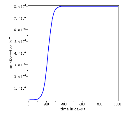 Figure 1
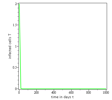 Figure 2
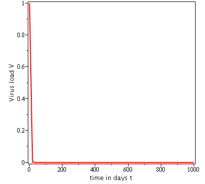 Figure 3
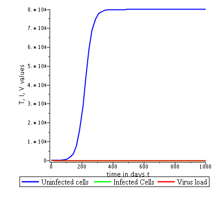 Figure 4
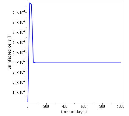 Figure 5
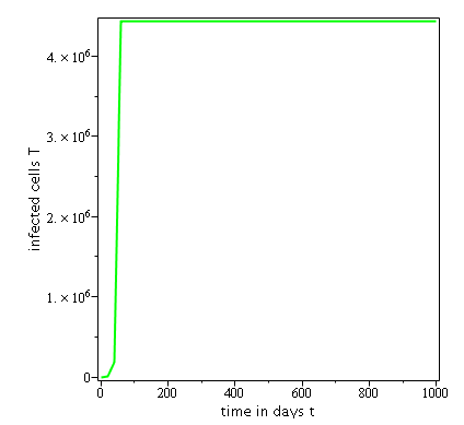 Figure 6
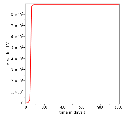 Figure 7
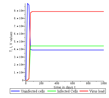 Figure 8
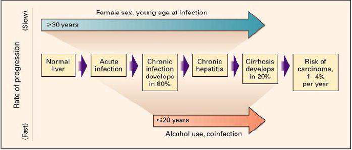 Figure 9
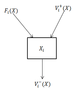 Figure 10
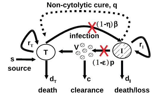 Figure 11
Peer Reviews
No public reviews on file for this paper yet. If you reviewed it on a platform where reviews are public (OpenReview, ICLR, NeurIPS, ICML), you can paste yours below so the community can read it here.
Videos
No videos yet. Explain this paper in a talk, walkthrough, or lecture? Add one.
Taxonomy
TopicsHepatitis C virus research · Mathematical and Theoretical Epidemiology and Ecology Models · Liver Disease Diagnosis and Treatment
Mathematical analysis of an extended
cellular model of the Hepatitis C Virus infection with non-cytolytic process
Alexis Nangue Email : Alexis Nangue : [email protected] University of Maroua, Higher Teacher’s Training College, Department of Mathematics, P.O.Box 55 Maroua, Cameroon
Cyprien Fokoue
University of Maroua, Faculty of Science, Department of Mathematics and Computer Science, Cameroon
Raoue Poumeni Now at : elsewhere University of Maroua, Higher Teacher’s Training College
Abstract
The aims of this work is to analyse of the global stability of the extended model of hepatitis C virus(HCV) infection with cellular proliferation, spontaneous cure and hepatocyte homeostasis. We first give general information about hepatitis C. Secondly, We prove the existence of local, maximal and global solutions of the model and establish some properties of this solution as positivity and asymptotic behaviour. Thirdly we show, by the construction of an appropriate Lyapunov function, that the uninfected equilibrium and the unique infected equilibrium of the model of HCV are globally asymptotically stable respectively when the threshold number and when . Finally, some numerical simulations are carried out using Maple software confirm these theoretical results.
keywords : HCV model; global solutions; non-cytolytic process; invariant set; Lyapunov functions; basic reproduction number; equilibrium points.
AMS Classification Subject 2010 : 92B99, 34D23, 92D25.
1 Introduction
Hepatitis C infection is a viral disease caused by Hepatitis C Virus (HCV) and being transmitted mainly by blood contact between an infected person and a healthy person. This virus that attacks the hepatocytes is one of the main causes of chronic diseases of the liver such as hepatocellular carcinoma, liver cancer and cirrhosis of the liver [1, 19]. According to the WHO [22] global report published in April 2017 on hepatitis, 200 to 300 million people worldwide are infected with HCV, and between 60 et 85 of these people develop chronic liver disease [22, 23]. Although there is considerable progress in the research for the fight against this infection whose virus was discovered in 1989 [1, 19] and which presents today six genotypes, ranked from 1 to 6 according to [19]. There is no vaccine for prevention yet [20, 22]. Concerning the treatment of HCV infection, since 2014, the new direct-acting antivirals combined with Interferon- and Ribavirin have been able to cure about 90 of cases of chronic infection, but leaves the chronic diseases whose infection has caused. HCV infection is therefore a major public health problem.
To understand the dynamics of HCV viral load and its infectious process, mathematical models have become an important and almost unavoidable tool[2, 16]. A model is a system of mathematical equations accounting for all known experimental data of the studied biological phenomenon. It makes it possible to better understand the phenomenon under consideration and to act on the system optimally. Until 2009, most research work on the modeling of viral dynamics of HCV only took into account the level of circulating virus in a human population, the case in vivo was almost ignored as it provides a better understanding of the pathogenesis of the virus as Harel Dahari et al [8] and Chong et al.[1].
Our goal is therefore to analyze the stability of an extended model of HCV infection in a patient with cell proliferation and spontaneous healing presented in [7, 20] to reveal significant information on pathogenesis and dynamics of this virus. The work is organized as follows : In section 1, first focuses on presentation of the epidemiological model and give some properties of its solutions, then we calculate the basic reproduction ratio , which is an indispensable element in the study and analysis of the models. is considered in the virus dynamics as a metric. We theoretically analyze the local stability and the global stability of the model by the linearization and Lyapounov’s functions respectively in section 2 and in section 3 we perform numerical simulations using biologically plausible parameter values in Table 1 to confirm the results obtained theoretically and we complete the work by an appendix.
2 A dynamical model of HCV infection and some
properties of the solutions of the differential system associated to the model
Mathematical modeling applies to the study of dynamics of infectious diseases seems to be one of the most interesting tool for designing control or eradication strategies of a disease like hepatitis C. It allows to test on computer different prevention scenarios and so help the decision-making in public health [14]. In the following sections, we will firstly present epidemiology and brief history of HCV dynamics, then describe the model itself, show the existence of solutions and establish some properties of these solutions and finally calculate the basic reproduction rate which is an important tool in epidemiology.
2.1 Epidemiology and history of HCV
2.1.1 HCV infection
HCV is a virus that attacks the cells of the liver and causes inflammation of the latter. This virus is present in the blood of an infected person and is, according to the WHO, mandatory declaration. It can live for about 5 to 7 weeks in the open air. In the long term, there may be very serious consequences such as cirrhosis and in some cases, liver cancer . This virus can remain for decades in the body without any apparent symptoms. According to [14, njou] six main genotypes HCV were identified whereas several subtypes play an important role in the severity of the disease and its response to treatment.
2.1.2 Epidemiology of HCV Infection
HCV infection is a major public health problem. Worldwide, the number of chronic HCV carriers is estimated at about 170 million, or of the world’s population, and the incidence is between 3 and 4 million infections per year according to the statistics published by the World Health Organization in 2014. The actual incidence is uncertain because the distinction between acute and chronic forms is difficult to make. HCV was only identified in 1989 with the advent of modern molecular cloning techniques.
In Cameroon, about 10,000 people die each year from hepatitis (A, B, C, D, …). The country is one of the 17 most affected worldwide, with a prevalence rate of about , that is 2.5 million people infected.
2.1.3 Natural history of HCV infection
According to WHO’s global report on hepatitis C published in April 2017 the first phase of HCV infection is said Acute: It can cause jaundice, but remains asymptomatic in the majority of cases (70 to 80 ), hence the risk of going unnoticed. It is estimated that 20 to 30 people infected will spontaneously clear the virus within the first six months after initial contact. If the virus persists, hepatitis progresses to chronicity. The liver reacts to HCV aggression by an inflammatory reaction, one of the components of which is fibrogenesis. Hepatic fibrosis is the main complication of chronic hepatitis C. Hepatitis C is likely to evolve at the chronic phase in about 25 of cases to cirrhosis within a period of 5 to 20 years. In case of cirrhosis, the incidence of hepatocellular carcinoma is high: on the order of 1 to 4 per year [14].(See figure 1).
In order to achieve our various goals, we first describe the model and its parameters.
2.2 Description of the HCV model with compartmental
diagram
There are two mathematical models of HCV dynamics : the original model or model of Newmann [17] and its extended models like that of Dahari [1, fashion]. Each model can be represented by a compartmental scheme. A compartmental scheme is a scheme for estimating the variation in the number of individuals in each compartment over time. Figure 2 is the schematic representation of the extended model, which we will study, of HCV with cellular proliferation and spontaneous healing designed by T. C. Reluga et al. [20]. This model expands the viral dynamics of the original model of infection and the disappearance of HCV by incorporating the proliferation and death density dependence. In addition to cell proliferation, the number of uninfected hepatocytes may increase through immigration or differentiation of hepatocyte precursors that develop into hepatocytes at a constitutive rate of or by spontaneous infected hepatocyte healing by a non-cytolytic process at the rate .
The model proposed by Dahari and coworkers [8, 4] expands on the standard HCV viral-dynamic model [17] of infection and clearance by incorporating density-dependent proliferation and death. Uninfected hepatocytes or noninfected hepatocytes, T, are infected at a rate per free virus per hepatocyte. Infected cells, I, produce free virus at rate per cell but also die with rate . Free virus is cleared at rate by immune and other degradation processes. Besides infection processes, hepatocyte numbers are influenced by homeostatic processes. Uninfected hepatocytes die at rate . Both infected and uninfected hepatocytes proliferate logistically with maximum rates and , respectively, as long as the total number of hepatocytes is less than . Besides proliferation, uninfected hepatocytes may increase in number through immigration or differentiation of hepatocyte precursors that develop into hepatocytes at constitutive rate , or by spontaneous cure of infected hepatocytes through a noncytolytic process at rate . Treatment with antiviral drugs reduces the infection rate by a fraction and the viral production rate by a fraction . It should be noted that and are parameters which values are non-negative and less than one.
The interpretations and biologically plausible value of other parameters are listed in following Table 1 , and a further comprehensive survey on the description of the model is given in [7, 6, 20].
Thus, the variation of healthy hepatocytes T is expressed by the following expression :
[TABLE]
The variation of infected hepatocytes I is expressed by the following expression:
[TABLE]
And the variation of the viral load V is expressed by the following expression :
[TABLE]
It follows that the dynamics of T, I and V is governed by the following differential system :
[TABLE]
System (4) is under the following initial conditions:
[TABLE]
Given the meanings of and , the term represents the mass action principle; is the rate of infection of healthy T cells by interaction with virus V.
For biological significance of the parameters, three assumptions are employed. (1) Due to the burden of supporting virus replication, infected cells may proliferate more slowly than uninfected cells, i.e. . (2) To have a physiologically realistic model, in an uninfected liver when is reached, liver size should no longer increase, i.e. . (3) Infected cells have a higher turnover rate than uninfected cells, i.e. . The interpretations and biologically plausible values of other parameters are listed in Table 1, and a further comprehensive survey on the description of (4) is given in [20]. Besides HCV infection, the similar model of (4) is also used to describe the dynamics of HBV or HIV infection, in which the full logistic terms mean the proliferation of uninfected/infected hepatocytes [3, 15, 5], or the mitotic transmission of uninfected/infected CD4+T.
The range of variation of each parameter is recorded in table 1 [20].
Table 1
Estimated parameter ranges for hepatitis C when modeled with system [20]. The , , and parameters are not independently identifiable, so common practice is to fix prior to fitting
[TABLE]
This table tells us in which interval varies each parameter of the model. For the study of stability and for simulations these ranges of values will have to be respected for a good decision-making.
2.3 Theorems of existence and some properties of solution
to the cauchy problem (4), (5)
2.3.1 Existence of local solutions
Theorem 2.1
Let . There exists and functions continuously differentiable such that is a solution of system (4) satisfying (5).
Proof**.** We will use the local Cauchy-Lipschitz theorem to proof this. Since the system of equations (4) is autonomous, it is enough to show that the function
[TABLE]
is locally Lipschitzian with:
[TABLE]
[TABLE]
[TABLE]
According to L. Perko [18], it is also enough to prove that is a class function.
The jacobian matrix of at is:
[TABLE]
i.e.
[TABLE]
Each component of this matrix being continuous, they are locally bounded for all . Therefore possesses continuous and bounded partial derivatives on any compact of . Thus is locally Lipschitzian with respect to . By the Cauchy-Lipschitz theorem, there is a local solution defined on This completes the proof of this theorem 2.1.
Remark 1
The function in the proof of theorem 2.1 is a class function so the system (4) has a unique maximal solution.
2.3.2 positivity of the system (4)
Theorem 2.2
*Let be a solution of the system (4) over an interval such that et .
If are positive, then , and are also positive for all .*
Proof**.** We are going to prove by contradiction. so suppose there is such that or or .
Let
Let also be the smallest of all in the interval such that and for a certain .
Then each of the equations of the system (4) can be written where is a non negative function and any function.
Thus,
[TABLE]
with
[TABLE]
and
[TABLE]
similarly;
[TABLE]
with
[TABLE]
and
[TABLE]
and
[TABLE]
with
[TABLE]
and
[TABLE]
Without loss the generality, suppose that .
As hypothesized, is positive on , it follows that
[TABLE]
from where
[TABLE]
Yet is a solution of (4). , , are class class functions. They are continuous on and therefore are bounded on . Thus is bounded on .
There exists a constant such that
[TABLE]
By integrating this previous expression on , we get
[TABLE]
Where
[TABLE]
This is a contradiction because .
Similarly, assuming that , as hypothesized, is positive on , it follows that
[TABLE]
Thus,
[TABLE]
Yet is a solution of system (4); , , are class functions. They are therefore continuous on and consequently are bounded on .
Therefore is bounded on .
Thus, there exists a constant such that
[TABLE]
Integrating, the last expression on , yields
[TABLE]
Therefore
[TABLE]
This is a contradiction because .
As far as that goes, assuming that .
By hypothesis, is positive on , we obtain i.e
[TABLE]
Hence integrating on we obtain
[TABLE]
This is a contraction.
Conclusion: , , are positive on .
It will now be shown, with the help of the continuation criterion the existence of global solutions of problem (4), (5).
2.3.3 Existence of global solutions
Theorem 2.3
The solutions of the Cauchy problem (4), (5), with positive initial data, exist globally in time in the future that is on .
Proof**.** To prove this it is enough to show that all variables are bounded on an arbitrary finite interval . Using the positivity, by the theorem 2.2, of the solutions it is enough to show that all variables are bounded above.
Taking the sum of equations (1), (2) shows that :
[TABLE]
and hence that . Thus and are bounded on any finite interval. The third equation, i.e.
[TABLE]
then shows that cannot grow faster than linearly and is also bounded on any finite interval. This completes the proof of this theorem.
2.3.4 Asymptotic behaviour
Theorem 2.4
For any positive solution of system (4), (5) we have :
[TABLE]
where
[TABLE]
Proof**.** Summing equations (1) and (2), we get:
[TABLE]
Let , , , and let us solve the following equation
[TABLE]
Coupled to equation (9) the initial condition :
[TABLE]
The resolution of the problem (9), (10) gives for all ,
[TABLE]
As for all , it follows that :
[TABLE]
i.e.
[TABLE]
Let
[TABLE]
we obtain :
[TABLE]
Therefore
[TABLE]
Since T and I are positive and , so it follows that and .
From (3), we have:
[TABLE]
According to Gronwall inequality,
[TABLE]
[TABLE]
[TABLE]
with
[TABLE]
This completes the proof of theorem 2.4.
Remark 2
It follows that all solutions of the system (4) are asymptotically uniformly bounded in compact subset defined by
[TABLE]
Remark 3
Theorem 2.4 shows that all solutions of model (4) in are ultimately bounded and according to theorem 2.2, that solutions with positive initial value conditions are positive, which indicates that model (4) is well-posed and biologically valid.
2.4 Basic reproduction ratio
One of the most important concerns about any infectious disease is its ability to invade a population. Many epidemiological models have a disease free equilibrium (DFE) at which the population remains in the absence of disease. These models usually have a threshold parameter, known as the basic reproduction number, , such that if , then the DFE is locally asymptotically stable, and the disease cannot invade the population, but if , then the DFE is unstable and invasion is always possible. In other words, we have the following definition :
Definition 2.5
[9]** The basic reproduction ratio or the basic reproduction number or basic reproductive ratio is defined as the expected number of secondary cases produced, in a completely susceptible population, by a typical infected individual during its entire period of infectiousness.
Determine in function of the parameters of the model allow us to guess the conditions under which the disease invade the population.
2.4.1 Determination of
the uninfected equilibrium or virus-free equilibrium or noninfected equilibrium
Proposition 2.6
The uninfected equilibrium point of the system (4) is given by
[TABLE]
where :
[TABLE]
Proof**.** When there is no viral infection, the uninfected hepatocytes dynamic is determined by :
[TABLE]
The quantity of the free-virus equilibrium point is solution of the equation .
Hence, let us solve the following equation :
[TABLE]
Its discriminant is given by :
[TABLE]
which yields :
[TABLE]
Thus, in the absence of viral infection, the amount of susceptible cells or uninfected hepatocytes attend to a positive constant level , which is :
[TABLE]
This completes the proof.
2.4.2 Computation of the basic reproduction number
We are going to use Van Den Driessche and Watmough method [9, 21] for calculating the basic reproduction ratio of the model (4).
Let us first present briefly the method.
Considering population whose population are grouped into homogeneous compartments where is the number of individuals in compartment . For clarity we sort the compartments , so that the first compartments correspond to infected individuals. The distinction between infected and uninfected compartments must be determined from the epidemiological interpretation of the model and cannot be deduced from the structure of the equations alone.
We define to be the set of all disease free states. That is :
[TABLE]
Let be the rate of appearance of new infections in compartment that is the infected individuals coming from other compartments and enter into .
be the rate of transfer of individuals into compartment by all other means (displacement, healing, aging).
be the rate of transfer of individuals out of compartment (mortality, change of statut).
It is assumed that each function is continuously differentiable at least twice in each variable.
Figure 3 below shows the variations of the number of individuals in compartment in a population.
The variation of the number of individuals in compartment is given by :
[TABLE]
where
[TABLE]
Due to the nature of the epidemiological model, we have the following properties :
If then , and .
Since each function represents a directed transfer of individuals. 2.
If then .
Indeed, If a compartment is empty, then there can be no transfer of individuals out of the compartment by death, infection, nor any other means : it is the essential property of a compartmental model. 3.
Pour , .
In fact, the compartments with an index greater than are ”uninfected”. By definition, it can not appear in these compartments infected individual. 4.
Si alors et pour , .
Indeed, to ensure that the disease free subspace is invariant, we assume that if the population is free of disease then the population will remain free of disease. That is, there is no (density independent) immigration of infectives. This is Lavoisier’s principle. There is no spontaneous generation.
Let and .
Let also the uninfected equilibrium point of the corresponding model.
Let and denote the jacobian matrices of F and V respectively at the point .
It follows that is a positive matrix and a Metzler matrix (matrix whose the extra diagonal terms are greater or equal than zero ). Thus we have the following equivalent definition of :
Definition 2.7
[TABLE]
where represents the spectral radius. i.e
[TABLE]
with
[TABLE]
where is the spectrum of , i.e. the set of eigenvalues associated to a matrix
2.4.3 Expression of the basic reproduction number
associated to the system (4)
Proposition 2.8
The expression of the basic reproduction number associated to the system (4) is given by :
[TABLE]
where
[TABLE]
Proof**.** Concerning the model (4) that we study here, the system of infected states is the following :
\left\{\begin{array}[]{lcr}\dfrac{dI}{dt}=r_{I}I\left(1-\dfrac{T+I}{T_{max}}\right)+(1-\eta)\beta VT-d_{I}I-qI\\ \\ \dfrac{dV}{dt}=(1-\varepsilon)pI-cV\end{array}\right.
The expression of the quantities , , , and are given by:
, ,
, ,
From those quantities, we obtain:
= .
Let . It follows that :
[TABLE]
Therefore :
[TABLE]
which completes the proof of the proposition.
Remark 4
* denotes the overall effectiveness rate of the drug .*
Remark 5
Henceforth, we will let and .
At the end of this section, we note that HCV is a major health problem in the world and particularly in Cameroon where it affects almost 13% of population.
For the model (4) which is the subject of our work, we have shown the existence of the global solution and establish some properties like positivity. The calculation of has been done.
In the next section, we will determine the infected equilibrium point and establish the conditions on for which stability of the model occurs.
3 Stability analysis of the model
In this section, we study the local stability and global stability of the equilibrium points and we present some numerical simulations of the theoretical results obtained. Specifically, we prove by Lyapunov’s theory that the uninfected equilibrium point is globally asymptotically stable if and the infected equilibrium point is globally asymptotically stable when it exists.
Before that we establish a number of essential preliminary results for the next steps
3.1 Invariant set of the model
Theorem 3.1
Let and be a maximal solution of the Cauchy problem (4), (5) (). If and then the set :
[TABLE]
where :
[TABLE]
is a positively invariant set by system (4).
Proof**.** Let . We shall show that :
- (i)
If then for all , . 2. (ii)
If then for all , .
- i)
Let us show i) by contradiction.
Let us suppose that there exists such that we have
[TABLE]
Let
If then since
[TABLE]
when . In addition, according to equations (1) and (2) of system (4), we have
[TABLE]
Recall that
[TABLE]
It follows that :
[TABLE]
Hence, there exists such that for all , which is a contradiction. Therefore for all , . 2. ii)
Let us show ii) by contradiction.
Let us suppose that there exists such that and
[TABLE]
Let .
Since , since:
[TABLE]
with when .
Equation (3) yields :
[TABLE]
yet
[TABLE]
consequently
[TABLE]
Thus, there exists such that for all , which is a contradiction. Therefore for all , Which completes the proof of Theorem 3.1.
3.2 Existence of the infected equilibrium point
When it exists, the infected equilibrium point is given by: where , and are positive constants that we are going to determine.
Lemma 3.2
* exists if and only if*
[TABLE]
Proof**.** Let us consider the following system of algebraic equations :
[TABLE]
(15) yields :
[TABLE]
Reporting (16) in (14), we have :
[TABLE]
Hence
[TABLE]
i.e
[TABLE]
It follows that :
[TABLE]
Let
[TABLE]
Reporting (16) and (17) in (13) leads to :
[TABLE]
i.e.
[TABLE]
Thus ,
[TABLE]
It follows that,
[TABLE]
Let
[TABLE]
we have :
[TABLE]
with :
[TABLE]
Since , the polynomial (19) has a unique positive root if and only if :
[TABLE]
This completes the proof of Lemma 3.2.
Suppose that , we have the following results :
Lemma 3.3
If , then :
- i)
* if and only if * 2. ii)
* if and only if .*
Remark 6
* of Lemma 3.3 is the solution of equation i.e*
[TABLE]
Proposition 3.4
Suppose that .
- •
If , then . Hence, system (4) admits no infected equilibrium point.
- •
If then :
- i)
system (4) admits no infected equilibrium point when . 2. ii)
system (4) admits a unique infected equilibrium point when .
Lemma 3.5
.
Proof**.** Since is the root of equation (18), we have :
[TABLE]
Lemma 3.6
* if and only if .*
Proof**.** We have :
[TABLE]
Since , the equivalence of the Lemma 3.6 allows us to write .
The following proposition establishes the link between and the existence of the equilibrium point when .
Proposition 3.7
Suppose that exists, and , then :
- i)
* if .* 2. ii)
* if .*
Proof**.** Recall that if and only if and if and only if
Using the expression of given in (19) we have :
[TABLE]
Thus
[TABLE]
Yet
[TABLE]
and
[TABLE]
Hence,
[TABLE]
Since and , we get :
[TABLE]
and
[TABLE]
This completes the proof of Proposition 3.7.
Suppose now , then equation (19) admits a unique positive solution and we have the following results:
Lemma 3.8
Suppose that , then :
- •
* if and only if .*
- •
* if and only if .*
Remark 7
* of lemma 3.8is the solution of equation , i.e*
[TABLE]
Proposition 3.9
- i)
If , then and the system (4) admits in this case a unique infected equilibrium point . 2. ii)
If , alors :
- •
the system (4) not admits an infected equilibrium point when .
- •
the system (4) admits a unique infected equilibrium point when .
We state the following two lemmas whose the proofs are analogous of those of lemma 3.5 and lemma 3.6 respectively. These lemmas will help us to complete the conditions of existence of the infected equilibrium point
Lemma 3.10
**
Lemma 3.11
* if and only if .*
Proposition 3.12
*Suppose that : and .
Then if , and if .*
Proof**.** Recall that if and only if and if and only if From the expression of given by (19) we have :
[TABLE]
Thus :
[TABLE]
yet
[TABLE]
[TABLE]
[TABLE]
Hence :
[TABLE]
Since d_{T}-r_{T}\Big{(}1-\frac{T^{0}}{T_{max}}\Big{)}>0 and , we get :
- •
if .
- •
if .
This completes the the proof.
The conditions of existence of an infected equilibrium point have been established, we are going in the following subsection give its expression.
3.3 Expression of the equilibrium points
3.3.1 Uninfected equilibrium point
By the proposition 2.6, the uninfected equilibrium point is given by where
[TABLE]
3.3.2 Infected equilibrium point
Lemma 3.13
When it exists, is defined by :
[TABLE]
where :
[TABLE]
[TABLE]
[TABLE]
and
[TABLE]
Proof**.** When exists, it will be a positive solution of the equation of second degree :
[TABLE]
with :
[TABLE]
Let
[TABLE]
then (20) becomes :
[TABLE]
Let also :
[TABLE]
then (20) becomes :
[TABLE]
Let :
[TABLE]
[TABLE]
[TABLE]
hence the previous equation yields :
[TABLE]
Its discriminant is:
[TABLE]
i.e.
[TABLE]
Hence
[TABLE]
[TABLE]
Where
[TABLE]
We have :
[TABLE]
with
[TABLE]
It follows that :
[TABLE]
The combination of the proposition 3.4, proposition 3.12 and the lemma 3.13 leads to the following theorem :
Theorem 3.14
The model (4) admits a unique infected equilibrium if and only if , where
[TABLE]
where where :
[TABLE]
[TABLE]
[TABLE]
and
[TABLE]
When the unique equilibrium is the uninfected equilibrium point or the infection-free steady state .
3.4 Local stability analysis of the
model 1 at the equilibrium points
For the study of local stability of the model (4) at the equilibrium points, let us consider once more the functions , et given by (6), (7) and (6) respectively.
3.4.1 Case of the uninfected equilibrium point
or infection-free steady state
Theorem 3.15
The infection-free steady state of model (4) is locally asymptotically stable if and unstable if .
Proof**.** The Jacobian matrix of the system (4) at is as the following :
[TABLE]
i.e.
[TABLE]
Since
[TABLE]
it follows that :
[TABLE]
Now let us show that the eigenvalues of the matrix have negative real part if and only if .
Considering the expression of , is a negative eigenvalue of the matrix . Now let us consider the sub-matrix defined by :
[TABLE]
The trace of is :
[TABLE]
and the determinant of is:
[TABLE]
The system (4) est locally asymptotically stable at if and only if
[TABLE]
and
[TABLE]
i.e.
[TABLE]
Therefore the model (4), is locally asymptotically stable at when and unstable when This completes the proof of theorem 3.15
3.4.2 Case of infected equilibrium point
We start this subsection by two preliminary lemmas.
Lemma 3.16
The Jacobian matrix , of lemma 3.16 , of system (4) at is given by :
[TABLE]
Proof**.** See the Appendice for the proof.
Lemma 3.17
The characteristic equation of the Jacobian matrix of the system (4) at is given by the following cubic equation :
[TABLE]
where :
[TABLE]
Proof**.** See the appendice for the proof of lemma 3.17.
Now let :
[TABLE]
By Routh-Hurwitz criteria[16], we have the following results.
Theorem 3.18
For model (4), when is valid, the unique endemic equilibrium is locally asymptotically stable if and unstable if .
Especially, we have :
Corollary 3.19
The infected steady state during the therapy of the model (4) is locally asymptotically stable if and unstable if .
Proof**.** Since , , it remains to show that .
[TABLE]
[TABLE]
[TABLE]
where,
[TABLE]
and
[TABLE]
Since , it remains to show that .
From (1) we have :
[TABLE]
yet
[TABLE]
hence,
[TABLE]
Thus,
[TABLE]
it follows that ;
[TABLE]
Reporting this previous expression in (25) yields :
[TABLE]
Taking especially and , we obtain : . Thus,
[TABLE]
and , therefore the system (4) is locally asymptotically stable at This completes the proof of Corollary 3.19.
3.5 Global stability analysis of the
system at equilibrium points
The global stability analysis of a dynamical system is usually a very complex problem. One of the most efficient methods to solve this problem is Lyapunov’s theory. To build the functions of Lyapunov we will follow the method proposed by A. Korobeinikov [11, 12, 13].
3.5.1 Case of infection-free steady state
Theorem 3.20
The infection-free steady state of the model (4) is globally asymptotically stable if the basic reproduction number and unstable if .
Proof**.** Consider the Lyapunov function :
[TABLE]
is defined, continuous and positive definite for all , , . Also, the global minimum occurs at the infection free equilibrium . Further, function , along the solutions of system (1), satisfies :
[TABLE]
[TABLE]
yet
[TABLE]
hence, further collecting terms, we have :
[TABLE]
[TABLE]
[TABLE]
[TABLE]
[TABLE]
Furthermore ,
[TABLE]
hence
[TABLE]
Since and , we have
and if and only if and simultaneously.
Therefore, the largest compact invariant subset of the set
[TABLE]
is the singleton . By the Lasalle invariance principle[10], the infection-free equilibrium is globally asymptotically stable if . We have seen previously that if , at least one of the eigenvalues of the Jacobian matrix evaluated at has a positive real part. Therefore, the infection-free equilibrium is unstable when . This completes the proof of the theorem.
Remark 8
The Lyapunov function defined in the proof of theorem 3.20 has been obtained following the general giving by Korobonikov [12, 13, 11] for the dynamic virus fondamental model.
3.5.2 Case of infected equilibrium point
We recall :
Remark 9
According to (13, 14, 15) the infected equilibrium point verify :
[TABLE]
[TABLE]
[TABLE]
Theorem 3.21
*Suppose that , and .
Then the infected steady state during therapy of model (4) is globally asymptotically stable as soon as it exists.*
Proof**.** Consider the Lyapunov function defined by :
[TABLE]
Let us show that and if and only if , , simultaneously.
The time derivative of along the trajectories of system (4) is :
[TABLE]
[TABLE]
[TABLE]
Collecting terms, and canceling identical terms with opposite signs, yields :
[TABLE]
Reporting equalities of remark 9 into (26), we have :
[TABLE]
[TABLE]
[TABLE]
[TABLE]
[TABLE]
[TABLE]
Note that
[TABLE]
and
[TABLE]
According to (13),
[TABLE]
furthermore,
[TABLE]
hence,
[TABLE]
By hypothesis, this leads to :
[TABLE]
[TABLE]
[TABLE]
Yet
[TABLE]
since the geometric mean is less than or equal to the arithmetic mean.
It should be noted that and holds if and only if take the steady states values . Therefore the infected equilibrium point is globally asymptotically stable. This completes the proof of this theorem.
3.6 Some numerical simulations
Some numerical simulations have been done in the case to confirm theoretical result obtain on global stability for the uninfected equilibrium.
The following curves, obtained using the Maple software, show the real-time evolution of uninfected hepatocytes, infected hepatocytes and viral load. The values of the parameters are taken in the parameter range defined by the table (2.2) and the initial conditions are , and .
3.6.1 Evolution in time of uninfected cells,
infected cells and viral load when
. Parameters values : , , , , , , , , , , , . These parameters values yields : and .
3.6.2 Evolution in time of uninfected cells,
infected cells and viral load when .
Parameters values: , , , , , , , , , , , . These parameters values yields: et .
In short, in this section, it was a question to study the global stability of the model (4). We have established that the model (4) is globally asymptotically stable at equilibrium points and when and unstable when . the numerical simulations has been carried out using the Maple software confirming theoretical results.
Acknowledgement(s)
I am grateful to Professor Alan Rendall for valuable and tremendous discussions. I wish to thank him for introducing me to Mathematical Biology and to its relationship with Mathematical Analysis. I also thank the Higher Teacher’s Training College of the University of Maroua were this paper were initiated.
Conclusion and discussions
Having reached the end of our work, it emerges from all the investigations presented that hepatitis C is a major health problem in the world and especially in Cameroon. To understand the dynamics of HCV and its infectious processes, mathematical models are present as an important and unavoidable tool. Global stability analysis has been done, by the technique of Lyapunov, to the model of HCV infection with proliferation cell and spontaneous healing, for revealing significant information for making good decision for the fighting against hepatitis C. We first show the existence of the global solution to the Cauchy problem (4), (5); then we have calculated the basic reproduction ratio . We finally show that the only infected equilibrium point for the model is globally asymptotically stable when and unstable when under others hypotheses. Furthermore uninfected equilibrium point for the model is globally asymptotically stable when and unstable when . These theoretical results have been confirmed by numerical simulations done using the software Maple. Given the results obtained, this work is the beginning point of very interesting other future investigations.
We plan to extend our analysis by focusing on more realistic models such as:
models with delay which involve delay ordinary differential equations; 2. 2.
models taking into account space which involve Partial differential equations; 3. 3.
models taking into account random phenomena which evolve stochastic differential equations.
We also plan to focus on others methods of studying global stability like the geometric method that can provides results with less hypotheses on model (4).
4 Appendices
Appendix A Proof lemma 3.16
Proof**.** The Jacobian matrix of the system (4) at is given by :
[TABLE]
Let us determine the coefficients of that Jacobian matrix .
[TABLE]
Yet
[TABLE]
[TABLE]
and
[TABLE]
hence ,
[TABLE]
[TABLE]
[TABLE]
[TABLE]
[TABLE]
[TABLE]
[TABLE]
[TABLE]
[TABLE]
[TABLE]
[TABLE]
[TABLE]
[TABLE]
[TABLE]
[TABLE]
Therefore, J(E^{\ast})=\left(\begin{array}[]{ccc}-\frac{s}{T^{\ast}}-\frac{r_{T}T^{\ast}}{T_{max}}-q\frac{I^{\ast}}{T^{\ast}}&-\frac{r_{T}T^{\ast}}{T_{max}}+q&-(1-q)\beta T^{\ast}\\ &&\\ \\ -\frac{r_{I}I^{\ast}}{T_{max}}+(1-\eta)\beta V^{\ast}&-\frac{r_{I}I^{\ast}}{T_{max}}-\frac{(1-\eta)\beta V^{\ast}T^{\ast}}{I^{\ast}}&(1-\eta)\beta T^{\ast}\\ \\ 0&(1-\varepsilon)p&-C\\ \\ \end{array}\right).
This completes the proof of the lemma 3.16.
Appendix B Proof of lemma 3.17
Proof**.** The characteristic equation is given by , i.e.
=0.
With
[TABLE]
it follows that :
[TABLE]
if and only if \left[-\frac{s}{T^{\ast}}-\frac{r_{T}T^{\ast}}{T_{max}}-\frac{qT_{max}}{T^{\ast}}\Big{(}-\frac{\delta}{r_{I}}+1\Big{)}-q\Big{(}\frac{A}{r_{I}}-1\Big{)}-\lambda\right]\Big{[}(c+\lambda)\Big{(}\frac{r_{I}I^{\ast}}{T_{max}}+\frac{(1-\eta)\beta V^{\ast}T^{\ast}}{I^{\ast}}+\lambda\Big{)}\\ \\ -(1-\varepsilon)p(1-\eta)\beta T^{\ast}\Big{]}\\ \\ +\left[\frac{r_{I}I^{\ast}}{T_{max}}+(1-\eta)\beta V^{\ast}\right]\Bigl{[}(c+\lambda)\Big{(}\frac{r_{T}T^{\ast}}{T_{max}}-q\Big{)}++(1-\varepsilon)p(1-\eta)\beta T^{\ast}\Bigr{]}=0, i.e.
[TABLE]
[TABLE]
i.e
\lambda^{2}\Big{[}-\frac{s}{T^{\ast}}-\frac{r_{T}T^{\ast}}{T_{max}}-\frac{qT_{max}}{T^{\ast}}\Big{(}-\frac{\delta}{r_{I}}+1\Big{)}-q\Big{(}\frac{A}{r_{I}}-1\Big{)}\Big{]}+\lambda\Big{[}\Big{(}c+\frac{r_{I}I^{\ast}+AT^{\ast}}{T_{max}}\Big{)}-\frac{s}{T^{\ast}}\\ \\ -\frac{r_{T}T^{\ast}}{T_{max}}-\frac{qT_{max}}{T^{\ast}}\Big{(}-\frac{\delta}{r_{I}}+1\Big{)}-q\Big{(}\frac{A}{r_{I}}-1)\Big{)}\Big{]}+\frac{cr_{I}I^{\ast}}{T_{max}}\Big{[}-\frac{s}{T^{\ast}}-\frac{r_{T}T^{\ast}}{T_{max}}-\frac{qT_{max}}{T^{\ast}}\Big{(}-\frac{\delta}{r_{I}}+1\Big{)}\\ \\ -q\Big{(}\frac{A}{r_{I}}-1\Big{)}\Big{]}-\lambda^{3}-\lambda^{2}\Big{(}c+\frac{r_{I}I^{\ast}+AT^{\ast}}{T_{max}}\Big{)}-\lambda\frac{cr_{T}I^{\ast}}{T_{max}}+\lambda\Big{(}\frac{r_{T}T^{\ast}}{T_{max}}-q\Big{)}\Big{(}\frac{r_{I}I^{\ast}-AI^{\ast}}{T_{max}}\Big{)}\\ \\ +\frac{r_{I}I^{\ast}-AI^{\ast}}{T_{max}}\Big{[}\frac{cr_{T}T^{\ast}+AcT^{\ast}}{T_{max}}-qc\Big{]}=0.
By developing the different factors in the previous equation, we get :
\lambda^{3}+\lambda^{2}\Big{[}\frac{s}{T^{\ast}}+\frac{r_{T}T^{\ast}}{T_{max}}+\frac{qT_{max}}{T^{\ast}}\Big{(}-\frac{\delta}{r_{I}}+1\Big{)}+q\Big{(}\frac{A}{r_{I}}-1\Big{)}+c+\frac{r_{I}I^{\ast}+AT^{\ast}}{T_{max}}\Big{]}\\ \\ +\lambda\Big{[}(c+\frac{r_{I}I^{\ast}+AT^{\ast}}{T_{max}})(\frac{s}{T^{\ast}}+\frac{r_{T}T^{\ast}}{T_{max}}+\frac{qT_{max}}{T^{\ast}}\Big{(}-\frac{\delta}{r_{I}}+1\Big{)}+q\Big{(}\frac{A}{r_{I}}-1)\Big{)}+\frac{cr_{I}I^{\ast}}{T_{max}}+\Big{(}q-\frac{r_{T}T^{\ast}}{T_{max}}\Big{)}\Big{(}\frac{r_{I}I^{\ast}-AI^{\ast}}{T_{max}}\Big{)}\Big{]}\\ \\ +\Big{[}\frac{cr_{I}I^{\ast}}{T_{max}}\Big{(}\frac{s}{T^{\ast}}+\frac{r_{T}T^{\ast}}{T_{max}}+\frac{qT_{max}}{T^{\ast}}\Big{(}-\frac{\delta}{r_{I}}+1\Big{)}q\Big{(}\frac{A}{r_{I}}-1\Big{)}\Big{)}+\frac{r_{I}I^{\ast}-AI^{\ast}}{T_{max}}\Big{(}qc-\frac{cr_{T}T^{\ast}+AcT^{\ast}}{T_{max}}\Big{)}\Big{]}=0.
Let:
[TABLE]
we have:
[TABLE]
Let also :
[TABLE]
we have :
[TABLE]
[TABLE]
[TABLE]
[TABLE]
Let once more :
[TABLE]
We get :
[TABLE]
[TABLE]
Therefore,
[TABLE]
with
[TABLE]
[TABLE]
and
[TABLE]
This completes the proof of the lemma 3.17.
The reference list from the paper itself. Each links out to its DOI / PubMed record.
- 1[1] M. S. F. Chong, L.S.M.Crossley and Madzvamuse, The stability analyses of the mathematical models of hepatitis C virus infection . Modern Applied Science, 9 (3). pp. 250-271. ISSN 1913-1844, Article (Published Version) Anotida (2015), 23 pages. http://sro.sussex.ac.uk/52312/
- 2[2] Y. Cherruault, Biomath matiques , Presses Universitaire de France, 1983, 108, boulevard Saint-Germain, 75006 Paris 2014, 132 pages.
- 3[3] S. M. Ciupe, R. M. Ribeiro, P. W. Nelson and A. S. Perelson, Modeling the mechanisms of acute hepatitis B virus infection , J. Theor. Biol. 247 (2007) 23 35.
- 4[4] H. Dahari, R. M. Ribeiro, and A. S. Perelson, Triphasic decline of HCV RNA during antiviral therapy, Hepatology , 46 (2007), pp. 16 21.
- 5[5] H. Dahari, E. Shudo, R. M. Ribeiro, and A. S. Perelson, Modeling complex decay profiles of hepatitis B virus during antiviral therapy, Hepatology , to appear (DOI: 10.1002/hep.22586).
- 6[6] H. Dahari, J. E. Layden-Almer, E. Kallwitz, R. M. Ribeiro, S. J. Cotler, T. J. Layden and A. S. Perelson, A mathematical model of hepatitis C virus dynamics in patients with high baseline viral loads or advanced liver disease , Gastroenterology 136 (2009) 1402 1409.
- 7[7] H. Dahari, M. Major, X.Zhang, K.Mihalik, C. M. Rice, A. S. Perelson, S. M. Feinstone and A.U.Neumann Mathematical Modeling of Primary Hepatitis C Infection: Noncytolytic Clearance and Early Blockage of Virion Production , Gastroenterology 128 2005:1056 1066.
- 8[8] H. Daharia, A. Loa, R. M. Ribeiroa, A. S. Perelson; Modeling hepatitis C virus dynamics: Liver regeneration and critical drug efficacy . Journal of Theoretical Biology 247 (2007) 371 381, 2007, P.371-381. www.sciencedirect.com.