Consistency of Gauged Two Higgs Doublet Model: Gauge Sector
Cheng-Tse Huang, Raymundo Ramos, Van Que Tran, Yue-Lin Sming Tsai and, Tzu-Chiang Yuan

TL;DR
This paper analyzes constraints on the gauge sector parameters of the gauged two Higgs doublet model using data from LEP, LHC, and projected CEPC sensitivities, clarifying the role of the Stueckelberg mass.
Contribution
It provides the first comprehensive analysis of gauge sector constraints in the gauged two Higgs doublet model using current and future collider data.
Findings
Constraints on new gauge parameters from LEP and LHC data
Projected sensitivities of CEPC on model parameters
Clarification on the zero Stueckelberg mass for hypercharge
Abstract
We study the constraints on the new parameters in the gauge sector of gauged two Higgs doublet model using the electroweak precision test data collected from the Large Electron Positron Collider (LEP) at and off the Z-pole as well as the current Drell-Yan and high-mass dilepton resonance data from the Large Hadron Collider (LHC). Impacts on the new parameters by the projected sensitivities of various electroweak observables at the Circular Electron Positron Collider (CEPC) proposed to be built in China are also discussed. We also clarify why the St\"{u}eckelberg mass for the hypercharge is set to be zero in the model by showing that it would otherwise lead to the violation of the standard charge assignments for the elementary quarks and leptons.
Click any figure to enlarge with its caption.
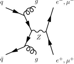 Figure 1
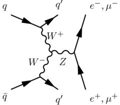 Figure 2
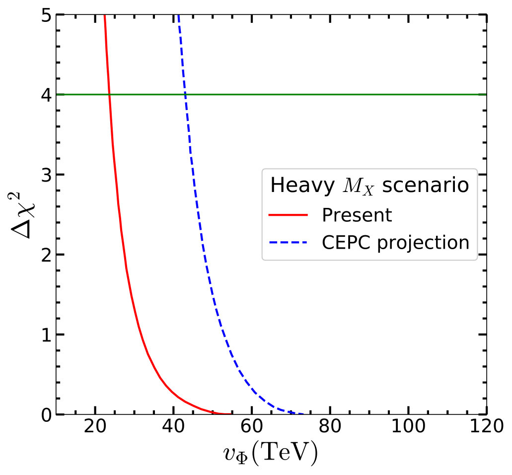 Figure 3
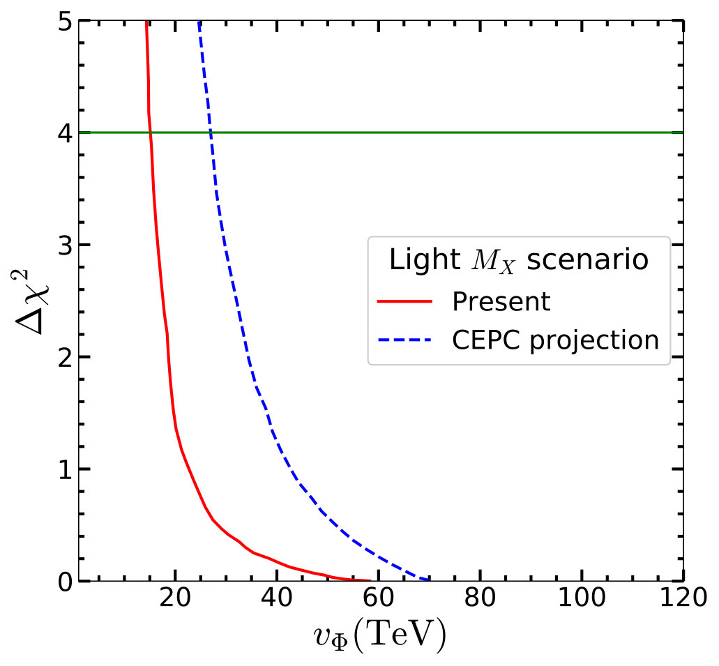 Figure 4
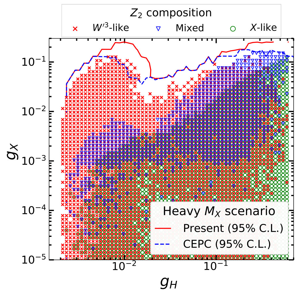 Figure 5
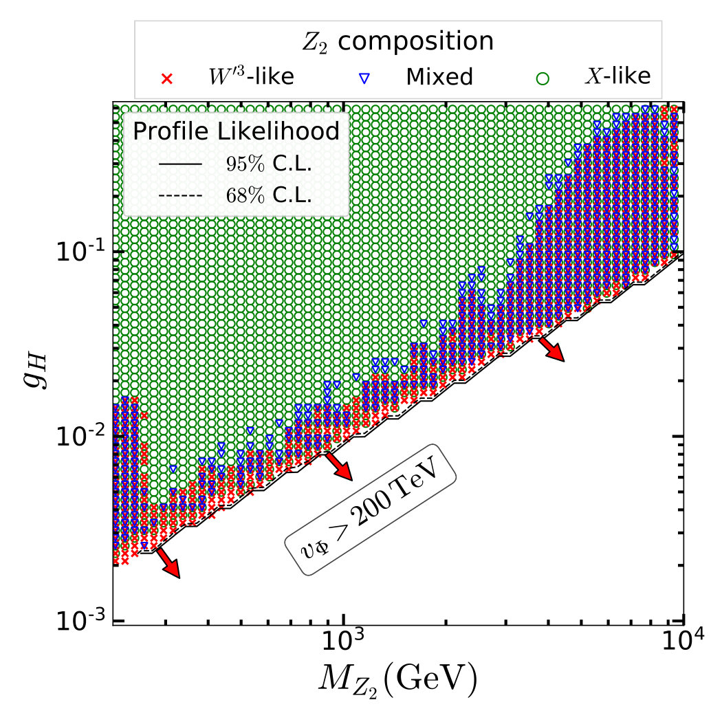 Figure 6
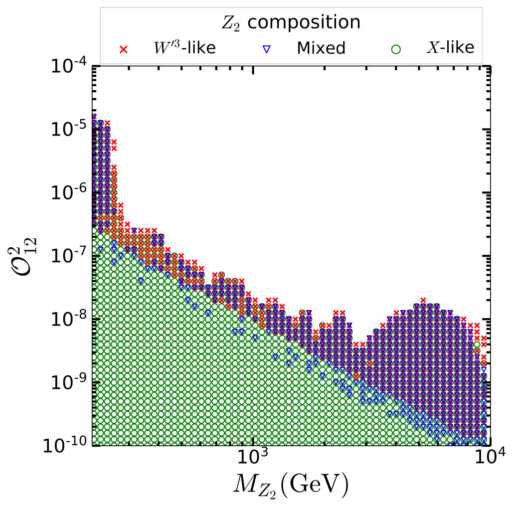 Figure 7
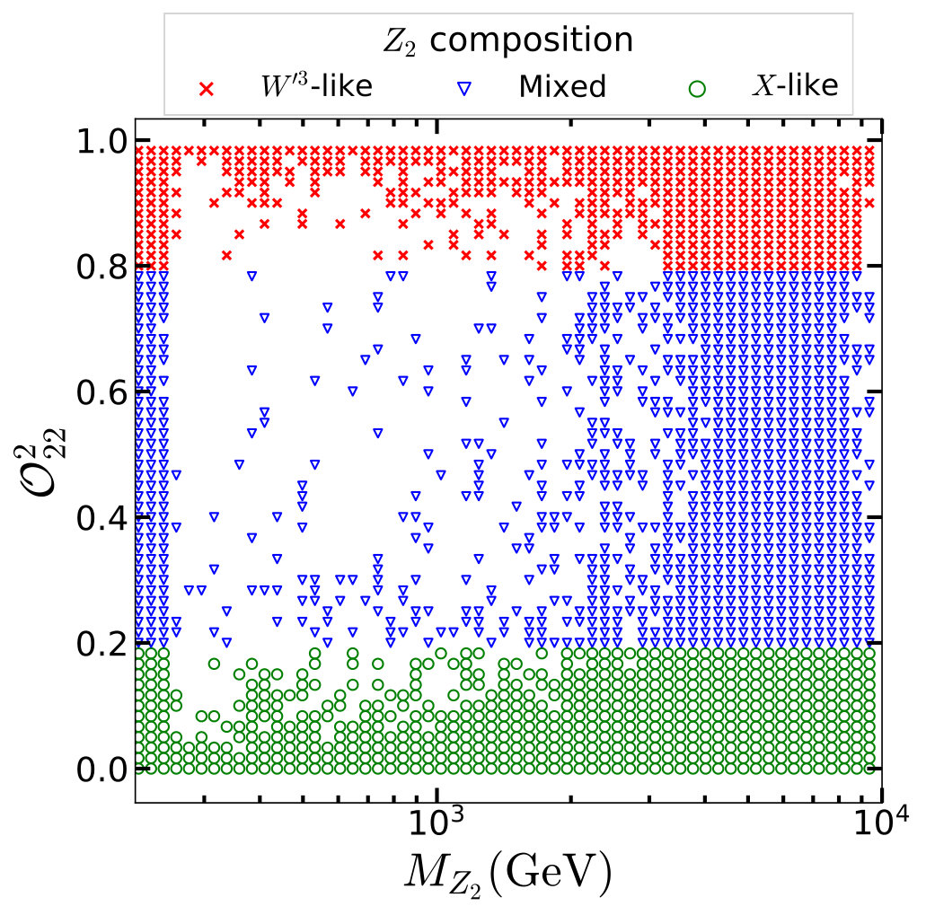 Figure 8
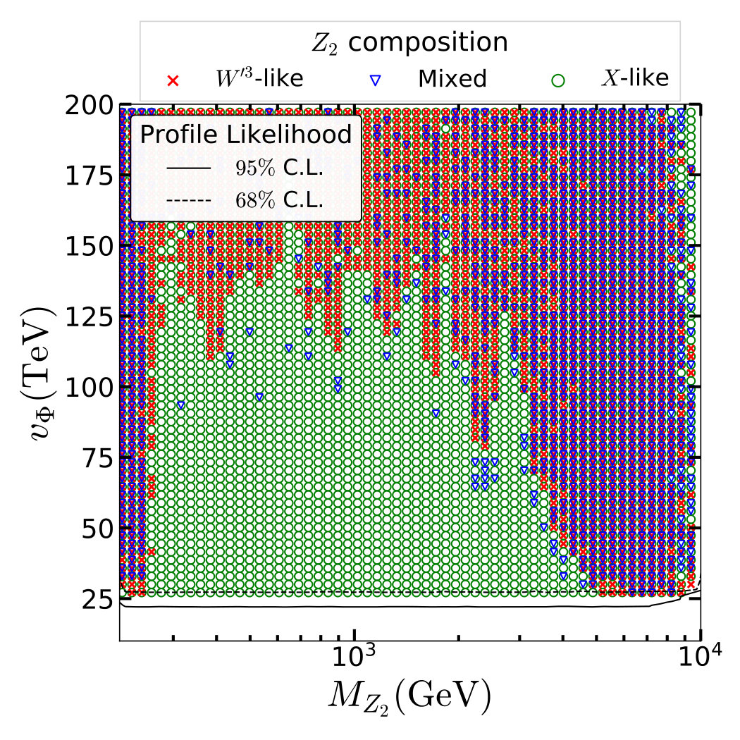 Figure 9
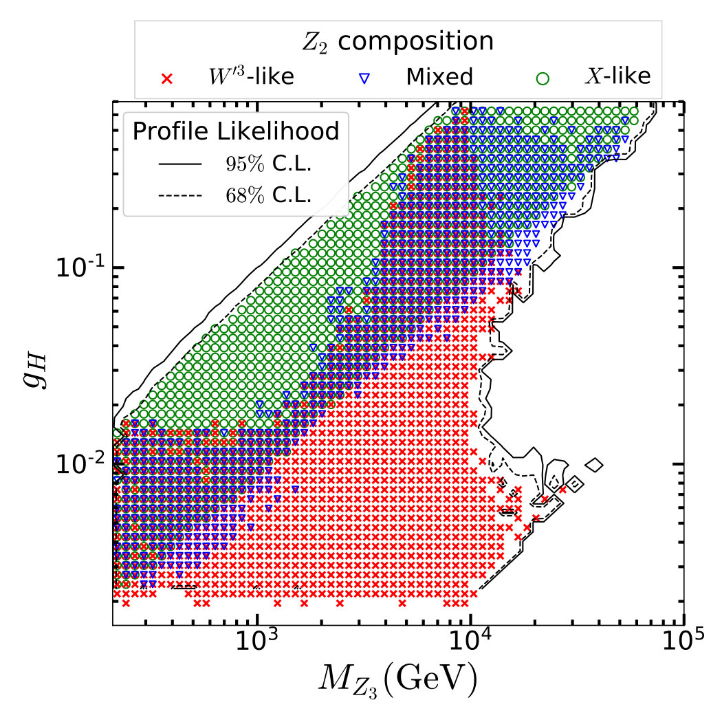 Figure 10
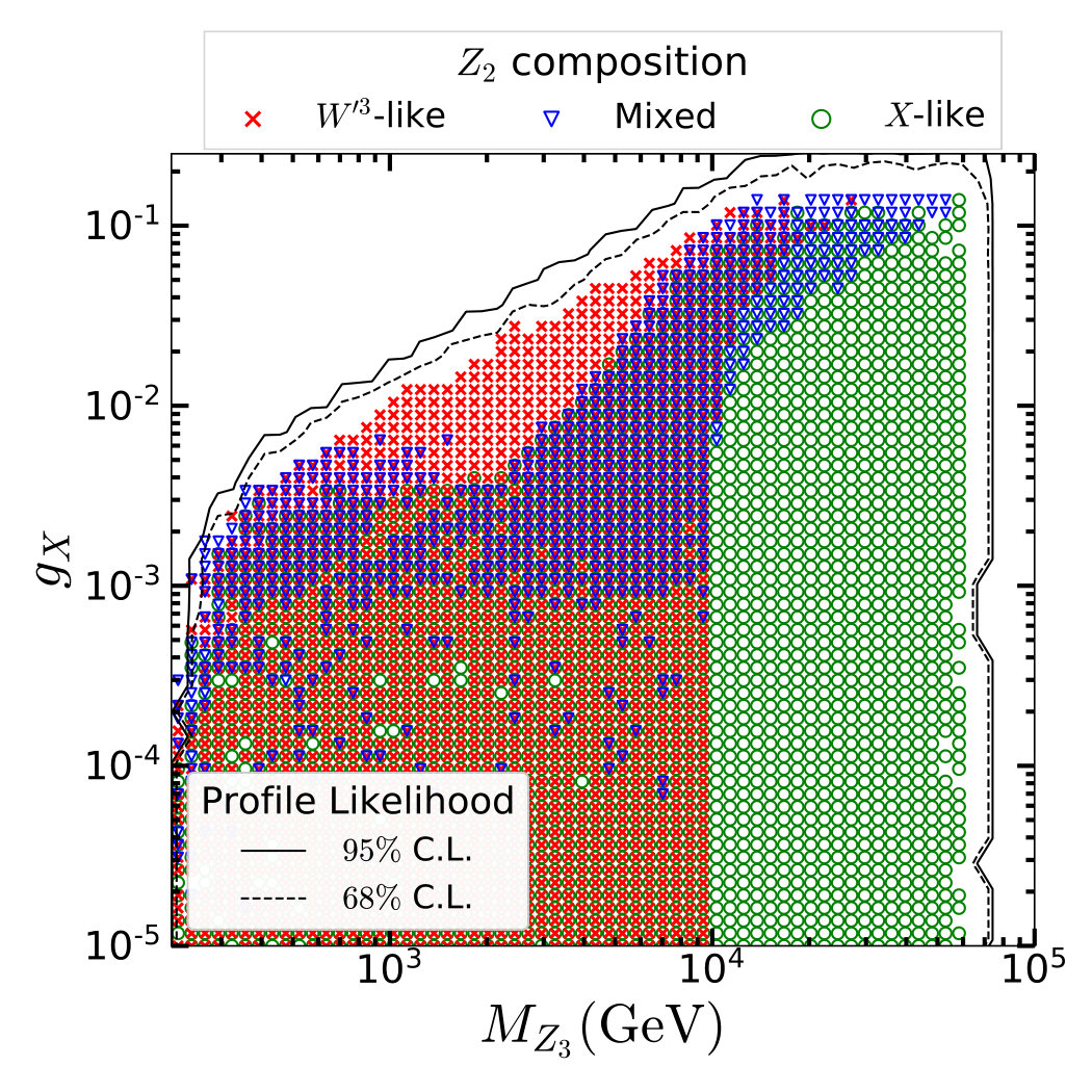 Figure 11
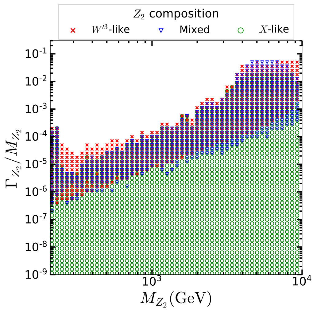 Figure 12
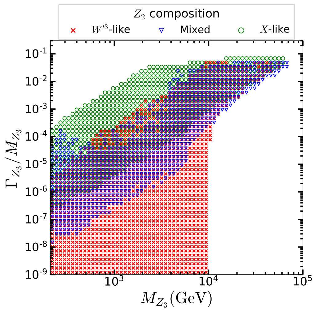 Figure 13
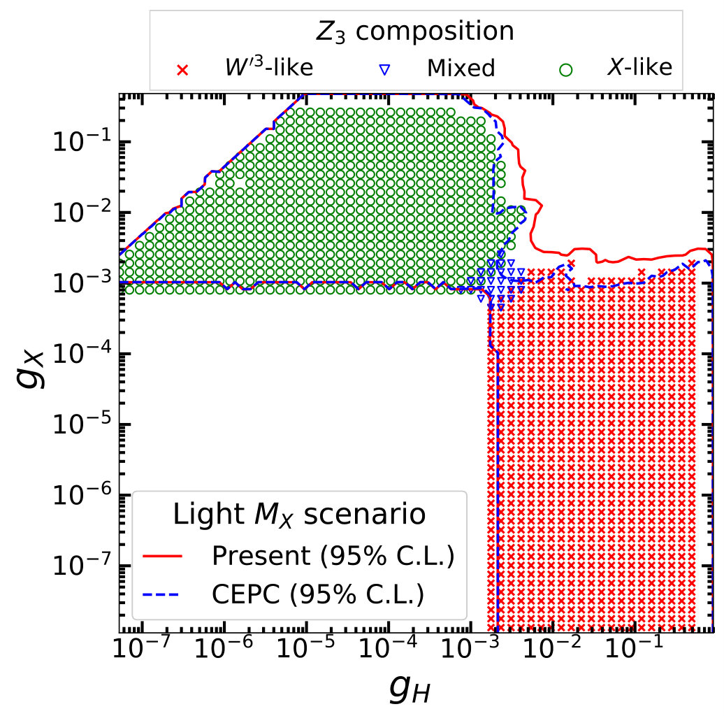 Figure 14
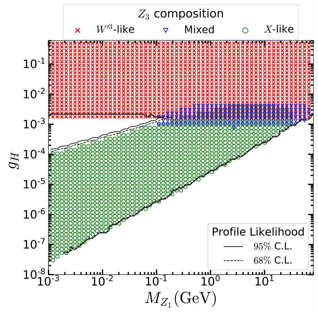 Figure 15
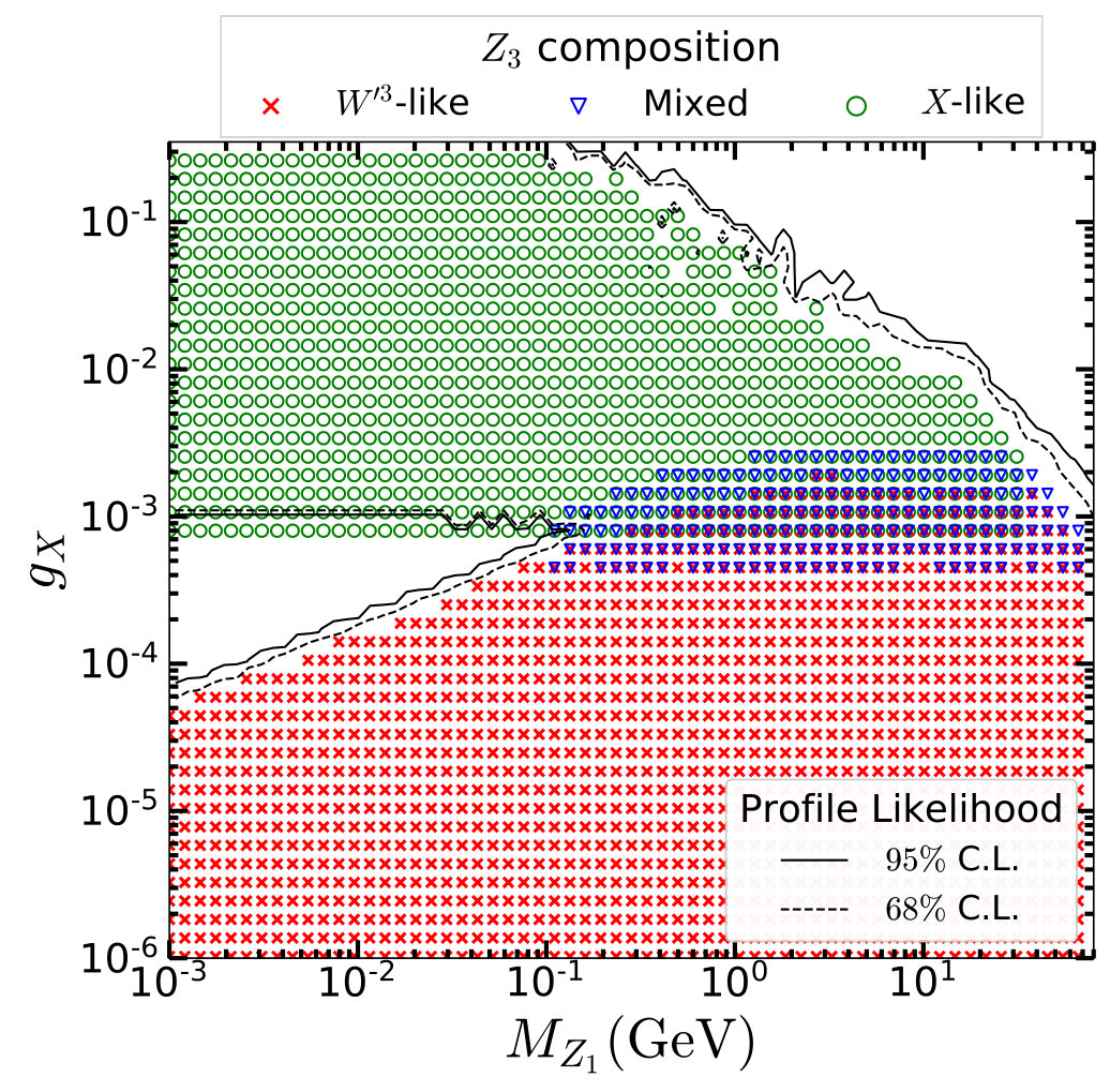 Figure 16
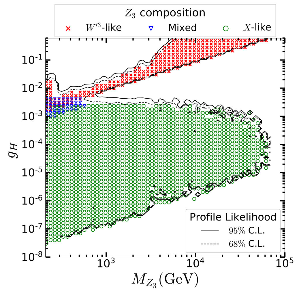 Figure 17
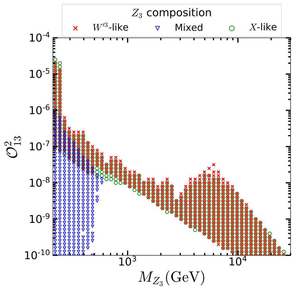 Figure 18
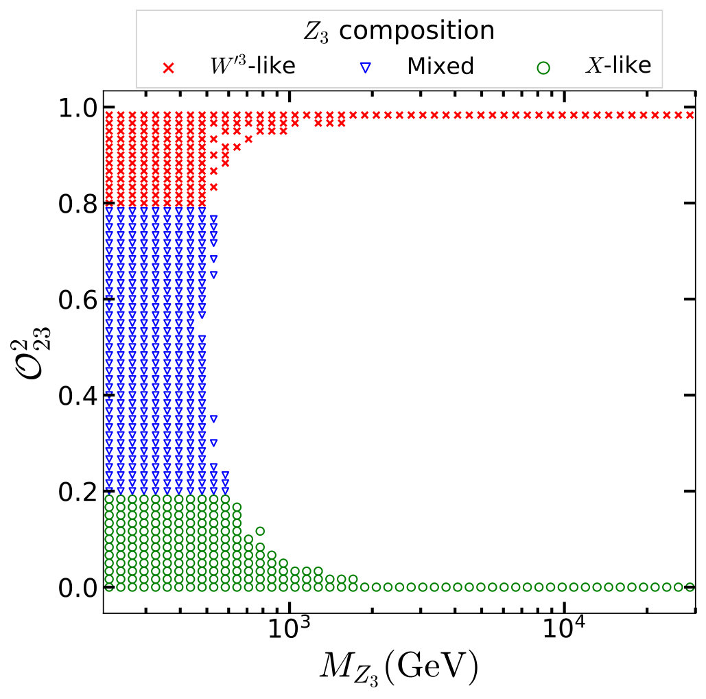 Figure 19
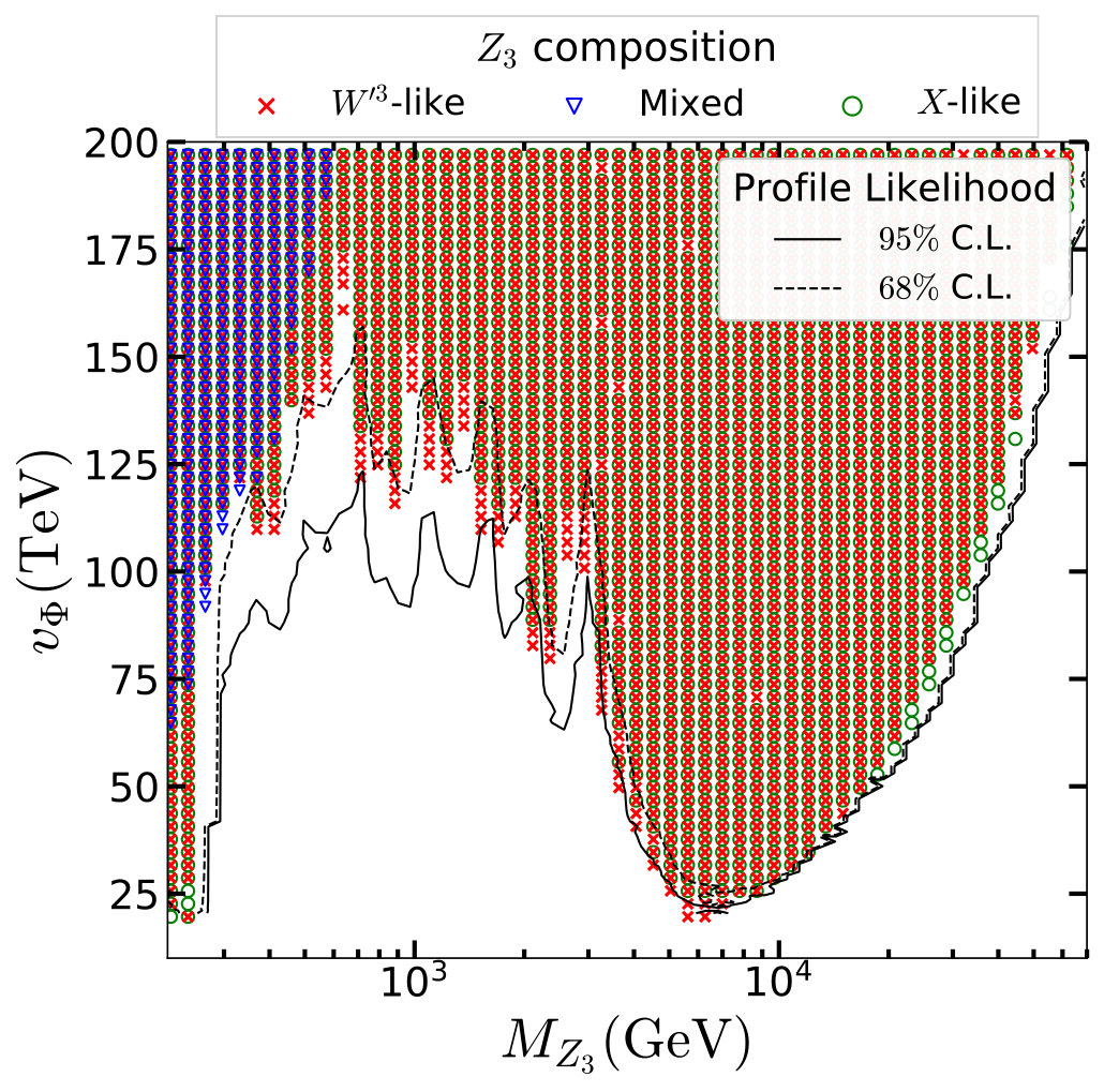 Figure 20
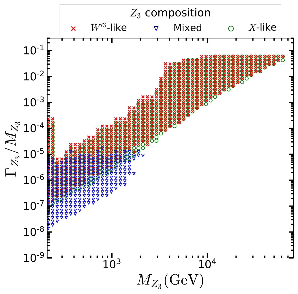 Figure 21
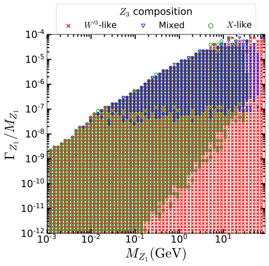 Figure 22
| Fields | Spin | |||||
|---|---|---|---|---|---|---|
| 0 | 1 | 2 | 2 | |||
| 0 | 1 | 1 | 3 | 0 | 0 | |
| 0 | 1 | 1 | 2 | 0 | ||
| 3 | 2 | 1 | 0 | |||
| 3 | 1 | 2 | ||||
| 3 | 1 | 2 | ||||
| 3 | 1 | 1 | 0 | |||
| 3 | 1 | 1 | 0 | |||
| 1 | 2 | 1 | 0 | |||
| 1 | 1 | 2 | 0 | |||
| 1 | 1 | 2 | ||||
| 1 | 1 | 1 | 0 | 0 | ||
| 1 | 1 | 1 | 0 | |||
| 1 | 8 | 1 | 1 | 0 | 0 | |
| 1 | 1 | 3 | 1 | 0 | 0 | |
| 1 | 1 | 1 | 3 | 0 | 0 | |
| 1 | 1 | 1 | 1 | 0 | 0 | |
| 1 | 1 | 1 | 1 | 0 | 0 |
| Observables | LEP Data | CEPC Precision CEPC-SPPCStudyGroup:2015csa | Standard Model |
|---|---|---|---|
| [GeV] | 91.1876 0.0021 | 91.1884 0.0020 | |
| [GeV] | 2.4952 0.0023 | 2.4942 0.0008 | |
| [GeV] | 1.7444 0.0020 | — | 1.7411 0.0008 |
| [MeV] | 499.0 1.5 | — | 501.44 0.04 |
| [MeV] | 83.984 0.086 | — | 83.959 0.008 |
| 41.541 0.037 | — | 41.481 0.008 | |
| 20.804 0.050 | — | 20.737 0.010 | |
| 20.785 0.033 | 20.737 0.010 | ||
| 20.764 0.045 | 20.782 0.010 | ||
| 0.21629 0.00066 | 0.21582 0.00002 | ||
| 0.1721 0.0030 | — | 0.17221 0.00003 | |
| 0.0145 0.0025 | — | 0.01618 0.00006 | |
| 0.0169 0.0013 | — | 0.01618 0.00006 | |
| 0.0188 0.0017 | — | 0.01618 0.00006 | |
| 0.0992 0.0016 | 0.1030 0.0002 | ||
| 0.0707 0.0035 | — | 0.0735 0.0001 | |
| 0.0976 0.0114 | — | 0.1031 0.0002 | |
| 0.15138 0.00216 | — | 0.1469 0.0003 | |
| 0.142 0.015 | — | 0.1469 0.0003 | |
| 0.136 0.015 | — | 0.1469 0.0003 | |
| 0.923 0.020 | — | 0.9347 | |
| 0.670 0.027 | — | 0.6677 0.0001 | |
| 0.0895 0.091 | — | 0.9356 |
Peer Reviews
No public reviews on file for this paper yet. If you reviewed it on a platform where reviews are public (OpenReview, ICLR, NeurIPS, ICML), you can paste yours below so the community can read it here.
Videos
No videos yet. Explain this paper in a talk, walkthrough, or lecture? Add one.
Consistency of Gauged Two Higgs Doublet Model:
Gauge Sector
Cheng-Tse Huang1, Raymundo Ramos2,
Van Que Tran2,3, Yue-Lin Sming Tsai2,4 and Tzu-Chiang Yuan2
1Interdisciplinary Program of Sciences, National Tsing Hua University, Hsinchu 30013, Taiwan
2Institute of Physics, Academia Sinica, Nangang, Taipei 11529, Taiwan
3School of Physics, Nanjing University, Nanjing 210093, China
4Key Laboratory of Dark Matter and Space Astronomy, Purple Mountain Observatory, Chinese Academy of Sciences, Nanjing 210008, China
Abstract
We study the constraints on the new parameters in the gauge sector of gauged two Higgs doublet model using the electroweak precision test data collected from the Large Electron Positron Collider (LEP) at and off the -pole as well as the current Drell-Yan and high-mass dilepton resonance data from the Large Hadron Collider (LHC). Impacts on the new parameters by the projected sensitivities of various electroweak observables at the Circular Electron Positron Collider (CEPC) proposed to be built in China are also discussed. We also clarify why the Stüeckelberg mass for the hypercharge is set to be zero in the model by showing that it would otherwise lead to the violation of the standard charge assignments for the elementary quarks and leptons when they couple to the massless photon.
I Introduction
The discovery of the 125 GeV scalar boson identified as the Higgs boson in the Standard Model (SM) Salam:1959zz ; Glashow:1961tr ; Weinberg:1967tq ; Salam suggested that the simple Higgs mechanism Englert:1964et ; Higgs:1964pj ; Guralnik:1964eu for electroweak symmetry breaking proposed by Weinberg Weinberg:1967tq and Salam Salam is the choice by nature. Both Run I and Run II data collected by the two experimental groups ATLAS and CMS at the Large Hadron Collider (LHC) reveal no significant deviations from the SM predictions. Alternative models for electroweak symmetry breaking like technicolor or composite Higgs models are arguably more elegant but necessarily more complicated. Simplicity seems to be more superior over other criterion like complexity or elegance for model buildings.
Nevertheless experimental observations of neutrino oscillations imply there must be new physics beyond the SM to account for the minuscule masses of neutrinos. Missing mass problem and cosmic acceleration of our universe also suggested the introduction of dark matter (DM) Lin:2019uvt and dark energy Peebles:2002gy . The standard CDM model of cosmology Dodelson:2003ft consists of the SM of particle physics plus two new ingredients, namely the cold dark matter, which can be the weakly interacting massive particle predicted by many new particle physics models, and a tiny positive cosmological constant at the present time in the Einstein’s field equation for gravity, which can be mimicked by numerous models of dark energy. Many models of dark matter and neutrino masses require extension not only of the simple Higgs sector but sometimes also the electroweak gauge sector of the SM as well. Moreover, models of dark energy are often represented by new scalar field with equation of state that can provide negative pressure in order to explain the cosmic acceleration at late times.
Thus extension of the SM in one way or the other seems necessary if one wants to solve the above puzzles in the neutrino sector and in cosmology. At the same time, one should be open-minded that there might be other approaches other than particle physics to answer some of these questions and remembering that nature is the ultimate arbiter of all theoretical imaginations.
The gauged two Higgs doublet model (G2HDM) proposed in Huang:2015wts was motivated partly by the inert Higgs doublet model (IHDM) Deshpande:1977rw ; Ma:2006km ; Barbieri:2006dq ; LopezHonorez:2006gr of dark matter. IHDM is a variant of the general 2HDM Branco:2011iw with an imposed discrete symmetry on the scalar potential and the Yukawa couplings such that one of the Higgs doublets is odd and become a scalar dark matter candidate. Dangerous tree level flavor changing neutral current (FCNC) interactions in the Yukawa couplings, generally presence in the general 2HDM, are also eliminated by this discrete symmetry. Due to its relatively simple extension of the SM, many detailed analysis of IHDM had been done in the literature Arhrib:2013ela ; Arhrib:2014pva ; Ilnicka:2015jba ; Belyaev:2016lok ; Eiteneuer:2017hoh ; Borah:2018rca ; Kephart:2015oaa ; Goudelis:2013uca ; Swiezewska:2012eh ; Arhrib:2012ia . In G2HDM, the discrete symmetry in IHDM was not enforced. Instead the two Higgs doublets and are grouped into a two-dimensional irreducible representation of a new gauge group . A priori there is no need to impose the discrete symmetry in G2HDM. Once we write down all renormalizable interactions for G2HDM, this discrete symmetry emerges as an accidental symmetry automatically. Tree level flavor changing neutral current (FCNC) interaction in the Higgs-Yukawa couplings are also absence naturally for the SM fermions. As long as one does not break this symmetry spontaneously, which might lead to the domain wall problem in early universe, the doublet is naturally an inert Higgs doublet and can play some role in dark matter physics. It is more satisfactory to have a global discrete symmetry like the parity that guarantees the stability of dark matter embedded into a local symmetry. Indeed there exists theoretical arguments showing that global continuous or discrete symmetries are not compatible with quantum gravity Krauss:1988zc ; Kallosh:1995hi . Detailed analysis of the complex scalar dark matter physics in G2HDM will be presented in a forthcoming paper DMPaper .
The construction of G2HDM in Huang:2015wts involves extension of both the Higgs and gauge sector of the SM which we will discuss shortly in the next section. Several phenomenological implications of G2HDM had been explored in Huang:2015rkj ; Huang:2017bto ; Arhrib:2018sbz ; Chen:2018wjl . In particular, we have studied recently in details the theoretical and phenomenological constraints on the scalar sector Arhrib:2018sbz .
We note that the 2HDM augmented with an extra local abelian has been discussed in the literature Ko:2012hd ; Campos:2017dgc ; Camargo:2018klg ; Camargo:2018uzw ; Camargo:2019ukv ; Cogollo:2019mbd to address neutrino masses, dark matter and to avoid FCNC interactions at the tree level.
As mentioned before, all experimental data are in line with SM predictions. The extended gauge sector of G2HDM must be challenged by electroweak precision test (EWPT) data obtained previously at LEP-I and LEP-II as well as current data at the LHC. Constraints must be imposed on the new parameters in the extended gauge sector of G2HDM. The main purpose of this work is to study these constraints on the gauge sector systematically in analogous to previous analysis Arhrib:2018sbz done for the scalar sector. It is also interesting to address the sensitivities of these new parameters at the future colliders.
The contents of this paper is organized as follows: In the next Sec. II, we review the G2HDM and highlight some of its crucial features of the gauge sector relevant most to this work. Sec. III discusses the experimental constraints, including the electroweak precision test constraints at and off the -pole at LEP, Drell-Yan data from on-shell decay of the boson at the LHC, and the full LHC Run II data from the high-mass dilepton resonance of an extra neutral gauge boson . Sec. IV contains our numerical results from the profile likelihood analysis. We also study future sensitivities of the new parameters in future experiments, in particular for the Circular Electron Positron Collider (CEPC) CEPC-SPPCStudyGroup:2015csa proposed/debated to be built in China. Finally, we summarize and conclude in Sec. V. In Appendix A we present the formulas for the mixing angles among the three massive neutral gauge bosons in G2HDM in terms of the fundamental parameters in the Lagrangian of the model. The dominant two-body decay widths for the two new neutral gauge bosons are discussed in Appendix B.
II G2HDM Set Up
In this section, we will start with a brief review for the set-up of G2HDM Huang:2015wts by specifying its particle content (Sec. II.1) and then write down the mass spectrum of the neutral gauge bosons (Sec. II.2) and their interactions with the SM fermions (Sec. II.3) in the model. Along the way, we will discuss some peculiar effects for nonzero Stüeckelberg mass associated with the hypercharge .
II.1 Particle Content
The particle content of G2HDM is listed in Table 1 111 in the table were denoted as respectively in Huang:2015wts .. Besides the two Higgs doublets and combining to form in the fundamental representation of an extra , we introduced a triplet and a doublet of this new gauge group. However and are singlets under the electroweak SM gauge group . Only carries both quantum numbers of the and .
There are different ways of introducing new heavy fermions in the model but we choose a simple realization: the heavy fermions together with the SM right-handed fermions comprise doublets, while the SM left-handed doublets are singlets under . We note that heavy right-handed neutrinos paired up with a mirror charged leptons forming doublets was suggested before in the mirror fermion model Hung:2006ap . To render the model anomaly-free, four additional chiral (left-handed) fermions for each generation, all singlets under both and , are included. For the Yukawa interactions that couple among the fermions and scalars in G2HDM, we refer our readers to Huang:2015wts for more details, since they are not relevant to this work.
To avoid some unwanted pieces in the scalar potential and Yukawa couplings, we require the matter fields to carry extra local charges. Thus the complete gauge groups in G2HDM consist of . Apart from the matter content of G2HDM, there also exist the gauge bosons corresponding to the SM and the extra gauge groups.
The salient features of G2HDM are: (i) it is free of gauge and gravitational anomalies; (ii) renormalizable; (iii) without resorting to an ad-hoc symmetry, an inert Higgs doublet can be naturally realized, providing a DM candidate; (iv) due to the nonabelian gauge symmetry, dangerous FCNC interactions are absent at tree level for the SM sector; (v) the VEV of the triplet can trigger symmetry breaking while that of provides a mass to the new fermions through -invariant Yukawa couplings; etc.
II.2 Neutral Gauge Boson Masses
Consider the interaction basis for the neutral gauge bosons and denote their mass eigenstates as . After spontaneous symmetry breaking, the 44 mass matrix in the interaction basis of is given by Huang:2015wts
[TABLE]
Here , , and denote the gauge couplings of , , and respectively; and are the vacuum expectation values (VEVs) of and respectively; and are the Stüeckelberg masses for the two abelian and respectively. We note that the VEV of the triplet does not enter into the neutral gauge boson mass matrix. This is unlike the case of scalar boson mass matrix analyzed in Arhrib:2018sbz which involves all three VEVs, , and . The matrix in Eq. (1) is real and symmetric and thus can be diagonalized by a 44 orthogonal rotation matrix that we will denote as
[TABLE]
where . The zero mass state is naturally identified as the photon.
Some comments on the Stüeckelberg masses and are in order here. It has been demonstrated in Ruegg:2003ps that for the extension of SM with a Stüeckelberg mass for the hypercharge , there exists a plethora of new physical effects. Notably, besides the photon obtaining a mass, neutrinos will couple to the photon and charged leptons will have axial vector couplings with the photon. Nevertheless, the Stüeckelberg extension of the SM doesn’t spoilt renormalizability of the model. All these new effects are proportional to . Experimentally, the photon mass upper bound deduced from modeling the solar wind in magnetohydrodynamics is eV Tanabashi:2018oca , which implies must be very tiny too. If individual Stüeckelberg mechanism is introduced for each of the two s factors in G2HDM, the photon will in general obtain nonzero mass and many results obtained in Ruegg:2003ps apply as well. In Huang:2015wts , we followed Kors:2005uz ; Kors:2004iz ; Kors:2004ri ; Kors:2004dx in which only one Stüeckelberg field was introduced for the two factors of s to implement the Stüeckelberg mechanism. The matrix thus obtained given in Eq. (1) has zero determinant and a massless photon can always be realized for arbitrary values of the Stüeckelberg masses and .
In the next subsection, we will show that with a nonzero the electric charge assignments of the SM fermions and their heavy partners in G2HDM will no longer be standard but instead receive milli-charge corrections like those discussed in Ruegg:2003ps . In particular, neutrinos will couple to the photon and all fermions also have axial vector couplings with the photon at tree level. These peculiar effects depend on through the mixing matrix elements and hence necessarily small. Thus, we have strong theoretical motivation to set in what follows to avoid these unpleasant features. For an analysis with both and nonzero in a Stüeckelberg extension of the SM that maintains the standard QED interaction for the SM fermions, see Feldman:2007nf ; Feldman:2007wj ; Feldman:2006wb . The main reason why the photon-fermion couplings in G2HDM are in general different from these previous works is due to the presence of the extra gauge group whereas there is only one extra abelian group in Feldman:2007nf ; Feldman:2007wj ; Feldman:2006wb .
Setting in G2HDM will simplify and allows us to write the rotation matrix in the following product form
[TABLE]
where and represent and respectively, with being the Weinberg angle defined by
[TABLE]
It is obvious that the matrix in Eq. (3) is just the product of the SM gauge rotation matrix made into a matrix, called , times a general orthogonal rotation matrix which was also converted to a matrix. After applying the rotation to , the result is
[TABLE]
where is the mass of the boson in the SM. We can consider the vanishing (1,1) element to be the mass of the photon eigenstate . Furthermore, according to Eqs. (2) and (3), the remaining 33 matrix formed by the non-vanishing elements above is diagonalized by the orthogonal matrix . In particular, one can parametrize in terms of the following Tait-Bryan representation
[TABLE]
where and stand for sine and cosine with the rotation angle respectively. As shown in Appendix A, these rotation angles can be represented as
[TABLE]
[TABLE]
[TABLE]
It is easy to see that taking the limits of and go to 0, the non-vanishing 33 block matrix in Eq. (5) becomes . Thus the rotation matrix must be identity. This can be realized by setting , and to be zeros which can be derived from Eqs. (7), (8) and (9).
We note that if one sets to zero, the mass matrix in the right-handed side of Eq. (5) is symmetric under the interchange of .
After the rotation matrix is found, the mass eigenstates where runs from 1 to 3 are given by
[TABLE]
The composition , and of the mass eigenstate is given by , , and , respectively. In general, the -pole can be any one of the depending on which one is actually closer to the pole by the underlying parameter choices in G2HDM. In our analysis, we will consider there is always at least one extra neutral gauge boson heavier than the -pole.
II.3 Neutral Gauge Current Interactions
The part of the Lagrangian that contains the interaction of the with visible matter in G2HDM is
[TABLE]
where . The and factors are given by ()
[TABLE]
Here is the isospin charge and is the electric charge in units of for the SM fermion where is given by Eq. (4). They are related to the hypercharge by the standard formula . The charges due to the new gauge symmetries are as the charge of the corresponding and is the analogous of the isospin again for the corresponding . We simply define depending on belongs to the upper or lower component of an doublet.
For the photon-fermion couplings in G2HDM, we obtain
[TABLE]
where
[TABLE]
Thus, with both nonzero and , the electromagnetism interaction in G2HDM is in general different from the SM case. The standard charge assignment for every SM fermion will suffer from an overall correction factor of plus two correction terms, and there is also a non-vanishing axial vector coupling.
Next, we can take the limit and write the corresponding expressions. By replacing the elements of by and as in Eq. (3), one can find the following new expressions for the vector and axial vector couplings
[TABLE]
Similarly, one can do the same substitutions on Eqs. (II.3) and (II.3) together with and check that the photon coupling to the SM fermions goes back to the SM expression while all the axial vector couplings vanish. This is the main physical reason why we set so as to reproduce the standard photon-fermion couplings. For , it can be arbitrary and is naturally to consider the light and heavy scenarios where it is smaller and greater than the -boson mass respectively.
Obviously, the formulas obtained in this subsection for the couplings of the neutral gauge bosons with the SM fermions also hold for the heavy fermions in G2HDM.
III The Constraints
III.1 Constraints from Precision Electroweak Data at LEP-I
The interaction of boson with SM fermions is described by the Lagrangian in Eq. (11). For the case of limit, the tree-level couplings are shown in Eqs. (17) and (18). For more precise calculation, we include the radiation corrections from propagator self-energies and flavor specific vertex corrections to the boson and fermions couplings Erler:2004nh ; ALEPH:2005ab , which now are given by 222We ignore loop corrections related to the new gauge couplings and . (suppressing in the subscripts)
[TABLE]
where in this work is either equal to 1 or 2 depending which mass eigenstate is closest to -pole. The parameters and are loop corrections quantities. The decay of the boson into fermions and anti-fermions in the on-shell renormalization scheme is given by Baur:2001ze ; Erler:2004nh
[TABLE]
where is the color factor (1 for leptons and 3 for quarks), , and
[TABLE]
with
[TABLE]
Here is the electric charge of the fermion in unit of , and and are the fine-structure and strong coupling constants, respectively, evaluated at the scale. It is understood that the couplings and in Eq. (21) should be replaced by and in Eqs. (19) and (20) respectively with or 2 depending which is closest to the -pole .
We also investigate some -pole () observables, including the ratio of partial decay width of boson
[TABLE]
the hadronic cross-section
[TABLE]
the parity violation quantity
[TABLE]
and the forward-backward asymmetry quantity
[TABLE]
where is the initial polarization. Recall that at LEP-I , in this case
[TABLE]
A summary of the electroweak observables at -pole from various experiments Tanabashi:2018oca is presented in Table 2.
From the data in Table 2, we build the Chi-squared for the electroweak observables at -pole as follows
[TABLE]
Note that we have considered the correlations between the total decay width of boson and its partial decay widths to hadrons, invisibles and dilepton. For each on the right-handed side of Eq. (30), it is given by the standard expression, namely
[TABLE]
where represents the experimental/theoretical value of any one of the 23 electroweak observables listed in Table 2 and is the corresponding experimental uncertainty.
III.2 Contact Interactions at LEP-II
We also include constraints from data above the -pole by considering the LEP-II measurements related to contact interactions taking the following form of effective Lagrangian
[TABLE]
where represent the chirality projection operators with being or for left-handed or right-handed fermions, respectively. The sign of Eq. (32) depends on whether the interference between the contact interaction it parametrizes and the SM process is constructive () or destructive (). There is a total of 6 combinations for the indices of : , which are also called models. The limits on set by LEP-II are given in Table 3.15 of Ref. Schael:2013ita . The strongest constraint is given by TeV. By using these values, we are able to reconstruct the cross section for new physics processes based on the Lagrangian in Eq. (32).
To improve the analysis of this section, in particular for the cases where the mass of one of the gauge bosons is below the -pole, we calculate the additional -like mediator contribution 333 In what follows, we will denote the extra neutral gauge boson as or depending on whether we refer to the experimental data or G2HDM. to the scattering cross section. In the case we have the contribution of both and channels while for only the channel contributes. Note that here we do not need the SM contributions such as the photon and exchange not considered in Eq. (32). In the massless approximation for all the external fermions, the amplitudes for the and channels and for the interference term between them are given by:
[TABLE]
where is the center of mass energy squared, and is the angle between incoming and outgoing particles. This angle should be integrated to obtain the final cross section. The resulting cross section has to be compared against the cross section obtained using the effective Lagrangian in Eq. (32) with the given by the experimental result. The couplings and have 1 or 2 depending on whether we are analyzing light or heavy scenario. For , we assume is much heavier than so that its contributions are negligible. To be able to construct a from the LEP-II 95% C.L. limit, we calculate the corresponding 95% C.L. cross section and compare against the theoretical result. When our theoretical result matches the 95% C.L. with null-signal assumption, the corresponding value should be 2.71 444 For a Gaussian distribution, the value of corresponds to the 90% C.L. of a two-tailed test, but it also equivalent to the 95% C.L. of a one-tailed test that we are using. . In this case, we calculate the value using
[TABLE]
where is the cross section obtained using the effective Lagrangian of Eq. (32) with the experimental results for given in Ref. Schael:2013ita for different combinations of the chirality. The effective cross sections for different combinations of from the data are summed and averaged. We do not consider the combinations of VV and AA since they are not independent from the other polarizations considered above. Note that Eq. (36) goes to zero when the theoretical cross section vanishes (SM limit) as one would expect.
In the light scenario (see Sec. IV.3) in which one of the new neutral gauge boson is too light and invalidates the effective contact interaction approach, it is mandatory to recast the LEP-II constraints for the contact interactions into the cross section level to do the analysis. We checked that for the heavy scenario, using either the effective contact interaction or cross section approach give the same results.
III.3 Drell-Yan Constraints at the LHC
In this section we recap the experiments of the Drell-Yan cross section for SM -boson and heavy at the LHC.
III.3.1 -boson on-shell decay at the LHC
By using the measurement of the Drell-Yan cross section for the -boson production, the properties of the are well determined at the LHC. Among all the final states of the -boson decay, the dilepton signature is the most relevant to distinguish signal from background. It is commonly believed that the Drell-Yan constraint from the LHC is weaker than LEP EWPT data because of the relative larger uncertainties from the hadronic background than the QED background. However, to be careful, we first check a direct Drell-Yan constraints from the LHC Aaboud:2017buh . The data of electron-positron pair () and muon-pair () final states are given by Tables 3 and 4 respectively in Ref. Aaboud:2017buh . In the signal region located around -boson mass (the invariant mass ), we found that the systematic uncertainties of Drell-Yan background is larger than the data statistic uncertainties in both or final state. We have also checked that the EWPT constraints in Table 2 are much stronger than LHC Drell-Yan constraint.
On the other hand, -boson can be singly produced either by radiation from the incoming partons (Fig. 1a) or -channel exchange of a gauge boson (Fig. 1b). To constrain the G2HDM modified couplings, the later process is more useful than the former because QCD processes usually suffer from larger systematical uncertainties than the electroweak ones. Recently, ATLAS Aaboud:2017emo reported a fiducial electroweak cross section of fb and fb for dijet invariant masses greater than and , respectively. The SM simulated cross sections are also given in Table 5 of Ref. Aaboud:2017emo , where central values and the uncertainties are given as fb for and fb for .
Comparing with the SM, except for the couplings, the G2HDM did not modify much of the cross section. Namely, the electroweak cross section of the G2HDM version can be simply rescaled as
[TABLE]
where
[TABLE]
and . However, similar to direct Drell-Yan boson search, we found that the value of is not easy to derivate from unity and the power of constraining the parameter space in G2HDM is not as strong as LEP EWPT constraints.
Finally, we have numerically verified that the allowed G2HDM parameter space is hardly changed at all whether the direct and electroweak Drell-Yan boson constraints at the LHC are included or not. Again, this is because both constraints at the LHC are much weaker than LEP EWPT constraints. Hence, we will not take into account the LHC Drell-Yan constraints from the on-shell decay in our numerical works so as to save some computer resources.
III.3.2 LHC Boson Search at High-mass Dilepton Resonances
The Drell-Yan constraints can also be very powerful for the new gauge bosons in G2HDM once they can be singly produced Huang:2017bto . Unlike the study in Ref. Huang:2017bto which only -like is considered, we extend it here to any with all the possible composition. Recently, ATLAS collaboration Aad:2019fac reported a new result on dilepton resonances with the integrated luminosity of fb*-1* and the center-of-mass energy . They indicated that the lower limit on the mass of boson for a simplified model can be raised up to . Considering this new measurement, we update the constraints of the heavy neutral gauge boson masses in G2HDM and the upper limits of and .
In Fig. 3 of Ref. Aad:2019fac , one can see the upper limits of cross section times branching ratio BR() are based on the ratio of the total width of divided by its . Depending on this ratio, the limits can be altered by a factor of . As shown in Appendix B, the in the G2HDM shall be always less than . Hence, for a conservative approach, we can simply apply the ATLAS result by using their upper limit associated with .
Furthermore, the total decay width relies on whether decays to the new particles in G2HDM. The heavy new fermions in G2HDM are assumed to be very heavy so that they do not affect the EW-scale physics in any significant way. On the other hand, the invisible decay to a scalar DM pair can be a more important channel because the upper limits of various parameters can be weaker than the one without taking into account the decays to the DM pair. The openings of the scalar channels as well as other channels with one vector and one scalar particles in the final states of decay makes the parameter spaces of the gauge and scalar sectors entangle with each other. Thus a complete analysis becomes quite formidable. In Eq. (76), one can see that the invisible decay width of has two different limits, for maximum invisible decay and for zero invisible decay. For the sake of simplicity, we will be contented by presenting the results based on these two benchmark invisible decay widths. In this study, we adopt for maximum invisible decay but we found that the can differ within an accepted range of comparing with the massless case.
Using MadGraph5 Alwall:2014hca , we compute the cross section . Since we enforce that the cross section is computed at the resonance, we only used a minimum cut given by the default parameter card in MadGraph5. It is very CPU time consuming to estimate the cross section point by point throughout all the parameter space. Nevertheless, the cross section can be obtained by simply rescaling the vector and axial vector couplings and using Eqs. (17) and (18). Hence, by using the same reasoning as before we include the latest ATLAS limit in our scan by using the following chi-squared function
[TABLE]
where the branching ratio can be found in Appendix B and is C.L. taken from the curve associated with in Fig. 3 of Ref. Aad:2019fac .
IV Results
IV.1 Numerical Methodology
Our aim is to determine the and allowed parameter space of the G2HDM which are favored by all of the experimental data presented in the previous section. In this paper, we will use the profile-likelihood (PL) method to perform the statistical data analysis. We recap the PL method in the following. Briefly, the PL method is a well popular statistical method to deal with the multi-dimensional parameter space which treats the unwanted parameters as nuisance parameters. In other words, if a proposed model has -dimensional parameter space and we are only interested in of those dimensions, then the PL method can remove the unwanted dimensions which we are not interested in, by maximizing the likelihood over them.
There are 4 new parameters in the gauge sector of G2HDM. They are the two new gauge couplings and and the two new scales and . Our results will be presented in two-dimensional parameter regions with 68% and 95% confidence levels (C.L.). Take the plane () as an example. After marginalizing over the other two parameters and , an integral of the likelihood function can be written as
[TABLE]
where is the smallest area bound with a fraction of the total probability and the normalization in the denominator is the total probability with .
The total we will use in our analysis is the sum of Eqs. (30), (36), and (39), namely
[TABLE]
where we have suppressed the arguments of all the functions. We adopt the statistical sensitivity as
[TABLE]
Since our likelihood is modeled as a pure Gaussian distribution, i.e. , one can connect the to the confidence level: the 68% (95%) C.L. in a two dimensional parameter space corresponding to . Here is the maximum value of the likelihood in the region .
There are two interesting scenarios: (i) heavy and (ii) light . The heavy scenario will result in two new heavy neutral gauge bosons and , and the measured boson located at -pole will be the lightest one, . However, the light scenario will result in a new boson lighter than the -pole which is usually called dark () or dark photon (). In this case, corresponds to the -pole and . Hence, we choose our scan ranges for two scenarios,
[TABLE]
For the other three parameters, we use the same ranges for the two scenarios of 555 There is also the possibility of both and are light, which may lead to and both and are lighter than . We will reserve this interesting scenario in future work.,
[TABLE]
We perform random scans by using MultiNest v2.17 Feroz:2008xx with 30000 living points, an enlargement factor reduction parameter 0.5 and a stop tolerance factor . For sampling coverage, we combined several scans and finally obtained samples for each scenario.
IV.2 Heavy Scenario
In the heavy scenario, the mass of boson is located at around -pole () so that is identified as the SM -boson. Note that boson physics is strongly affected by the different composition of () but not the heaviest boson () because is heavier than in our parameter choices and therefore has less impact.
In Fig. 2, we present the scatter points of the composition of for the region based on the likelihoods described in Sec. IV.1. The color code hereafter represents the three different composition of . Recalling Eq. (10), we define -like with condition (red crosses ), mixed state with (blue triangles ), and -like with condition (green circles ).
The allowed scatter points projected on the (, ) and (, ) planes are depicted in Figs. 2a and 2b, respectively. From the density of distribution in Fig. 2a, we can clearly see that the mixed state (blue triangles) is less evenly distributed because it needs some trade-off between the two new gauge couplings and . In Fig. 2b, we projected the same parameter space on the plane (, ). Note that the mixing presents how is consisted of . Therefore, very small implies from the orthogonality of . Furthermore, the upper limit of sets an lower limit of the for the red cross region. If goes to infinity, becomes super heavy and decouple. The composition of in should then be negligible, thus vanishes in this limit. We note that the excluded concave up region of between 250 GeV and 6 TeV on the upper limit of is due to the constraint from ATLAS search.
In Fig. 3, we show the (dashed) and (solid) likelihood contours with scatter points inside the region on the (a) (, ) and (b) (, ) planes. In Fig. 3a, we can see that the -like red crosses form a band with a tendency proportional to . This is because for a -like , which can be extracted from the (3,3) element of the mass matrix in Eq. (5). We can also see that at the lower bound of this band, the 95% and 68% C.L. contours are overlapped because this lower bound is due to our choice of in its upper scan range, not from the likelihood results. This implies that in the upper edge of this red band where has larger value, the value of there is smaller. Therefore, the upper bound of this red cross band corresponds to the lower values of , which can be excluded by the tolerance as we can see in Fig. 3b where the scatter plot is projected on the (, ) plane. Surprisingly, in Fig. 3a, the blue triangle band, corresponding to mixing mostly between and bosons, matches the red cross band. This can be understood as the mass of being dominated by the (3,3) element of Eq. (5) even for an boson composition. In the same figure, we can see the green circles running from below the two red cross and blue triangle bands up to the upper limit of . In other words, we can see how the passes from being dominated by the (3,3) element of Eq. (5) (red crosses), which is -dependent, to being dominated by the -independent (4,4) element (green circles).
One particular feature of Fig. 3b is that the low and low region (lower left corner) is covered only with -like points while both -like and mixed points only approach this corner down to a curved bound. This curved section in the lower bound can be related to the curved upper bound for and mixed points in Fig. 3a for low GeV and . These curves in the upper bound (Fig. 3a) and in the lower bound (Fig. 3b) can be understood as smaller requiring larger to pass EWPT. In particular, if is small, has to be large in order to have a sizable diagonal (3,3) element in the mass matrix in Eq. (5), while the off-diagonal (2,3) and (3,2) elements remain small. However, the mixing effects from the off-diagonal elements are not negligible and expected to be stronger when the mass is getting closer to the mass. This gives rise to the upper and lower bounds that we see in Figs. 3a and 3b, respectively, for the -like points. Such behaviour is not displayed for the -like points since they do not depend strongly on .
The ATLAS constraint almost rules out the region for -like and mixed , except the region with . However, the -like at the same region has not been affected much by the ATLAS constraint.
Similarly, in Fig. 4, we show the (dashed) and (solid) likelihood contours with scatter points inside the region on the (a) (, ) and (b) (, ) planes. From Fig. 4a, one can easily see that the -like boson (green circles) forms a band whose tendency is proportional to the . This can be understood by the fact that the composition of the in this case is mainly from , which has a mass proportional to again coming from the (3,3) element of the mass matrix in Eq. (5). On the other hand, in the case of the -like boson (red crosses), the mass of the almost does not depend on . Indeed, the composition of is now mainly from and . This is clearly shown in Fig. 4b, when is small (), the mass of in the red cross region is dominated by and less than our set-up limit of GeV. However, when is getting bigger, the mass of the can be dominated by the term for sufficiently large value of . We can also see that the EWPT data sets upper bounds on and . The excluded concave up region of in Fig. 4a for the -like and mixed composition of is again due to the ATLAS search which does not apply for the -like case. As a result, the ATLAS search cannot constrain on for -like points as clearly shown in Fig. 4b.
IV.3 Light Scenario
In the light scenario, we require that the mass of boson is always at around -pole (). In this scenario, the lightest with mass less than the -boson mass can be the dark photon or dark , while the conventional is the heaviest boson . We note that the composition of is given by . The allowed scatter points projected on the (, ) and (, ) planes are depicted in Figs. 5a and 5b, respectively. The color code for the composition of is the same as in Fig. 2 for .
An obvious feature of Fig. 5a is that the mixed state of (blue triangles) has a mass upper limit. Intuitively, it requires some trade-off between the gauge couplings and which results in . This effect will be discussed with more detail later in Fig. 6. In Fig. 5b, we can see that the composition of is again small. However, unlike the heavy scenario, the -like boson has a similar distribution as -like boson. Additionally, the mixed state at the mass region between and cannot be excluded by the ATLAS constraint which is also different from the heavy scenario.
In analogous to Fig. 3, we show in Fig. 6 the (dashed) and (solid) likelihood contours with scatter points in the region on the (a) (, ) and (b) (, ) planes. Comparing Figs. 3a and 6a, we have a clear separation between the -like (red crosses) and -like (green circles) regions in this light scenario. As before, the -like red crosses follow a tendency proportional to again because of the dominance of the (3,3) element of Eq. (5) in , i.e., . Other features shared between -like points in Figs. 3a and 6a are the distribution of values; the lower bound owes to upper bound but its upper bound owes to tolerance. As expected, the ATLAS search can constrain and at the mass region . However, the gauge coupling for -like is proportional to not so that the ATLAS search cannot constrain on at the -like region, indicated by green circles. The -like region in Fig. 6a has a upper bound around given by the tolerance and most likely related to the lower bound on displayed on Fig. 6b. The mass of , , in this -like green region can be approximated by , this is why there is not a clear dependence as in the -like points. In Fig. 6a, as one would expect, the mixed region corresponds approximately to the intersection between -like and -like regions, extending lightly into their exclusive regions. This means that the upper and lower bound of the mixed region are approximately given by the upper bound of the -like region and the lower bound of the -region, respectively. If we increase our maximum value, the lower bound of the -like region would reach lower and the maximum for the mixed region would be increased. This is more clear after looking at Fig. 6b where the maximum value for the three regions grows with the value of .
Similarly, in Fig. 7, we show the (dashed) and (solid) likelihood contours with scatter points in the region on the (a) (, ) plane and (b) (, ) planes. Again, the red cross represents the points of -like boson, the blue triangle represents the points of mixed state (, and ) boson, and the green circle represents -like boson. We note that in this scenario, is considered as a dark photon 666The lightest boson can be tested in the dark photon experiments but it is beyond the scope of this work. We will return to this in the future. and has mass range from 1 MeV to -pole. One can easily see that the composition is clearly separated on the planes of () and (). In particular, while the -like boson parameter space is distributed in the region of larger and smaller , the -like boson, in contrast, prefers to be in the region of smaller and larger . The mixed composition of lies in the range of and . For the -like boson region in Fig. 7a, there is a lower bound for due to our choice of 200 TeV as the upper bound for . Moreover, in Fig. 7b, one can also see that the tolerance sets an upper limit on as the boson mass gets heavier.
Finally, we would like to emphasize that the contact interaction exclusion regions at and are owing to two different coupling components, and in Eqs. (17) and (18).
IV.4 Future Prospects
Since current LEP together with other constraints already put a severe limit on the parameter space, it will be interesting to see whether the future -boson precision experiments can further probe our model. In the near future, there are three colliders that can improve -boson measurements: CEPC CEPC-SPPCStudyGroup:2015csa , ILC Fujii:2017vwa , and FCC-ee dEnterria:2016fpc . Among them, CEPC is the one that could give the most sensitive limit. Therefore, in this subsection, we make an estimation of our parameter space with the projected CEPC sensitivity.
In the third column of Table 2, we quote the expected CEPC sensitivity CEPC-SPPCStudyGroup:2015csa . Apparently, some of the error bars are expected to be significantly reduced. Note that the CEPC preliminary conceptual design report does not provide a full list as the LEP measurements showed in the 2nd column. Therefore, for those missing rows, we reuse the data from the 2nd column (LEP data).
To start with, we present the in terms of in Fig. 8 for heavy (left) and light (right) scenarios. Importantly, is the most sensitive parameter in the G2HDM, determining the theory scale. For the heavy scenario, in the present sensitivity case the lower bound is around , while in the CEPC case it is around 44 TeV. For the light scenario, the 2 current and CEPC lower limit of is smaller than the heavier scenario. In particular, at C.L. from current experiments (CEPC). The difference between these two scenarios is owing to the different sources of constraints on . For the heavy scenario, the EWPT constraints of the SM boson play an important role in raising the lower limit of . However, for the light scenario, the main constraint to exclude the lower region is from searches. This also explains why the future sensitivity does not further push in the light scenario to larger values as the heavy scenario does because the future sensitivities of contact interactions are not available for CEPC and only the previous limits from LEP II are used.
In Fig. 9, we compare the present limit and future CEPC sensitivity of the two-dimensional contours on the () plane. The figure in the left (right) column corresponds to the heavy (light) scenario. Because the upper scan limit of is set to be less than , the experimental constraints on are not present. In contrast, has an upper limit from the constraints due to having a lower limit from the maximum scanned value. The upper limit of can be further improved by future CEPC sensitivity along the edge of the contour. However, the light scenario is mildly constrained by future CEPC sensitivity. The two contour plots in Fig. 9 can be further understood as follows. We note that, for the case of -like in heavy scenario (left panel) or -like in light scenario (right panel), has a lower limit at due to our choices of the parameter scan ranges. Indeed, in both cases we have which implies that . Since we require GeV and TeV, this implies . Similarly, for the case of -like in the light scenario (upper right panel), the mass of , is given by so that we can obtain . This yields a lower limit for at when we require GeV, GeV and TeV. On the other hand, has no lower limit in the heavy scenario (left panel).
The Stüeckelberg mass parameter is a filter to split the parameter space into two scenarios but we have not been able to constrain this parameter. The reason is simply that in the heavy scenario is too heavy to be relevant by current experiments. On the other hand, in the light scenario with , it is again too light to be presented in the EWPT data. To constrain light , just like dark photon, the lightest could be detected by those future beam dump experiments such as NA62 1510.00172 , Belle II 1002.5012 , and SHiP 1504.04855 . However, this is beyond the scope of this work and we will return to it in the future.
V Summary and Conclusion
In this paper, we perform an updated profile likelihood analysis for the gauge sector of G2HDM.
For the two Stüeckelberg mass parameters and associated with the hypercharge and the extra respectively, we showed that a nonzero would produce non-standard QED couplings for all the fermions in G2HDM, albeit we can always achieve a massless photon for arbitrary values of and . We therefore set in our numerical analysis. The remaining new parameters in the gauge sector of G2HDM needed to be constrained are , , and .
We have examined the remaining parameter space with the EWPT LEP data at the -pole, contact interaction constraints from LEP-II and LHC Run II data for the search of high-mass dilepton resonances. The contact interactions constraints can definitely provide a lower limit on , but the EWPT data play a significant role to constrain the parameter space non-trivially. While the LHC search for the high-mass dilepton resonances also impose important constraints on the parameter space, the Drell-Yan data from the decay does not impose noticeable impacts yet.
We classify our parameter space based on three different composition (-like, -like, and mixed) of the heavy neutral gauge boson, either or , which is the next-heavier boson than the SM one, in order to manifest the physics and constraints discussed in this paper.
In the heavy scenario (), the SM-like is the lightest boson and EWPT constraints exclude the small region up to at significance. However, the EWPT constraints are not so sensitive to the light scenario () where SM-like is the next-lightest boson. In particular, the is required to be greater than due to the constraints of contact interaction search from LEP-II and high-mass dilepton resonance search from LHC Run II. Furthermore, in both light and heavy scenarios, is just a parameter to tweak between two scenarios and it is totally unbounded in this study. It is likely that the future dark photon searches might set a limit on the in the light scenario. On the other hand, it is not so trivial for the couplings and because we found it is hard to set an upper bound on them individually.
Although the SM boson is fixed at the -pole, the allowed physical masses of the heavier still depend on the and detailed composition. Generally speaking, the allowed mass range in the heavy scenario is same as the range of but mass can reach up to for -like composition and for both -like and mixed composition. Like the role of in the heavy scenario, the in the light scenario is dominated by and the allowed mass ranges of have no difference between different composition. However, regarding to , mixed is restricted to less than but the masses of -like and -like are below .
Finally, we also discuss the future sensitivity of the new parameters at the CEPC. We found that the CEPC can significantly probe the parameter space of the heavy scenario but the sensitivity is not improved much for the light scenario. In the latter case, when is getting very light, can be much lighter than the -boson and it is more appropriate to identify it as the dark photon or dark . The very rich phenomenology of light dark photon or dark in G2HDM remains to be explored in the future.
Acknowledgments
We would like to thank Wei-Chih Huang, Zuowei Liu and Xun Xue for stimulating discussions. This work was supported in part by the Ministry of Science and Technology (MoST) of Taiwan under Grant Nos. 107-2119-M-001-033- and 107-2811-M-001-027-. Y.-L. S. Tsai was funded in part by Chinese Academy of Sciences Taiwan Young Talent Programme under Grant No. 2018TW2JA0005. V. Q. Tran was funded in part by the National Natural Science Foundation of China under Grant Nos. 11775109, U1738134 and by the National Recruitment Program for Young Professionals.
Appendix A The Rotation Angles , and
In this appendix, we will show how to obtain the equations of the rotation angles such as Eqs. (7), (8) and (9) from the orthogonal matrix which diagonalizes the mass matrix given in Eq. (5). The orthogonal matrix we choose is Eq. (6) because it is rather convenient to find all the s and determine the rotational angles , and numerically. However, the computation of the angles in terms of the fundamental parameters in the Lagrangian are difficult to organize into nice forms using Eq. (6) for , so we apply Cramer’s rule for solving the secular equations and get another form for as follows
[TABLE]
where
[TABLE]
and
[TABLE]
with stands for the element of , are the mass eigenvalues and . From Eq. (6), one can obtain the following relations for the rotational angles , and 777We note that similar approach had been used in Pilaftsis:1999qt for the scalar boson mass matrix in MSSM with explicit CP violation.
[TABLE]
with the range for covers radians, and the range for and covers radians. Note that the expressions in Eq. (69) do not depend on the given in Eq. (46). Using Eqs. (45) and (53) for the various in Eq. (69), after some algebra, one can obtain Eqs. (7), (8) and (9), which are collected here again for convenience.
[TABLE]
[TABLE]
[TABLE]
Thus one can compute the rotation angles in terms of the fundamental parameters of the model which can provide some useful insights in the vanishing limits of and as discussed in Section (II.2).
Appendix B Decay Widths of New Neutral Gauge Bosons
In this appendix, we show the decay widths of the two new neutral gauge bosons . We note that for light scenario, , while for heavy scenario, .
- •
The decay width of to a pair of fermions (including both SM and new heavy fermions) is given as follows
[TABLE]
where , is the number of color for fermion , the coefficients and are the couplings that appear in Eqs. (17) and (18) and
- •
The decay width for process is given by Barger:1987xw
[TABLE]
where and the coupling .
- •
Similarly, one can obtain the decay width for process as
[TABLE]
where and the coupling .
- •
The new neutral gauge boson can also decay into pair of scalar dark matter candidate in this model. The decay width for this process is given by Barger:1987xw
[TABLE]
where the coupling and . We note that is a triplet-like scalar dark matter in this model and we assumed this dark matter doesn’t mix with other scalars in this calculation.
- •
The decay width for is given by
[TABLE]
where and the coupling is given as follows
[TABLE]
- •
The decay width for is given by Barger:1987xw
[TABLE]
where , and the coupling is given as follows
[TABLE]
here is the VEV of the SM Higgs field. Note that we have ignored the mixing of SM like-Higgs with other scalar bosons in the above calculations.
- •
Finally, if not kinematically prohibited, the new neutral gauge bosons can also decay into and the dark matter . The decay width for this process can be computed as
[TABLE]
where the coupling with being the VEV of triplet Higgs.
In Figs. 10 and 11, we show the scatter plots of the ratio of decay width over mass of the two new gauge bosons in the heavy and light scenarios respectively. In those plots, we set the dark matter mass to be of the new heavy neutral gauge boson ( in the case of heavy scenario, while in the case of light scenario), charged Higgs mass equals 1.5 TeV and the mass of is randomly chosen in the range of [ TeV]. Moreover, we assume the masses of new heavy fermions are degenerate and equal to 3 TeV. We note that can be derived from other parameters according to . From these scatter plots one can see that for the heavy neutral gauge bosons in both scenarios, their ratios are all below , until they are heavier than 10 TeV the ratios can then reach . However for the light in the light scenario, is well below .
The reference list from the paper itself. Each links out to its DOI / PubMed record.
- 1(1) A. Salam and J. C. Ward, “Weak and electromagnetic interactions,” Nuovo Cim. 11 , 568 (1959). doi:10.1007/BF 02726525
- 2(2) S. L. Glashow, “Partial Symmetries of Weak Interactions,” Nucl. Phys. 22 , 579 (1961). doi:10.1016/0029-5582(61)90469-2
- 3(3) S. Weinberg, “A Model of Leptons,” Phys. Rev. Lett. 19 , 1264 (1967). doi:10.1103/Phys Rev Lett.19.1264
- 4(4) A. Salam (1968). N. Svartholm, ed. Elementary Particle Physics: Relativistic Groups and Analyticity. Eighth Nobel Symposium. Stockholm: Almquvist and Wiksell. p. 367.
- 5(5) F. Englert and R. Brout, “Broken Symmetry and the Mass of Gauge Vector Mesons,” Phys. Rev. Lett. 13 , 321 (1964). doi:10.1103/Phys Rev Lett.13.321
- 6(6) P. W. Higgs, “Broken Symmetries and the Masses of Gauge Bosons,” Phys. Rev. Lett. 13 , 508 (1964). doi:10.1103/Phys Rev Lett.13.508
- 7(7) G. S. Guralnik, C. R. Hagen and T. W. B. Kibble, “Global Conservation Laws and Massless Particles,” Phys. Rev. Lett. 13 , 585 (1964). doi:10.1103/Phys Rev Lett.13.585
- 8(8) For a recent review on dark matter, see T. Lin, “TASI lectures on dark matter models and direct detection,” ar Xiv:1904.07915 [hep-ph] and references therein.