Adversarially Robust Submodular Maximization under Knapsack Constraints
Dmitrii Avdiukhin, Slobodan Mitrovi\'c, Grigory Yaroslavtsev, Samson, Zhou

TL;DR
This paper introduces the first scalable adversarially robust algorithms for monotone submodular maximization under knapsack constraints, demonstrating strong empirical performance on social network and recommendation datasets.
Contribution
It presents novel scalable algorithms for robust submodular maximization under multiple knapsack constraints, with theoretical guarantees and practical effectiveness.
Findings
Algorithms achieve near-optimal robust solutions with polylogarithmic factors.
Strong empirical performance on social network and recommendation datasets.
Outperforms or matches existing non-robust algorithms in robustness and objective value.
Abstract
We propose the first adversarially robust algorithm for monotone submodular maximization under single and multiple knapsack constraints with scalable implementations in distributed and streaming settings. For a single knapsack constraint, our algorithm outputs a robust summary of almost optimal (up to polylogarithmic factors) size, from which a constant-factor approximation to the optimal solution can be constructed. For multiple knapsack constraints, our approximation is within a constant-factor of the best known non-robust solution. We evaluate the performance of our algorithms by comparison to natural robustifications of existing non-robust algorithms under two objectives: 1) dominating set for large social network graphs from Facebook and Twitter collected by the Stanford Network Analysis Project (SNAP), 2) movie recommendations on a dataset from MovieLens. Experimental results…
Click any figure to enlarge with its caption.
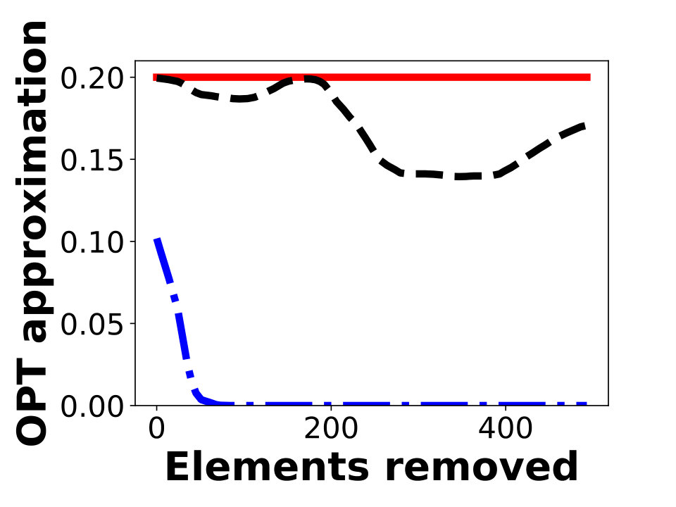 Figure 1
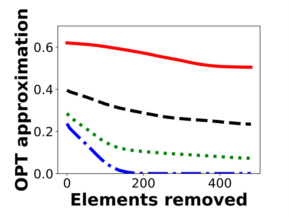 Figure 2
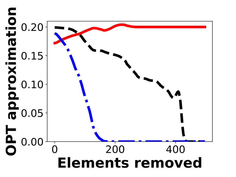 Figure 3
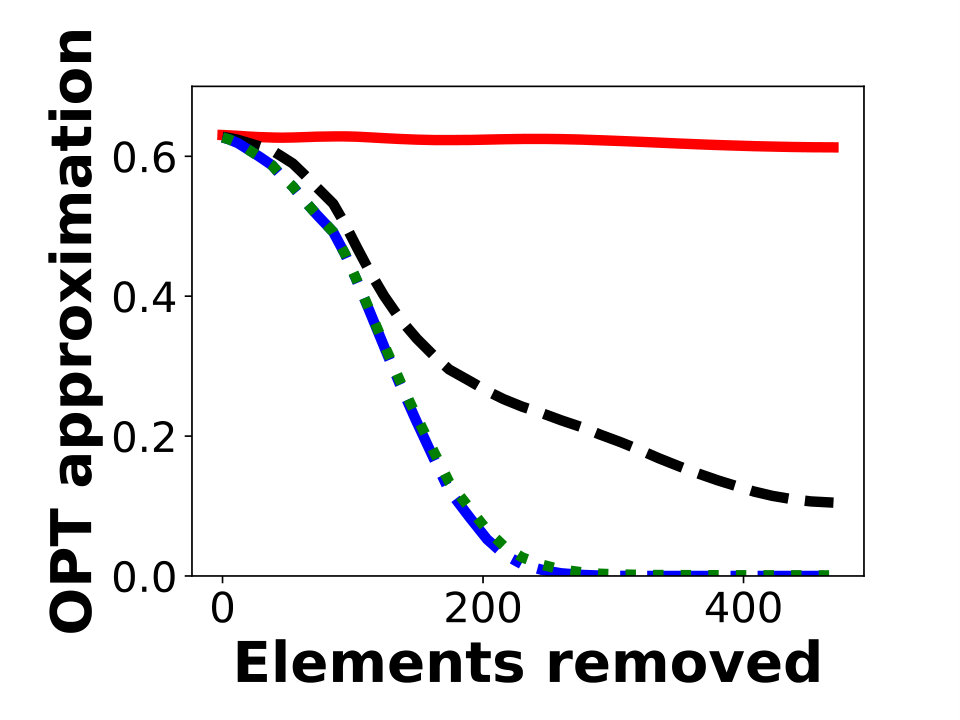 Figure 4
 Figure 5
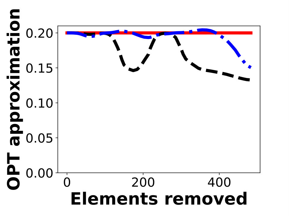 Figure 6
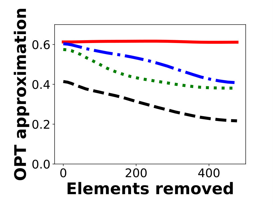 Figure 7
| ml-20, 1 knapsack | fb, 1 knapsack | twitter, 1 knapsack | ml-20, 2 knapsacks | fb, 2 knapsacks | twitter, 2 knapsacks | |
| AlgMult | 641 | 378 | 401 | 1350 | 2745 | 4208 |
| MarginalRatio | 641 | 377 | 402 | 1350 | 2745 | 4209 |
| Multidimensional | 87 | 18 | 435 | 72 | 22 | 4221 |
| Greedy | 647 | 393 | 493 | - | - | - |
Peer Reviews
No public reviews on file for this paper yet. If you reviewed it on a platform where reviews are public (OpenReview, ICLR, NeurIPS, ICML), you can paste yours below so the community can read it here.
Videos
No videos yet. Explain this paper in a talk, walkthrough, or lecture? Add one.
Taxonomy
TopicsComplexity and Algorithms in Graphs · Adversarial Robustness in Machine Learning · Cryptography and Data Security
Adversarially Robust Submodular Maximization under Knapsack Constraints
Dmitrii Avdiukhin Indiana University. E-mail: [email protected]
Slobodan Mitrović MIT. E-mail: [email protected]
Grigory Yaroslavtsev Indiana University & The Alan Turing Institute. E-mail: [email protected]
Samson Zhou Indiana University. E-mail: [email protected]
Abstract
We propose the first adversarially robust algorithm for monotone submodular maximization under single and multiple knapsack constraints with scalable implementations in distributed and streaming settings. For a single knapsack constraint, our algorithm outputs a robust summary of almost optimal (up to polylogarithmic factors) size, from which a constant-factor approximation to the optimal solution can be constructed. For multiple knapsack constraints, our approximation is within a constant-factor of the best known non-robust solution.
We evaluate the performance of our algorithms by comparison to natural robustifications of existing non-robust algorithms under two objectives: 1) dominating set for large social network graphs from Facebook and Twitter collected by the Stanford Network Analysis Project (SNAP), 2) movie recommendations on a dataset from MovieLens. Experimental results show that our algorithms give the best objective for a majority of the inputs and show strong performance even compared to offline algorithms that are given the set of removals in advance.
1 Introduction
Submodular maximization has a wide range of applications in data science, machine learning and optimization, including data summarization, personalized recommendation, feature selection and clustering under various constraints, e.g. budget, diversity, fairness and privacy among others. Constrained submodular optimization has been studied since the seminal work of [32]. It has recently attracted a lot of interest in various large-scale computation settings, including distributed [11, 28], streaming [3, 33, 1], and adaptive [15, 5, 4, 14, 13, 10] due to its applications in recommendation systems [24, 12], exemplar based clustering [16], and document summarization [26, 38, 35]. For monotone functions, constrainted submodular optimization has been studied extensively under numerous constraints such as cardinality [3, 6], knapsack [18], matchings [9], and matroids [8].
With the increase in volume of data, the task of designing low-memory streaming and low-communication distributed algorithms for monotone submodular maximization has received significant attention. A series of results [3, 33, 1] culminated in a single pass algorithm over random-order stream that achieves close to -approximation of monotone submodular maximization under cardinality constraint. This approximation almost matches the guarantee of a celebrated result [32]. Also in the context of streaming, [23, 18, 39] studied monotone submodular maximization under knapsack constraints, resulting in a single pass algorithm that provides -approximation. Another line of work [30, 23, 11, 28] focused on submodular maximization in distributed setting. In particular, [28] developed -round and -round MapReduce algorithms that provide and approximation, respectively, for monotone submodular maximization under cardinality constraint.
In this paper, we focus on the robust version of this classic problem [21, 34, 31, 20]. Consider a situation where a set of recommendations (or advertisements) is constructed for a new user. It is standard to model this as a monotone submodular maximization problem under knapsack constraints, which allow incorporation of various restrictions on available budget, screen space, user preferences, privacy and fairness, etc. However, new users are likely to find some of the recommended items familiar, annoying or otherwise undesirable. Hence, it is advisable to build recommendations in such a way that even if the user later decides to dismiss some of the recommended items, one can quickly compute a new high-quality set of recommended items without solving the entire problem from scratch. We refer to this property as “adversarial robustness” since the removals are allowed to be completely arbitrary (e.g. might depend on the algorithm’s suggestions).
1.1 Adversarially Robust Monotone Submodular Maximization
Let be a finite domain consisting of elements . For a set function , we use to denote the marginal gain of an element given a set , i.e., . A set function is submodular if for every and every it holds that . A set function is monotone if for every it holds that . Intuitively, elements in the universe contribute non-negative utility, but have diminishing gains as the cost of the set increases.
For a set we use notation to denote the 0-1 indicator vector of . We use to denote a matrix with positive entries and to denote a vector with positive entries. Here, C and should be interpreted as knapsack constraints, where set satisfies these constraints if and only if .
Problem 1.1** (MSM under knapsack constraints)**
In the monotone submodular maximization (MSM) problem subject to knapsack constraints, we are given a monotone submodular set function and are required to output:
[TABLE]
Since the constraints are scaling-invariant, one can rescale each row by multiplying it (and the corresponding entry in b) by so that all entries in b are the same and equal to . One can further rescale C and b by the smallest entry in C (or some lower bound on it), so that . We assume such rescaling below and let for all . In the case of one constraint (), we further simplify the notation and set and and refer to simply as the cost of the -th item.
An important role in our algorithms is played by the marginal density of an item. Formally, for a set , an element and a cost function we define the marginal density of with respect to under the cost function as: . For multiple dimensions, we will specifically define the cost function .
Motivated by applications to personalized recommendation systems, we consider the adversarially robust version of the above problem. In the adversarially robust monotone submodular maximization (ARMSM) problem the goal is to produce a small “adversarially robust” summary . Here “adversarial robustness” means that for any set of cardinality at most , which might be later removed, one should be able to compute a good approximation for the residual monotone submodular maximization problem over based only on . In this paper, we propose a study of ARMSM under knapsack constraints:
Problem 1.2** (ARMSM under knapsack constraints)**
An algorithm solves the adversarially robust monotone submodular maximization problem ARMSM subject to knapsack constraints if it produces a summary such that:
[TABLE]
for any set of removals of cardinality at most . gives an -approximation if there exists a set with such that .
The main goal of an adversarially robust algorithm is to minimize the size of the resulting summary. We remark that the above robustness model is very strong. In particular, the set of removals does not have to be fixed in advance and might depend on the summary produced by the algorithm. Hence, we choose to refer to it as adversarial robustness in order to avoid confusion with other notions of robustness known in the literature [2, 36].
1.2 Our Theoretical Results
Streaming algorithms.
We first consider the ARMSM problem in the streaming setting. A streaming algorithm is given the vector b of knapsack budget bounds upfront. Then, the elements of the ground set arrive in an arbitrary order. When an element arrives, the algorithm sees the corresponding column , which lists the costs associated with this item. The algorithm only sees each element once and is required to use only a small amount of space throughout the stream. In the end of the stream, an adversarially chosen set of removals is revealed and the goal is to solve ARMSM over . The key objective of the streaming algorithm is to minimize the amount of space used while providing a good approximation for ARMSM for any .
Our first set of results gives adversarially robust algorithms for the ARMSM problem under one knapsack constraint:
Theorem 1.3** (ARMSM under one knapsack constraint)**
For the ARMSM problem under one knapsack constraint, there exists an algorithm that gives a constant-factor approximation with a summary consisting of elements of the ground set (Theorem 3.1).
We also show that if the total cost of removed items is at most then there is an algorithm with summary size and improved approximation guarantee. For ARMSM under a single knapsack constraint, our bounds are tight up to polylogarithmic factors, since an optimal solution may contain items of unit cost, and an adversary can remove up to items of any set. Hence, storing elements is necessary to obtain a constant factor approximation.
For the ARMSM problem under knapsack constraints, we give an algorithm with the following guarantee:
Theorem 1.4** (ARMSM under knapsack constraints)**
For the ARMSM problem under knapsack constraints, there exists an algorithm that gives an -approximation with a summary of size (Theorem 3.2).
Distributed algorithms.
We also consider the ARMSM problem in the distributed setting. Here, our aim is to collect a robust set of elements while distributing the work to a number of machines, minimizing the memory requirement per machine and the number of rounds in which the machines need to communicate with each other. As in the case of streaming setting, a set of removals is revealed only after is constructed. We obtain a -round algorithm that matches our result for streaming, in terms of approximation guarantees.
Theorem 1.5** (Distributed ARMSM)**
For the ARMSM problem on a dataset of size under knapsack constraints, there exists an algorithm that gives an -approximation with a summary of size . If oracle access to is given, this algorithm can be implemented in two distributed rounds using words of space per machine (Theorem 4.1).
1.3 Empirical Evaluations
We evaluate the performance of our algorithms on both single knapsack and multiple knapsack constraints by comparison to natural generalizations of existing algorithms. We implement the algorithms for the objective of dominating set for large social network graphs from Facebook and Twitter collected by the Stanford Network Analysis Project (SNAP), and for the objective of coverage on a large dataset from MovieLens. We compare the objectives on the sets output as well as the total number of elements collected by each algorithm.
Our results show that our algorithms provide the best objective for a majority of the inputs. In fact, our streaming algorithms perform just as well as the standard offline algorithms, even when the offline algorithms know in advance which elements will be removed. Our results also indicate that the number of elements collected by our algorithms does not appear to correlate with the total number of elements, which is an attractive property for streaming algorithms. In fact, most of the baseline algorithms collect relatively the same number of elements for the robust summary, ensuring fair comparison. For more details, see Section 5.
1.4 Previous Work
The special case of ARMSM with one constraint and equal costs for all elements is referred to as robust submodular maximization under the cardinality constraint. If at most elements can be selected, we refer to this problem as ARMSM. The study of this problem was initiated by Krause et al. [21]. The first (non-streaming) constant-factor approximation for this problem was given by Orlin et al. [34] for . This was further extended by [7] who give algorithms for . In these works, the size of the summary is restricted to contain at most elements and hence by design only removals can be handled.
Recently the focus has shifted to handling larger numbers of removals and so there has been increased interest in studying ARMSM with summary of sizes greater than . [29] solve this problem with summary size , which was improved by [31] to . Moreover, their algorithms are applicable to arbitrary ordered streams. A different setup was considered by [20], who assume that is chosen independently of the choice of a robust summary and give algorithms with summary size , but obtain better approximation guarantees than [31].
To the best of our knowledge, there is little known about the general ARMSM problem considered here which asks for robustness under single or multiple knapsack constraints.
2 Techniques
Our general approach is to find a set at the end of the stream, so that when a set of items is removed, we show that running an offline algorithm, Offline, on the set produces a good approximation to the value of the optimal solution of the entire stream. Since Offline on input is known to produce a good approximation to the optimal solution of constrained submodular maximization on input (see Theorem 2.1), then it suffices to show that is a good approximation to , where we use to denote .
Theorem 2.1
[37, 22]** There exists an algorithm Offline that gives a -approximation for the monotone submodular maximization problem subject to knapsack constraints in polynomial time.
We assume that we have a good guess for by making a number of exponentially increasing guesses . Our algorithms start with the partitions-and-buckets approach from [7, 31] for robust submodular maximization under cardinality constraints. Specifically, our algorithms create a number of partitions and also create a number of buckets for each partition, where the number of buckets is chosen to be “robust” to the removal of items at the end of the stream. An element in the stream is added to the first possible bucket in which its marginal density exceeds a certain threshold, which is governed by the partition. The thresholds are exponentially decreasing across the partitions, so that the number of partitions is logarithmic in .
At a high level, our algorithms overcome several potential pitfalls. The first challenge we face is the issue of buckets being populated with items of small cost whose marginal density surpasses the threshold. These small items prevent large items (such as cost ) whose marginal density also surpasses the threshold from being added to any bucket. If the optimal solution consists of a single large item, then the approximation guarantee could potentially be as bad as . Thus, we allow each bucket double the capacity and create an additional partition level with a smaller threshold to compensate.
The second challenge we face is relating the items in various partitions. Although we would like to argue that an item in a bucket in a certain partition does not have overwhelmingly large marginal gain, the most natural way to prove this would be to claim that would have been placed in a previous partition less than because the ratio is overwhelmingly large. However, this is no longer true because items in partition can have up to cost and any non-empty bucket in previous partitions does not have enough capacity. Surprisingly, for the purposes of analysis, it suffices to prohibit any item in a bucket from using more than a certain fraction of the capacity. That is, any item added to a bucket , which has capacity , must have cost at most .
2.1 Robustness to the Removal of Items
We now describe AlgNum, which outputs a solution of cost on a single knapsack constraint and is robust against the removal of up to items. We would like to use an averaging arguments to show that some “saturated” bucket in a partition cannot have too much intersection with the elements that are removed at the end of the stream. However, the removal of up to items at the end of the stream may cause the removal of cost up to . But then the averaging argument fails unless the number of buckets in each partition also increases by a factor of , which unfortunately gives an additional multiple of in the space of the algorithm.
Instead, the key idea is to dynamically allocate a number of new buckets, depending on the total cost of the current items in the buckets of a partition. The goal is to maintain enough buckets to guarantee that a certain number of elements can be added to a partition, regardless of their cost. Therefore, the number of total buckets is not large unless the stored items have large cost, in which case the number of items is relatively low anyway. To do this, we maintain counters that allocate a new bucket to partition each time they exceed . Each time an item is added to partition , the counter is increased proportional to the cost of the item, . The creation of new buckets is allowed until a certain number of items have been collected by the partition. Intuitively, algorithms robust to the removal of items, such as AlgNum, should strive to output at the end of the stream a set with a certain number of items, whereas algorithms robust to the removal of items with a certain cost should strive to output a set with a certain cost.
At the end, we run a procedure Prune to further bound the number of elements output by the algorithm. Prune simply reorders the elements stored by AlgNum by cost of the elements, and again runs AlgNum on the sorted set of elements as an input stream. Since the items with smaller cost arrive first, this ensures that we cannot have too many items of large cost.
3 Streaming Algorithms
We now warm-up by providing the first streaming algorithm for the ARMSM problem under a single knapsack constraint. We later show how to build on these ideas to obtain robustness subject to multiple knapsack constraints.
3.1 Single Knapsack Constraint
We describe our algorithm AlgNum, which is used to produce a summary consisting of items. Recall that we use to denote . In order to simplify presentation, we assume111This assumption can be removed using standard techniques (see e.g. Appendix E of [31]) by maintaining guesses to find such a . that we have a good estimate for , such that . To simplify presentation, we further assume that is a power of two and hence let (see Algorithm 1 for how rounding is handled).
AlgNum creates partitions where the -th partition initially consists of buckets of capacity each. We refer to the -th bucket in the -th partition as . When processing the stream, each element is added to the first possible bucket in the first possible partition such that the bucket has enough capacity remaining and the marginal density exceeds a certain threshold for this partition. Note that the thresholds exponentially decrease across the partitions while capacities of the buckets exponentially increase.
Our goal is to maintain enough buckets to guarantee that a certain number of elements can be added to a partition, regardless of their cost. To dynamically allocate a number of new buckets, AlgNum keeps counters that create a new bucket while they exceed , after which the value of the counter is lowered. The counter is increased proportional to the cost of an item each time an item is added to partition . This process continues until a certain number of items are in the partition. Finally, we run the procedure Prune to further bound the number of elements output by the algorithm. See Figure 1 for an illustration of the data structure.
By using Prune on the output of AlgNum, we have the following result, whose proof formally appears in Appendix A.
Theorem 3.1
*There exists an algorithm that outputs a set with elements such that, for any set of at most removed items, one can compute from a set with cost at most and is a constant factor approximation to . *
In fact, if the items that are removed has total cost at most , we can provide a better guarantee in terms of both approximation and number of elements stored (see Appendix D).
3.2 Knapsack Constraints
We now consider the ARMSM problem under knapsack constraints. Recall that AlgNum relies on guessing the correct threshold and then using a streaming framework that adds elements whose marginal gain surpasses the threshold. In the case where there are knapsack constraints, a natural approach would be to have parallel instances that guess thresholds for each constraint, and then pick the instance with the best set. This would certainly work, but since there would be guesses for each constraint, the total number of parallel instances would be , which is unacceptable for large values of and . On the other hand, it seems reasonable to believe that the space usage can be improved, at the expense of the approximation guarantee, by maintaining a smaller number of parallel instances. In that case, marginal gain to cost ratio is not well-defined, since there is a separate cost for each knapsack, so what would be the right quantity to consider?
Recall the standard normalization for multiple knapsack constraints discussed in Section 1.1. We define the largest cost of an item to be the maximum cost of the item across all knapsacks, after the normalization. It has been previously shown that the correct quantity to consider for the streaming model is the marginal gain of an item divided by its largest cost [39]. Namely, if the ratio of the marginal gain to the largest cost of an item exceeds the corresponding threshold, and the item fits into a bucket without violating any of the knapsack constraints, then we choose to add the item to the first such bucket. Since the threshold now compares the marginal gain to the largest cost, a natural question to be asked is what quantity should be used for the dynamic allocation of the buckets. Recall that the previous goal of AlgNum was to maintain a specific number of items, so that it would be robust against the removal of items. Thus, we would like to allocate a new bucket for a partition whenever the capacity of the bucket with respect to some knapsack becomes saturated. Hence, AlgMult maintains a series of counters i,a for partition and knapsack , where . Whenever one of these counters exceeds , we create a new bucket entirely in partition , and lower i,a accordingly.
By using Prune on the output of AlgNum, we have the following result, whose proof formally appears in Appendix B. As in Section 3.1, we do not attempt to optimize parameters here, but observe that the number of elements stored is independent of .
Theorem 3.2
*For the ARMSM problem under knapsack constraints, there exists an algorithm that outputs a set of size , from which one can compute a set with cost at most and is a -approximation to . *
4 Distributed Algorithm
In this section, we give a distributed algorithm for the ARMSM problem under knapsack constraints (see Definition 1.2). We use a variant of the MapReduce model of [19], in which we consider an input set of size that is distributed across machines. For some parameters and that are known across all machines, we permit each machine to have memory. The machines communicate to each other in a number of synchronous rounds to perform computation. In each round, each machine receives some input of size , on which the machine performs some local computation. The machine then communicates some output to other machines at the start of the next round. We require that the total input and output message size is per machine. We assume that each machine has access to an oracle that computes . Then our main result in the distributed model is the following.
Theorem 4.1
For the ARMSM problem under knapsack constraints, there exists a two-round distributed algorithm that outputs a set , from which one can compute a set with cost at most and is a -factor approximation to . Moreover, each machine uses space .
The analysis of our distributed algorithm is based on the analysis for our streaming algorithms, along with a recent work by [28]. We generalize their result to obtain a distributed algorithm that constructs a robust summary equivalent to that constructed by AlgMult.
In our algorithm and proofs, we use to denote an upper bound on the number of elements collected by AlgMult. Let be the data structure of sets maintained by AlgMult. We use to refer to the invocation of AlgMult with the following changes:
- •
The buckets are initialized by and the loop on line 6 of AlgMult is ignored.
- •
In place of , the ground set is used.
Our distributed algorithm is explicitly given in Algorithm 6 and uses subroutine PartitionAndSample, which is given in Algorithm 5.
We formally prove Theorem 4.1 in Appendix C by first showing that the approximation guarantee is the same as Theorem 3.2.
Lemma 4.2
There exists a distributed algorithm that outputs a set so that has the same approximation guarantee as stated by Theorem 3.2.
We can also bound the total number of elements sent to the central machine, using a proof similar to [28].
Lemma 4.3
Let be an upper bound on the number of elements collected by AlgMult. With probability , the number of elements sent to the central machine is at most .
5 Experiments
In this section, we provide empirical evaluation of our algorithms for ARMSM under both single knapsack and multiple knapsack constraints. As no prior work exists in this setting we use the most natural generalizations of standard non-robust algorithms for comparison. We test our most general algorithm AlgMult against such algorithms while measuring the number of elements collected and the quality of the resulting approximation. The aim of our evaluations is to address the following points:
How does AlgMult compare to “robustified” generalizations of other submodular maximization algorithms? 2. 2.
How well does AlgMult perform on real datasets compared to our theoretical worst-case guarantees? 3. 3.
How many elements does AlgMult collect? 4. 4.
Does the performance of AlgMult degrade as the number of elements removed at the end of the stream increases?
Implementation is available at https://github.com/KDD2019SubmodularKnapsack/KDD2019SubmodularKnapsack.
Robustification.
Although there are no existing ARMSM algorithms for knapsack constraints, we propose the following modification to existing algorithms to ensure a fair comparison. Given a submodular maximization algorithm , we consider its robustified version by allowing the algorithm to collect extra elements to obtain its own robust summary. To achieve this, we increase the knapsack capacity by some multiplicative factor, which is selected in such way that all algorithms collect approximately the same number of elements.
5.1 Baselines
We compare AlgMult to the following algorithms.
Robustified MarginalRatio.
This algorithm corresponds to a robustified version of Algorithm from [18], which accepts any element whose marginal density with respect to the stored elements exceeds a certain threshold. Note that while the algorithm is for a single knapsack constraint, it can be trivially extended to multiple knapsack constraints by checking that the thresholding condition holds for all dimensions. This marginal density thresholding algorithm is a natural generalization to knapsack constraints of the streaming algorithm Sieve [3] which gives the best theoretical guarantee under the cardinality constraint.
Robustified offline Greedy.
This algorithm builds its summary by iteratively adding to it an element with the largest marginal density. Observe that Greedy is an offline algorithm, which is a more powerful model. However, Greedy is a single knapsack algorithm, so we use it only as a baseline for single knapsack constraints. While there exists a Greedy algorithm [27] under multiple knapsack constraints, it requires running time, which makes it infeasible on large datasets.
Robustified Multidimensional.
This is a robustified version of the streaming algorithm for submodular maximization with multiple knapsack constraints from [39].
5.2 Objectives and Datasets
We evaluate the algorithms on two submodular objective functions:
Dominating set.
We use graphs ego-Facebook (4K vertices, 81K edges) and ego-Twitter (88K vertices, 1.8M edges) from the SNAP database [25]. For a graph and , we let , where is the set of all neighbors of . For each knapsack constraint, the cost of each element is selected uniformly at random from the uniform distribution and all knapsack constraints are set to .
Movie recommendation.
Modeling the scenario of movie recommendations we analyze a dataset of movie ratings (in the range ) assigned by users. For each movie we use a vector of normalized ratings: if user did not rate movie , then set , otherwise set , where denotes the average of all known ratings. Then, the similarity between two movies and can be defined as the dot product of their vectors.
In the case of movie recommendation the goal is to select a representative subset of movies. The domain of our objective is the set of all movies. For a subset of movies we consider a parameterized objective function :
[TABLE]
where is a subset of movies. This captures how representative is of the set . In our experiments, we model the situation of making recommendations to some user so we pick to be a set of movies rated by the user (we select the user uniformly at random). Hence the maximizer of corresponds to a subset of movies which represents well user’s rated set .
We use the ml-20 MovieLens dataset [17], containing movies and ratings. Knapsack constraints model limited demand for movies of a certain type (e.g. not too many action movies, not too many fantasy movies, etc). In the data each movie is labeled by several genres and each knapsack constraint is described by sets of “good” and “bad” genres. Movies with more “good” genres and less “bad” genres have lower cost, allowing the algorithm to choose more such movies. If there are at most genres describing “good” and “bad” sets then we set the cost of a movie to be linear in the range :
[TABLE]
where and are the numbers of good and bad genres that movie is labeled with.
For the experiments under one knapsack constraint, we define the good set of movies as , and the bad set of movies as . For experiments under two knapsack constraints, we define the second constraint by an additional set of good movies , and an additional set of bad movies . All knapsack constraint bounds are set to , limiting the total number of recommended movies.
5.3 Experimental Evaluation and Results
We compare AlgMult against the three baselines described in Section 5.1. First, we obtain robust summaries for AlgMult and for each of the baselines. Second, we adversarially remove elements from these summaries. Finally, we run Offline on the remaining elements in the summaries and compare the values of objective functions on the resulting sets.
Adversarial removals.
To ensure a fair comparison, we use the same set of removed elements for all algorithms. This is done by removing the union of sets recommended by all algorithms and then continuing in a recursive fashion if more removals are required.
We define the removal process formally as follows. For an algorithm , let be the robust summary output by . We let , where the union is taken over all four algorithms tested. That is, is the union of the best elements selected using AlgMult, Greedy, Multidimensional, and MarginalRatio. This typically already gives a good choice of removals. If more removals are required, we define . That is, we recursively remove the union of the elements in the optimal sets across all the algorithms and we repeat this process until is empty.
Evaluation.
For different numbers of removed elements, we compare the values that are produced by the offline algorithm on robust summaries, i.e. generated by the four algorithms. Since is NP-hard to compute, we compare the performance of each algorithm with upper bounds on to estimate the approximation given by the algorithms. For a single knapsack constraint, the best known upper bound can be computed from Greedy and for multiple knapsack constraints from Multidimensional [39].
Results.
The results of our experiments are shown in Figure 2. For each algorithm, we plot the ratio of its objective to an upper bound on the optimal solution, which is obtained as previously discussed. Figures 2a, 2b, and 2c show experimental results for -knapsack constraints using Greedy as the offline algorithm with approximation factor , where is the knapsack constraint and is the cost of the resulting set. For many instances, is close to , so this value is close to . Figures 2d, 2e, and 2f show experimental results for -knapsack constraints.
Our evaluations suggest that AlgMult provides the best possible approximation factor for a majority of inputs. Except for the first iterations in Figure 2d, AlgMult outperforms the other algorithms, and achieves roughly the same approximation guarantee as the offline algorithm that knows the items to be removed in advance. In fact, the advantage of AlgMult becomes more noticeable as larger numbers of elements are removed.
Since the baseline algorithms, other than Greedy, require an estimate of , we try several such estimations. The non-monotone behavior of the ratio of MarginalRatio to in Figure 2f occurs since MarginalRatio performs better when estimation is close to the true objective. We emphasize the fact that all algorithms, including AlgMult, use the same estimations. It is possible to obtain a more monotone behavior by trying more estimations, but doing so will require collecting more elements.
To evaluate memory consumption, we also report the number of elements collected by each algorithm. These results are presented in Table 1 and show that the algorithms for -knapsack constraints collect noticeably more elements than those performing maximization under a single knapsack constraint. The size of the robust summary output by AlgMult does not appear to correlate with the total number of elements, and in the case of ego-Twitter, it collects only of the vertices.
Recall that we allow the baseline algorithms to collect extra elements by increasing their knapsack capacity to ensure fair comparison. Hence, almost all the algorithms collect similar numbers of elements for each setup, as shown in Table 1. Note that, however, for some experimental setups Multidimensional collects significantly fewer elements than the other algorithms. This phenomenon persists even if the knapsack capacity is unbounded.
In our empirical evaluations, the number of collected elements did not seem to depend on the number of removed items . One possible reason for this phenomena is that the algorithms were not executed with small guesses for the optimal objective. As a result when the number of removed elements is large, the optimal objective is below the threshold considered by the algorithm, and therefore more elements are not collected because the threshold is set to be too high. However, it is natural that with sufficiently bad guesses for the optimal objective, any thresholding algorithm will be forced to meaninglessly collect a large number of elements.
6 Conclusion
We have given the first streaming and distributed algorithms for adversarially robust monotone submodular maximization subject to single and multiple knapsack constraints. Our algorithms are based on a novel data structure which dynamically allocates new space depending on the elements stored so far and perform well on large scale data sets, even compared to offline algorithms that know in advance which elements will be removed.
For the future work, it is natural to ask whether our framework can be scaled to larger datasets for some specific classes of objectives, e.g., is it possible to ensure adversarial robustness with sketching methods for coverage objectives [6]? It would be also interesting to understand the limits on approximation that can be achieved with adversarial robustness and summary size only . Finally, an interesting open question is whether it is possible to do adversarially robust non-monotone submodular maximization.
Appendix A Missing Proofs from Section 3.1
We call a bucket saturated if the cost of its items is at least half of its capacity.
Definition A.1
A bucket , is saturated if .
We break the analysis into the following three cases:
At least half of the buckets in some partition are saturated (Lemma A.2) 2. 2.
More than half of the buckets in all partitions are not saturated, but there exists some bucket in the last partition which is a good estimate of (Lemma A.7) 3. 3.
More than half of the buckets in all partitions are not saturated and no bucket in the last partition is a good estimate of (Lemma A.8)
We first show that if at least half of the buckets in some partition are saturated, some saturated bucket in this partition cannot be affected too much by the removal of elements at the end of the stream. Hence, this saturated bucket contains a set of elements such that is a good approximation to , which in turn is a good approximation to .
Let denote the data structure output by AlgNum when run with parameter (i.e. for ). Let .
Lemma A.2
Let and . If there exists a partition in with at least half of its buckets saturated, then for the set it holds that:
[TABLE]
**Proof : ** Let be a partition in with at least half of its buckets saturated. Let be a saturated bucket that minimizes the cost of removed items, i.e. , among all saturated buckets in this partition. Let be the cost all items in which are in partition , i.e. . Then the total capacity of all buckets in partition is at least . Thus, the total number of buckets in partition is at least . Since at least half of its buckets are saturated the total number of the saturated buckets in partition is at least . By an averaging argument:
[TABLE]
Thus, . Since is saturated by definition, then , and hence the marginal density of each element exceeds a threshold of so that:
[TABLE]
Hence by Theorem 2.1, running Offline on gives value at least .
Before considering the other cases, we need the following technical lemmas. Lemma A.3 bounds the value of the removed elements, while Lemma A.4 allows us to relate the elements removed in a bucket of the last partition with the elements removed in previous partitions.
Lemma A.3
Given a bucket from partition that is not saturated, then the loss in bucket induced by the removals is at most
[TABLE]
where denotes the elements that are removed from .
**Proof : ** By submodularity,
[TABLE]
For each , either or . In the first case, . In the second case, since it must hold that . On the other hand, but because is not saturated. Thus, or else the algorithm would have added to . Hence, for all and so by Equation 1, .
Lemma A.4
Suppose that there exists some bucket in every partition that is not saturated. Let . For every partition , let denote a bucket with and let denote the elements that are removed from . The loss in the bucket induced by the removals, given the remaining elements in the previous buckets, is at most
[TABLE]
**Proof : ** We show by induction that for any the following holds
[TABLE]
so that the claim by setting by setting .
Base case .
Since and each item is normalized to have cost at least , it follows that both and are empty. Thus
[TABLE]
where the first inequality holds by Lemma A.3.
Inductive step .
Assuming Equation 2 holds for where , we now show that it also holds for . By submodularity, . It follows that , by adding to both sides. Since and are disjoint, then
[TABLE]
We can bound the first term by at most , by monotonicity. Note that the third term equals , which is at least , because .
Hence, Equation A gives is at most the sum . Then by submodularity, is at most the sum . Since , Lemma A.3 implies . By the inductive hypothesis, .
We require the following structural lemma from [31].
Lemma A.5
[31]** For any monotone, non-negative submodular function on a ground set , and any sets , we have
[TABLE]
We also require the following structural lemma relating sets of large size to a large number of sets of small size.
Lemma A.6
Let be a set of size for some integer such that no item in has size more than . Then the items of can be partitioned into sets, each with size at most .
**Proof : ** Let be sets that partition with the minimal cardinality . Note that , or else the elements of set and can be combined into a single set, contradicting the definition of . Similarly, for each integer . On the other hand, , so and there can be at most sets.
We can finally consider the second case of our analysis, where more than half of the buckets in all partitions are not saturated, but there exists some bucket in the last partition such that is a good estimate of .
Lemma A.7
Let and . If no partition in has at least half of its buckets saturated, then:
[TABLE]
where is any bucket in the last partition that is not saturated.
**Proof : ** Let and let be the bucket in partition with that minimizes . We denote . By setting , and in Lemma A.5, it follows that f\left(\bigcup_{i=0}^{\ell}(A_{i}\setminus E_{i})\right)\geq f\left(B_{\ell,{r}}\right)-f\left(E_{\ell}\bigg{|}\bigcup_{i=0}^{\ell-1}(A_{i}\setminus E_{i})\right). Hence, applying Lemma A.4 with the observation that each , then
[TABLE]
Let denote the subset of that intersects buckets of partition . For the sake of presentation, we denote . Then the total space in partition is at least . Similarly, the number of buckets in partition is at least , of which at least half are not saturated. Since is defined to be the bucket of partition that minimizes among all the buckets that are not saturated, then by an averaging argument
[TABLE]
Therefore,
[TABLE]
Define for . Then . Hence,
[TABLE]
Note that since , then . Moreover, defining the function by , where , we see that is concave. Thus by Jensen’s inequality and setting , it follows that . Since , then
[TABLE]
Plugging Equation 5 and Equation 6 into Equation 4,
[TABLE]
We can also bound the cost of the elements in : . Hence, the optimal value of on on a set of cost , which we denote , is at least . By Lemma A.6, any set with size whose items have size at most can be partitioned into sets, each with size at most . Therefore by Theorem 2.1, . By submodularity, and thus, .
Finally, in the third case of our analysis, where more than half of the buckets in all partitions are not saturated and no bucket in the last partition produces a value that is a good estimate of .
Lemma A.8
Let and . If no partition in has at least half of its buckets saturated, then:
[TABLE]
where is any bucket in the last partition that is not saturated.
**Proof : ** Let be the set that contains all elements from that are buckets in with higher priority than and let . For each ,
[TABLE]
due to the fact that is the bucket in the last partition and is not saturated.
Since , then by submodularity, . Then by monotonicity, . By submodularity, . Then by Equation 7, . Since , then
[TABLE]
Therefore, by Theorem 2.1, . Since , then . The capacity of is at most , so . Hence by Equation 8, , as desired.
Since the above three lemmas hold for every we can pick its value to give the desired approximation guarantee and space complexity bound. This gives Theorem 3.1, which corresponds to the first part of Theorem 1.3.
Theorem A.9
Let and . There exists an algorithm that outputs a set with elements such that, for any set of at most removed items, one can compute from a set with cost at most and
[TABLE]
**Proof : ** Fix any value of and consider the bounds of Lemma A.7 and Lemma A.8 as functions of . Note that the first bound increases and the second bound decreases as a function of this parameter. Since we can always pick the better bound, the worst value for is when the two bounds are equal, i.e. . This occurs when . Hence, the best of these two bounds is always at least .
Note that this is a decreasing function of while the inequality of Lemma A.2 is an increasing function of , so we pick to make sure that the minimum of these two bounds is large. The optimal value of is in which case the two bounds are equal. Hence, . By making guesses for by increasing powers of , we can obtain a approximation of , giving a approximation for .
Finally, we give the bound on the number of elements returned. The number of buckets is dynamically updated until . Hence at most new buckets have been created for partition . Then the total number of elements in each partition is at most since . Since there are partitions, the total number of elements is for each guess of . Assuming , then the total number of guesses for is , so the total number of elements is .
We now show that Prune reduces the total number of elements output, while maintaining a constant factor approximation.
Lemma A.10
Suppose AlgNum outputs a set from which one can compute a set with cost at most and is an -approximation to . Then Prune outputs a set of size , from which one can compute a set with cost at most and is an -approximation to .
**Proof : ** Since Prune runs an instance of AlgNum on , then Prune provides an -approximation to , which is an -approximation to . Thus, is an -approximation to .
It remains to bound the number of elements in . Consider the state of AlgNum on the set sorted by size. Note that no new buckets are created in partition when the total number of items in the bucket is . Let be the first time at which partition contains items, and let all the elements placed in partition before time be called “old” while all the elements that are placed in partition after time be called “new”. Observe that each old element increments by a multiple of its cost. Since each new element costs at least as much as each old element, new elements will cost at least times the cost of the old elements, which fills the additional space allocated by the old elements.
Hence, the total number of elements in each partition is at most since . Since there are partitions, the total number of elements for each guess of is . Assuming , then the total number of guesses for is , so the total number of elements is .
Together, Theorem A.9 and Lemma A.10 give the proof of Theorem 3.1. A similar approach can be used to prove Theorem 3.2.
Appendix B Missing Proofs from Section 3.2
For a specific knapsack , we call a bucket saturated with respect to knapsack if . As before, we use to denote the data structure output by AlgNum when run with parameter (i.e. for and , where is the set of elements that are removed at the end of the stream. Finally, recall that .
Lemma B.1
Let . For a fixed knapsack , if there exists a partition in with at least half of its buckets saturated with respect to knapsack , then
[TABLE]
**Proof : ** Let be a fixed knapsack and be a partition in with at least half of its buckets saturated with respect to knapsack . Let be a saturated bucket that minimizes . Let be the cost of the items of with respect to knapsack that are in partition ,
[TABLE]
Then the total space in partition is at least , so the total number of buckets is at least . Since at least half of its buckets are saturated with respect to knapsack , the total number of saturated buckets is at least
By an averaging argument, the cost of the elements in with respect to knapsack that are removed by is at most
[TABLE]
Thus, is at least .
Note that if is saturated with respect to knapsack , then the marginal density of each element exceeds a threshold of so that . Since and for a saturated bucket , then it follows that . Hence by Theorem 2.1, running Offline on produces a approximation.
The following lemma corresponds to Lemma A.3, using the threshold of AlgMult.
Lemma B.2
Let denote the elements that are removed from a bucket in partition . Given a bucket from partition that is not saturated and any knapsack , then the loss in bucket induced by the removals is at most
[TABLE]
The following lemma corresponds to Lemma A.4, using Lemma B.2 and the threshold of AlgMult.
Lemma B.3
Suppose that there exists some bucket in every partition that is not saturated with respect to some particular knapsack . For every partition , let denote a bucket with and let denote the elements that are removed from . The loss in the bucket induced by the removals, given the remaining elements in the previous buckets, is at most .
The following lemma corresponds to Lemma A.7, using Lemma B.3, the threshold of AlgMult, and the observation that an optimal solution considering only a particular knapsack constraint is at least as good as an optimal solution considering additional other knapsack constraints. However, the factor in the denominator results from a bucket , due to the definition of .
Lemma B.4
Let . If no partition in has at least half of its buckets saturated with respect to any knapsack with , then , where is any bucket in the last partition that is not saturated.
The following lemma is similar to Lemma A.8 and follows along the same proof, with the observation that .
Lemma B.5
Let . If no partition in has at least half of its buckets saturated with respect to any knapsack with , then , where is any bucket in the last partition that is not saturated.
We now prove Theorem 3.2.
**Proof of Theorem 3.2: ** The -approximation guarantee follows from Lemma B.1, Lemma B.4 and Lemma B.5, when , and . The -approximation guarantee and space bounds follow from Lemma A.10 with Prune using AlgMult instead of AlgNum.
Appendix C Missing Proofs from Section 4
We first prove Lemma 4.2.
**Proof of Lemma 4.2: ** We will show that returned by line 14 of Algorithm 6 equals to the output of AlgMult run on a stream of such that:
- •
is a prefix of this stream.
- •
Elements of appear in the same order in the stream as they appear in Algorithm 6.
- •
The order of the remaining elements is arbitrary.
Let be the structure of sets and their content after AlgMult is executed on this stream.
Next, recall that AlgMult never removes any element from any . Also, recall that is obtained by executing AlgMult on . Hence, since is a prefix of the stream, for each the content of in is a subset of the content of in . Furthermore, is a submodular function, so if an element is not added to due to its small marginal gain, will not be added to a superset of neither. This implies that after is processed, no element that is not added to on line 8 of Algorithm 6 can ever be added to any (regardless of ordering of the elements ). Therefore, the only relevant elements in the rest of the stream are those in .
The proof now follows from the fact that Theorem 3.2 holds regardless of ordering of the stream.
To prove Lemma 4.3, we need the following result for submartingales.
Theorem C.1** (Azuma’s Inequality)**
Suppose is a submartingale and . Then
[TABLE]
**Proof of Lemma 4.3: ** Observe that the expected number of elements in is so that occurs only with probability at most by standard Chernoff bounds. Thus, with high probability. Let denote the total number of elements that are added to by , so that exactly elements are sent to in round two.
Suppose we split the sample set into pieces of size and process each piece sequentially. Suppose further that before some piece, there are at least remaining elements that would be added to as described above. Then an additional element is added to with probability at least , conditioned on any previous actions of the algorithm, since each piece can be sampled independently and thus we can use a martingale argument to bound the number of elements selected in .
Let be the indicator random variable for the event that at least one element is selected from the -th piece so that . Let so that the sequence is a submartingale and hence, and . Therefore, by Azuma’s inequality (Theorem C.1). Hence with probability , and includes at least elements overall, in which case nothing is sent to the central machine. Otherwise, the number of remaining elements added to is less than .
Appendix D Robust to removal of size
In this section, we consider the ARMSM problem under a single knapsack constraint, when the items have cost at most . In contrast to AlgNum, we no longer need a dynamic allocation of new buckets, so having a fixed number of buckets for each partition suffices. We give our algorithm in full in AlgSize.
To show that the optimal solution of output by AlgSize is a good approximation to the optimal solution of the entire stream, we call a bucket saturated if and break the analysis into the following three cases:
At least half of the buckets in some partition are saturated (Lemma D.1) 2. 2.
More than half of the buckets in all partitions are not saturated, but there exists some bucket in the last partition that is a good estimate of (Lemma D.2) 3. 3.
More than half of the buckets in all partitions are not saturated and no bucket in the last partition is a good estimate of (Lemma D.3)
In the first case, if most of the buckets in some partition are saturated, we argue through an averaging argument that some saturated bucket in this partition cannot have too much size intersection with the elements that are removed at the end of the stream, giving a lower bound on . Since elements can only be added to this bucket if the ratio of their marginal gain to their size exceeds a certain threshold, then we conclude that is at least the product of this threshold, which gives a good approximation to .
In the second case, if there exists some bucket in the last partition that is a good estimate of , we first use a technical lemma to show that the optimal solution on is at least minus the value of the elements across all the buckets that were deleted by . To bound the value of these elements, we argue that if most of the buckets in all partitions are not saturated, then no element in a bucket that is deleted by can value that is too high, because otherwise it would have been added to a bucket in some previous partition less than . Hence, we derive an upper bound on the value of the elements across all the buckets that were deleted by , and this suffices to show that the optimal solution of is close to , since is a good approximation to .
In the third case, if all buckets in the last partition give poor estimates of , then for each of these buckets, the total size of the elements in the bucket cannot be large. As a result, most elements of must either be in a previous partition or have poor marginal gain. If most elements of are in a previous partition, then the union of the items in the previous partitions are contained in and thus the optimal solution of is a good approximation to . If most elements of have poor marginal gain, then there must be some item of with substantial value. On the other hand, since each partition contain many buckets that are not saturated, then this substantial item must have been captured by some bucket in a previous partition and so again, the optimal solution of is a good approximation to . Intuitively, if at least half of the buckets in some partition are saturated, then some saturated bucket in this partition cannot be affected too much by the removal of elements at the end of the stream. Hence, this bucket gives a good approximation to , which in turn serves as a good approximation to .
Lemma D.1
Let . If there exists a partition in such that at least half of its buckets are saturated, then
[TABLE]
**Proof : ** Let be a partition such that half of its buckets are saturated. Let be a saturated bucket that minimizes . Since every partition contains buckets, the number of saturated buckets in partition is at least . By a simple averaging argument and the observation that ,
[TABLE]
Thus,
[TABLE]
Note that if is saturated, then the marginal gain to weight ratio of each element exceeds a threshold of so that
[TABLE]
where the last step follows from the observation that for a saturated bucket . Hence, running Offline on produces a approximation by Theorem 2.1.
The second case of our analysis occurs when more than half of the buckets in all partitions are not saturated, but there exists some bucket in the last partition that is a good estimate of . We now show that AlgSize yields a good approximation in this case.
Lemma D.2
Let and . If no partition in has at least half of its buckets saturated, then
[TABLE]
where is any bucket in the last partition that is not saturated.
**Proof : ** Let . Let denote the bucket in partition with for which is minimized, where . By setting , and in Lemma A.5, we have that f\left(\bigcup_{i=0}^{\ell}(B_{i}\setminus E_{i})\right)\geq f\left(B_{\ell,{r}}\right)-f\left(E_{\ell}\bigg{|}\bigcup_{i=0}^{\ell-1}(B_{i}\setminus E_{i})\right). Since each , then by Lemma A.4, is at least
[TABLE]
Let denote the subset of that intersects buckets of partition . Since each is defined to be the bucket of partition that minimizes among all the buckets that are not saturated and each partition contains buckets, of which more than half are not saturated, then is at most
[TABLE]
Hence,
[TABLE]
Plugging this inequality into Equation 9,
[TABLE]
The cost of the elements in is at most . Hence, the optimal value of on on a set of cost , which we denote , is at least . Therefore,
[TABLE]
where the first inequality holds by Theorem 2.1 and the second inequality holds by submodularity and the observation that any set with size whose items have size at most can be partitioned into sets, each with size at most (i.e., Lemma A.6).
The following lemma is the same as Lemma A.8, with the identical proof.
Lemma D.3
Let and . If no partition in has at least half of its buckets saturated, then
[TABLE]
where is any bucket in the last partition that is not saturated.
Theorem D.4 then follows from optimizing parameters to give an approximation guarantee for an algorithm using AlgSize, when the items have cost at most .
Theorem D.4
*For the ARMSM problem subject to a knapsack constraint, there exists an algorithm that outputs a set so that is a constant factor approximation to and stores elements, if the removed items have cost at most . *
**Proof : ** Let and . Let . From Lemma D.2 and Lemma D.3, it follows that the worst case bound for occurs when . Some straightforward computation shows this occurs when . It follows from Lemma D.1 that the optimal value of occurs at , which gives . For , we have , so . By making guesses for by increasing powers of , we can obtain a approximation of , giving a approximation for .
Allowing each element in to be stored by AlgSize using one word of space, then the total space that AlgSize uses is at most
[TABLE]
Since , then . Assuming , then the total number of guesses for is . Therefore, the total number of stored elements is .
The reference list from the paper itself. Each links out to its DOI / PubMed record.
- 1[1] Shipra Agrawal, Mohammad Shadravan, and Cliff Stein. Submodular secretary problem with shortlists. ar Xiv preprint ar Xiv:1809.05082 , 2018.
- 2[2] Nima Anari, Nika Haghtalab, Joseph Naor, Sebastian Pokutta, Mohit Singh, and Alfredo Torrico. Robust submodular maximization: Offline and online algorithms. Co RR , abs/1710.04740, 2017.
- 3[3] Ashwinkumar Badanidiyuru, Baharan Mirzasoleiman, Amin Karbasi, and Andreas Krause. Streaming submodular maximization: Massive data summarization on the fly. In Proceedings of the 20th ACM SIGKDD international conference on Knowledge discovery and data mining , pages 671–680. ACM, 2014.
- 4[4] Eric Balkanski, Aviad Rubinstein, and Yaron Singer. An exponential speedup in parallel running time for submodular maximization without loss in approximation. In Proceedings of the Thirtieth Annual ACM-SIAM Symposium on Discrete Algorithms, SODA , pages 283–302, 2019.
- 5[5] Eric Balkanski and Yaron Singer. The adaptive complexity of maximizing a submodular function. In Proceedings of the 50th Annual ACM SIGACT Symposium on Theory of Computing, STOC , pages 1138–1151, 2018.
- 6[6] Mohammad Hossein Bateni, Hossein Esfandiari, and Vahab S. Mirrokni. Optimal distributed submodular optimization via sketching. In Proceedings of the 24th ACM SIGKDD International Conference on Knowledge Discovery & Data Mining, KDD , pages 1138–1147, 2018.
- 7[7] Ilija Bogunovic, Slobodan Mitrović, Jonathan Scarlett, and Volkan Cevher. Robust submodular maximization: A non-uniform partitioning approach. In Proceedings of the 34th International Conference on Machine Learning, ICML , pages 508–516, 2017.
- 8[8] Gruia Călinescu, Chandra Chekuri, Martin Pál, and Jan Vondrák. Maximizing a monotone submodular function subject to a matroid constraint. SIAM J. Comput. , 40(6):1740–1766, 2011.