TL;DR
This paper introduces a novel adversarial variational embedding framework that combines VAE and GAN to improve semi-supervised learning by producing exclusive latent codes and meaningful data generation.
Contribution
It proposes AVAE, a new framework that leverages VAE++ and GAN to enhance semi-supervised classification with more exclusive latent representations and better data generation control.
Findings
Outperforms state-of-the-art semi-supervised models on four real-world datasets.
Produces more exclusive and meaningful latent codes for classification.
Enhances the quality and control of generated data.
Abstract
Semi-supervised learning is sought for leveraging the unlabelled data when labelled data is difficult or expensive to acquire. Deep generative models (e.g., Variational Autoencoder (VAE)) and semisupervised Generative Adversarial Networks (GANs) have recently shown promising performance in semi-supervised classification for the excellent discriminative representing ability. However, the latent code learned by the traditional VAE is not exclusive (repeatable) for a specific input sample, which prevents it from excellent classification performance. In particular, the learned latent representation depends on a non-exclusive component which is stochastically sampled from the prior distribution. Moreover, the semi-supervised GAN models generate data from pre-defined distribution (e.g., Gaussian noises) which is independent of the input data distribution and may obstruct the convergence and…
Click any figure to enlarge with its caption.
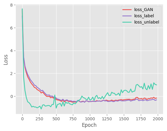 Figure 1
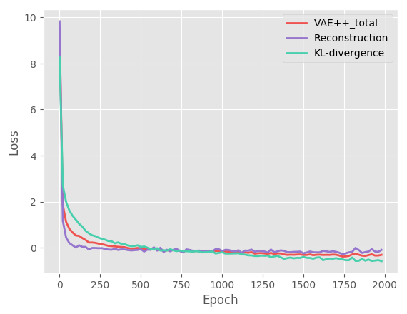 Figure 2
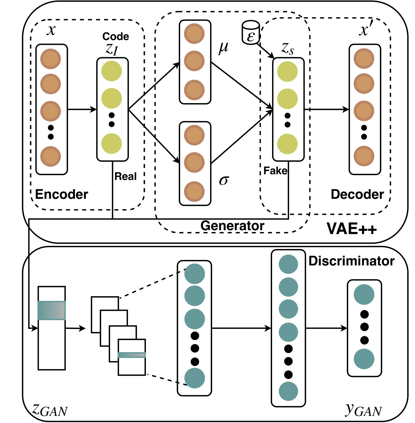 Figure 3
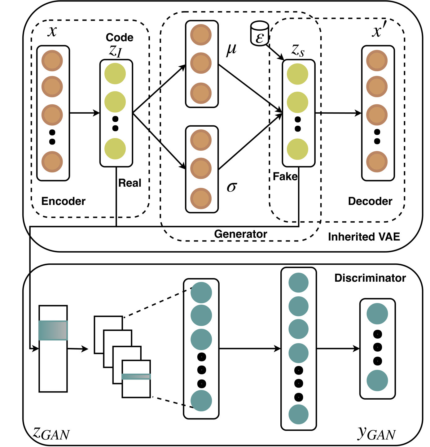 Figure 4
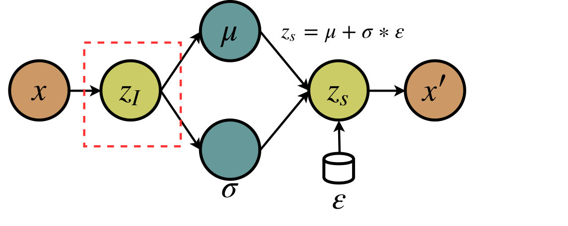 Figure 5
 Figure 6
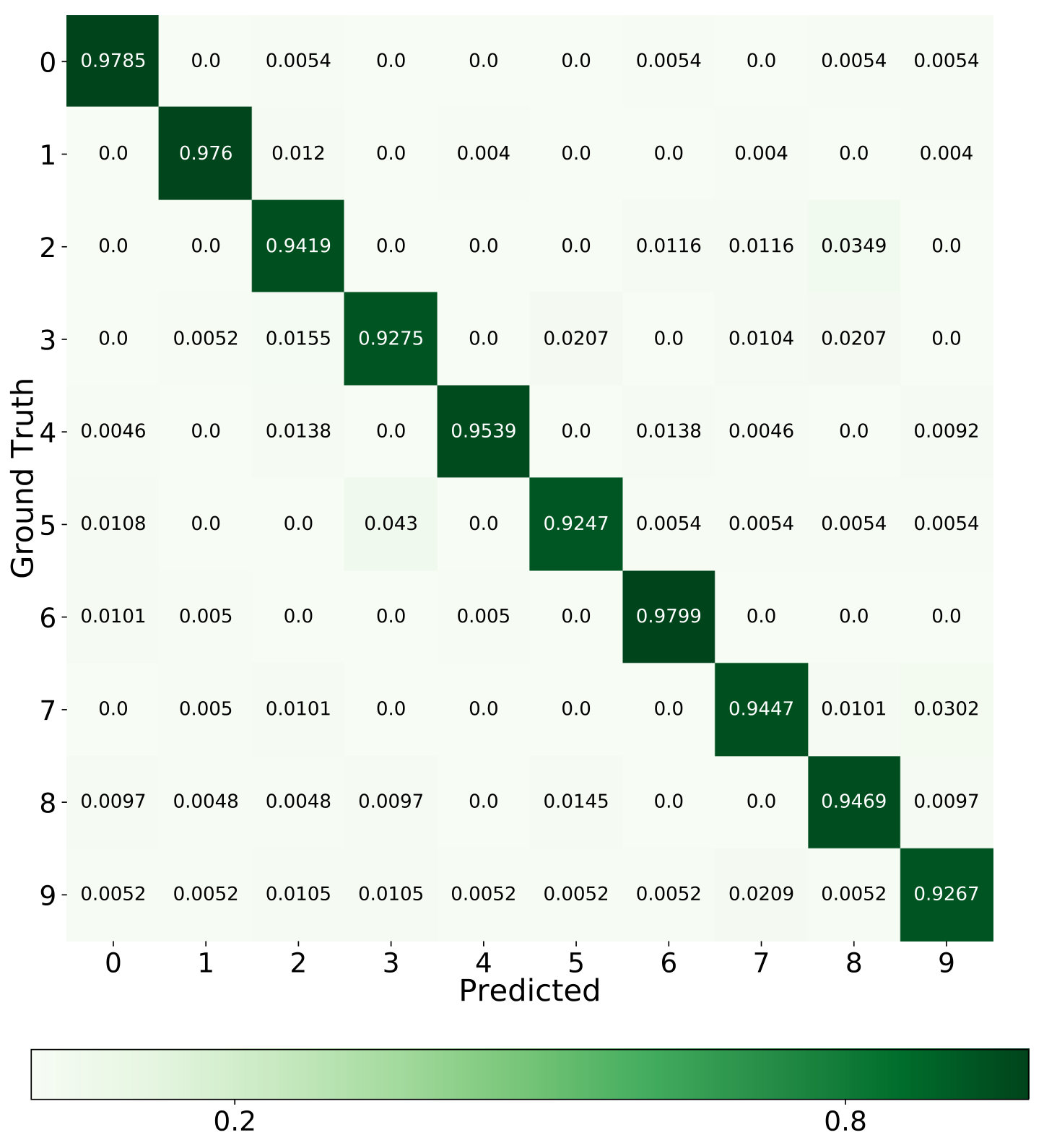 Figure 7
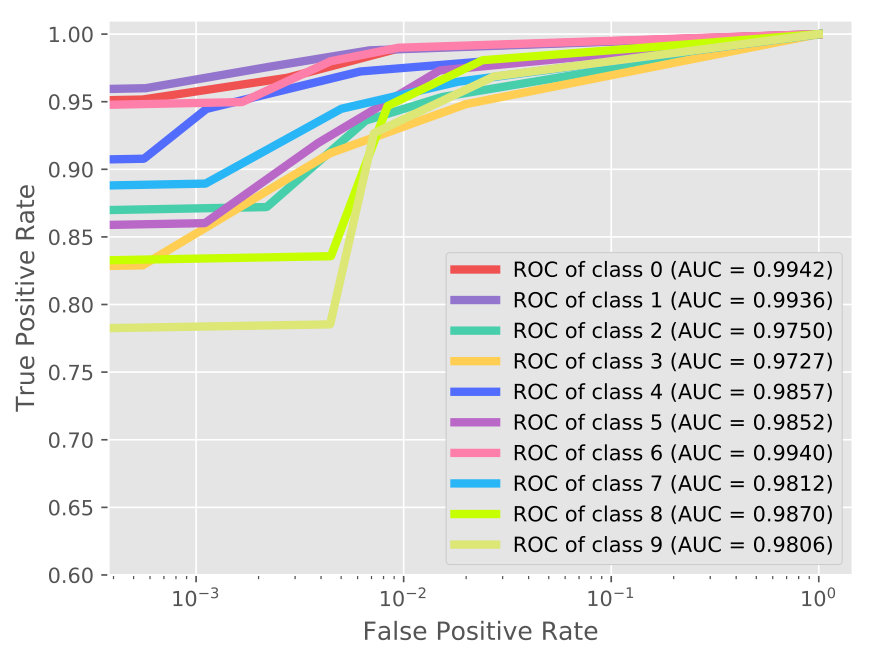 Figure 8
 Figure 9
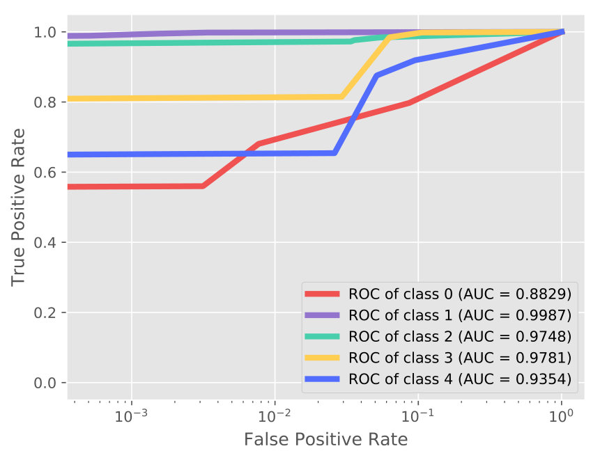 Figure 10
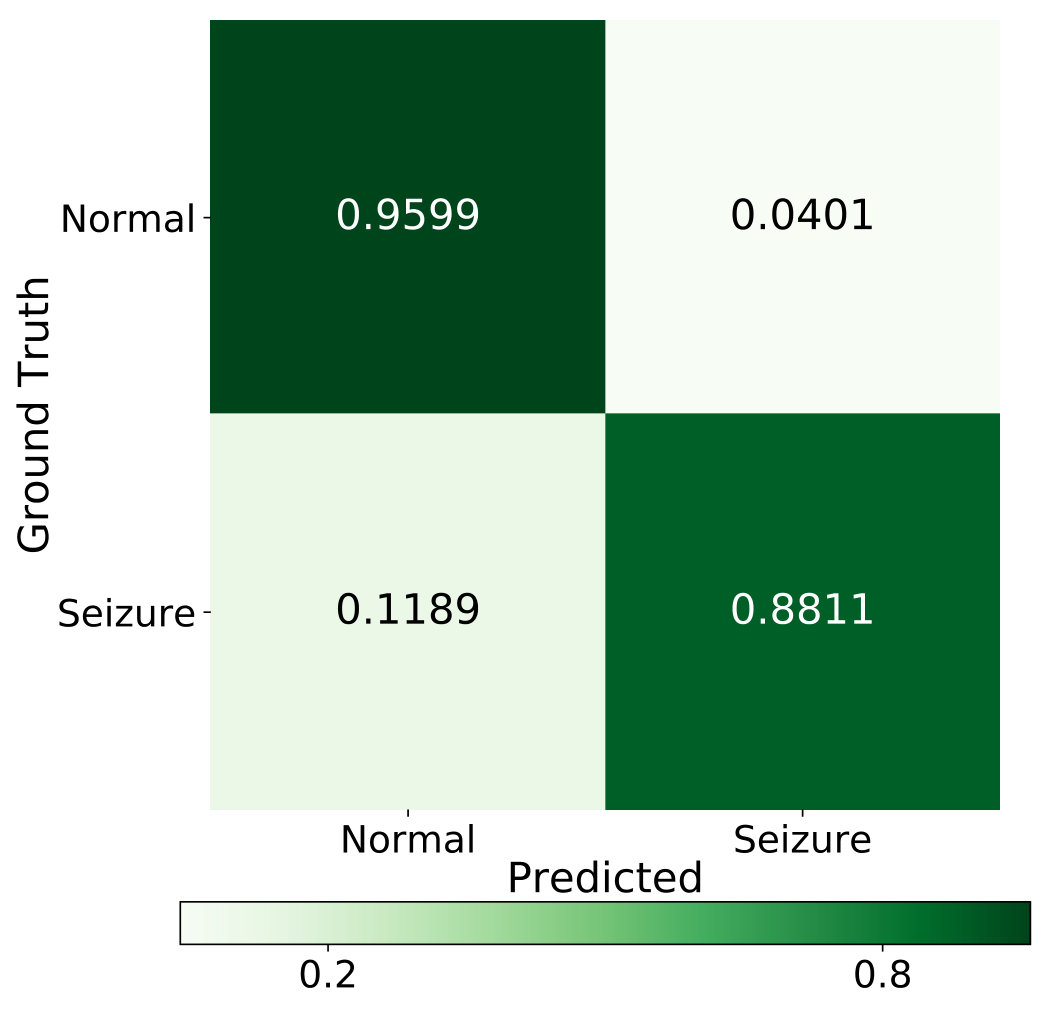 Figure 11
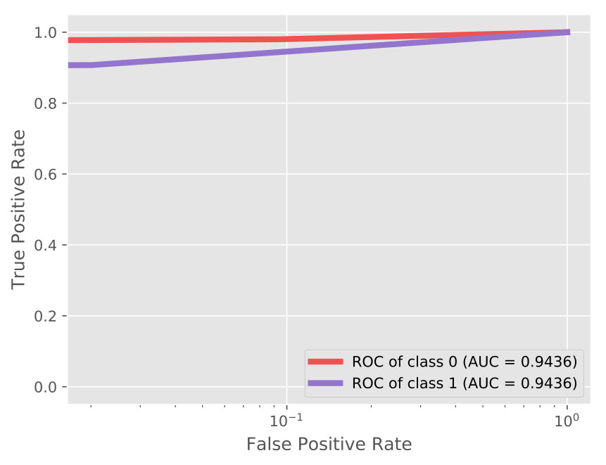 Figure 12
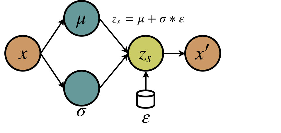 Figure 13
 Figure 14
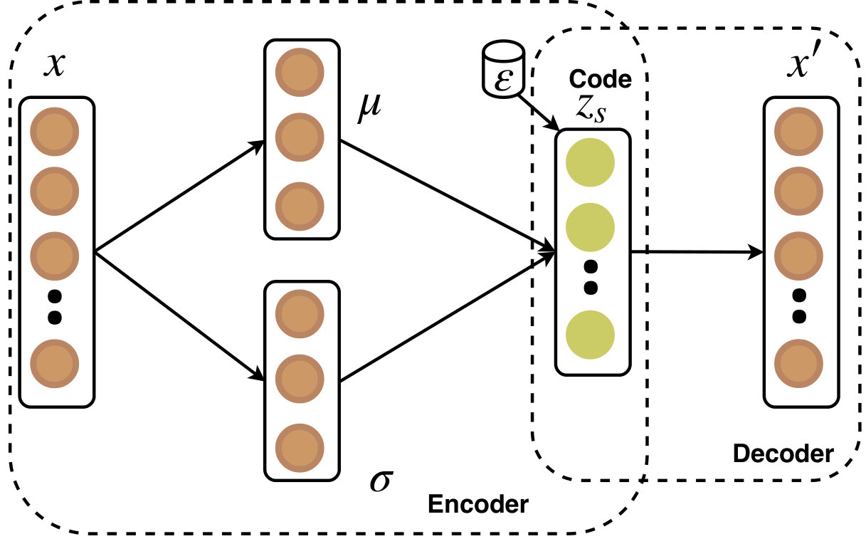 Figure 15
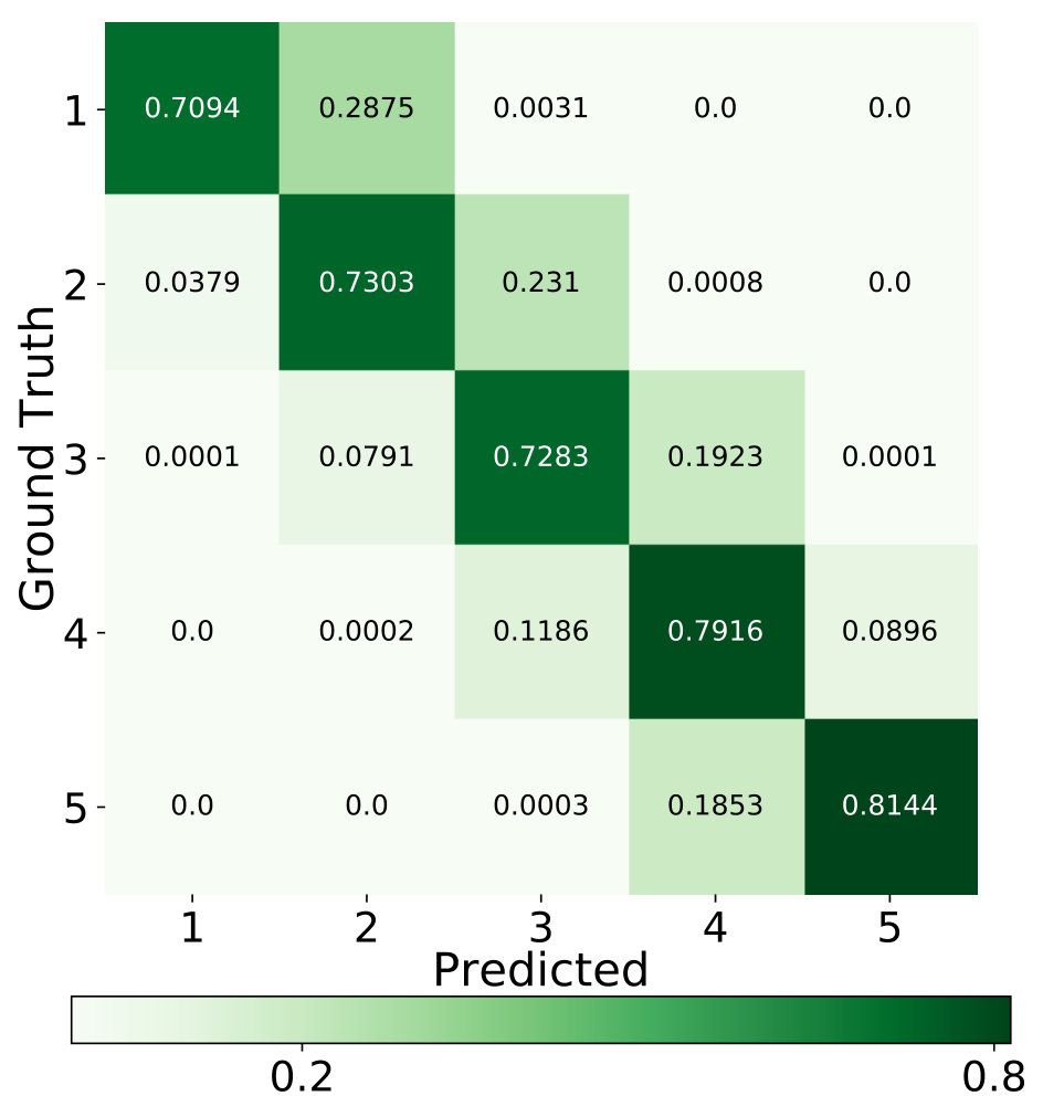 Figure 16
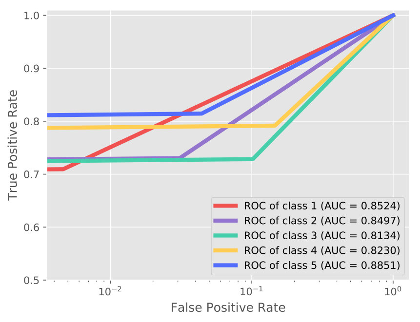 Figure 17
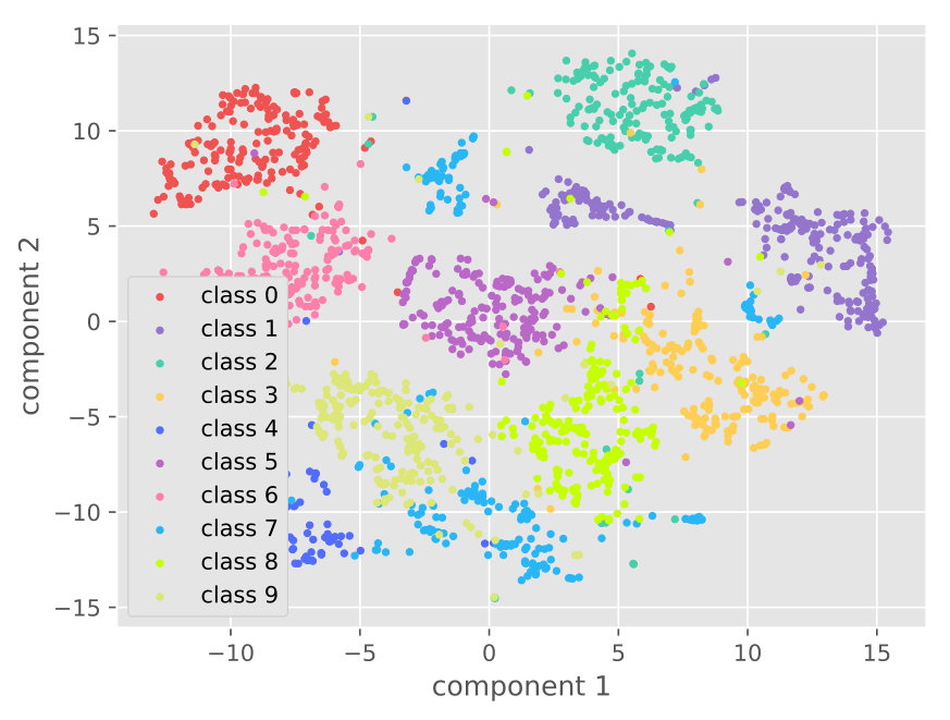 Figure 18
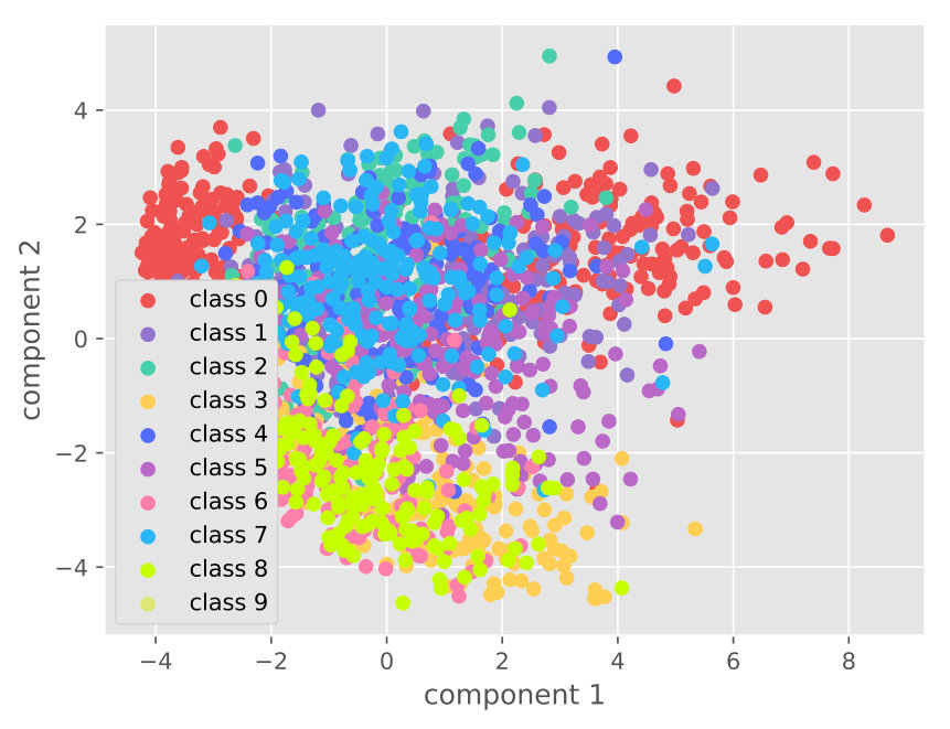 Figure 19
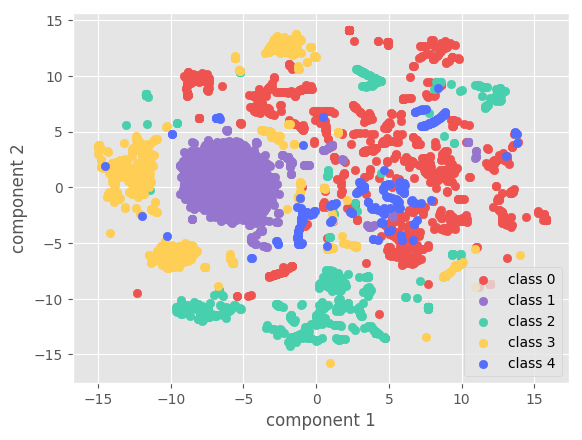 Figure 20
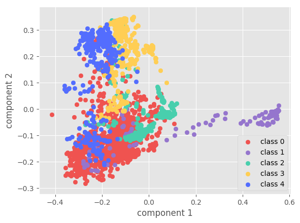 Figure 21
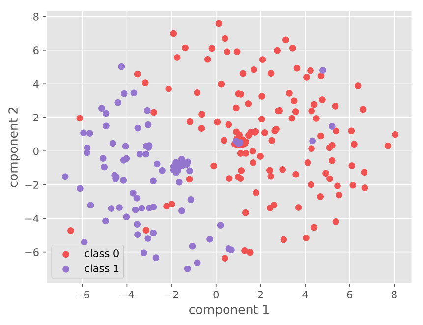 Figure 22
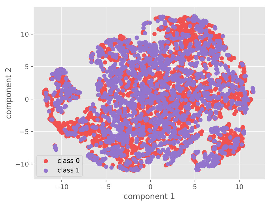 Figure 23
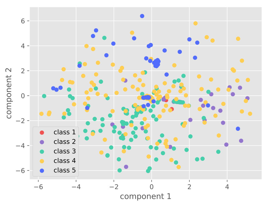 Figure 24
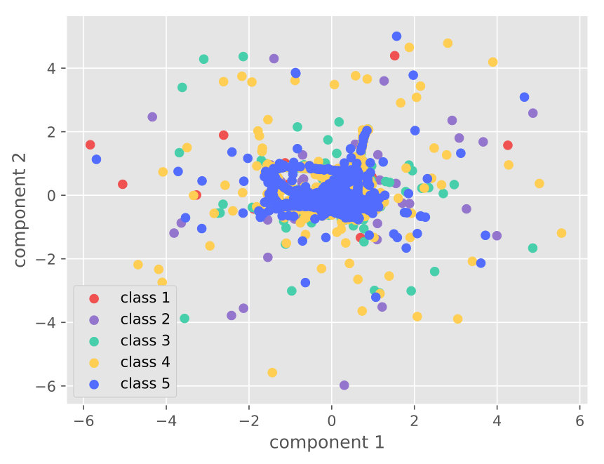 Figure 25
| Dataset | Rate (%) | Algorithm-related State-of-the-art | Application-related State-of-the-art | Ablation Study | Ours | ||||||||
|---|---|---|---|---|---|---|---|---|---|---|---|---|---|
| M2 | AAE | LVAE | ADGM | (Chen et al., 2018) | (Lara et al., 2012) | (Guo et al., 2016) | (Zhang et al., 2018) | VAE () | VAE | VAE++ | AVAE | ||
| Activity Recognition (PAMAP2) | 20 | 64.830.16 | 63.670.23 | 69.820.69 | 67.310.45 | 72.310.16 | 70.950.08 | 67.310.14 | 76.680.31 | 58.430.13 | 76.510.53 | 78.120.55 | 78.630.38 |
| 40 | 68.920.23 | 76.830.25 | 76.430.19 | 78.210.38 | 80.510.21 | 75.380.12 | 77.280.21 | 80.150.16 | 62.740.12 | 78.780.22 | 80.880.38 | 81.370.29 | |
| 60 | 72.350.21 | 77.390.19 | 78.690.27 | 79.340.29 | 80.290.21 | 76.890.05 | 79.690.15 | 82.490.33 | 67.850.08 | 79.630.29 | 81.940.19 | 84.910.17 | |
| 80 | 75.880.35 | 78.280.11 | 81.410.23 | 80.380.16 | 82.120.16 | 79.950.18 | 81.650.09 | 83.560.11 | 73.430.06 | 81.750.17 | 82.080.26 | 85.560.21 | |
| 100 | 77.590.17 | 80.790.14 | 84.390.18 | 83.660.16 | 83.640.12 | 81.960.11 | 82.380.13 | 84.590.24 | 76.850.00 | 82.370.25 | 83.290.18 | 86.410.06 | |
| Dataset | Rate (%) | Algorithm-related State-of-the-art | Application-related State-of-the-art | Ablation Study | Ours | ||||||||
|---|---|---|---|---|---|---|---|---|---|---|---|---|---|
| M2 | AAE | LVAE | ADGM | (Ziyabari et al., 2017) | (Harati et al., 2015) | (Schirrmeister et al., 2017) | (Goodwin and Harabagiu, 2017) | VAE () | VAE | VAE++ | AVAE | ||
| Neurological Diagnosis (TUH) | 20 | 71.280.16 | 80.130.95 | 82.310.19 | 86.320.12 | 87.660.23 | 86.380.36 | 82.190.24 | 86.330.21 | 80.580.69 | 86.370.24 | 0.860.53 | 93.690.16 |
| 40 | 75.320.16 | 82.950.26 | 84.380.16 | 86.990.05 | 89.250.19 | 91.580.35 | 84.210.08 | 89.250.34 | 81.350.24 | 89.690.27 | 91.280.25 | 94.320.28 | |
| 60 | 76.320.29 | 86.210.52 | 87.510.26 | 87.650.16 | 91.280.37 | 92.580.26 | 85.360.32 | 90.380.24 | 82.590.63 | 90.580.27 | 92.870.31 | 95.210.21 | |
| 80 | 79.650.37 | 88.530.28 | 89.560.25 | 88.050.12 | 92.590.26 | 93.250.31 | 85.160.24 | 91.590.16 | 83.210.21 | 91.690.35 | 93.960.28 | 97.860.26 | |
| 100 | 82.590.31 | 89.580.25 | 90.250.21 | 88.650.26 | 93.320.18 | 94.290.25 | 86.420.26 | 92.40.25 | 84.210.65 | 92.380.41 | 94.650.24 | 98.130.32 | |
| Dataset | Rate (%) | Algorithm-related State-of-the-art | Application-related State-of-the-art | Ablation Study | Ours | ||||||||
|---|---|---|---|---|---|---|---|---|---|---|---|---|---|
| M2 | AAE | LVAE | ADGM | (Odena, 2016) | (Springenberg, 2016) | (Weston et al., 2012) | (Miyato et al., 2018) | VAE () | VAE | VAE++ | AVAE | ||
| Image Classification (MNIST) | 20 | 93.220.62 | 90.250.25 | 93.250.26 | 89.610.27 | 95.230.34 | 94.250.13 | 94.580.25 | 92.960.28 | 91.580.24 | 92.310.53 | 93.590.31 | 95.120.19 |
| 40 | 93.250.34 | 93.210.23 | 93.280.46 | 91.580.25 | 95.270.53 | 95.560.08 | 95.210.26 | 93.210.56 | 93.650.21 | 94.210.19 | 94.680.28 | 96.430.35 | |
| 60 | 96.240.51 | 96.350.27 | 95.340.21 | 93.210.34 | 96.380.22 | 96.540.08 | 96.480.32 | 96.280.57 | 94.890.21 | 95.340.14 | 96.420.25 | 97.210.21 | |
| 80 | 98.190.25 | 95.320.37 | 96.110.52 | 95.010.15 | 97.820.11 | 97.210.13 | 97.860.34 | 97.630.15 | 96.780.25 | 97.630.15 | 98.710.16 | 99.790.12 | |
| 100 | 98.650.21 | 0.98.250.61 | 96.350.26 | 95.380.82 | 99.210.26 | 98.640.27 | 99.060.22 | 98.530.17 | 97.410.18 | 98.350.09 | 99.670.23 | 99.850.11 | |
| Dataset | Rate (%) | Algorithm-related State-of-the-art | Application-related State-of-the-art | Ablation Study | Ours | ||||||||
|---|---|---|---|---|---|---|---|---|---|---|---|---|---|
| M2 | AAE | LVAE | ADGM | (Pazzani and Billsus, 2007) | (Rendle, 2012) | (He and Chua, 2017) | (Chen et al., 2017) | VAE () | VAE | VAE++ | AVAE | ||
| Recommender System (Yelp) | 66.420.17 | 58.270.35 | 66.350.36 | 54.270.38 | 40.550.27 | 47.580.36 | 65.990.62 | 66.210.24 | 64.280.12 | 64.390.62 | 65.580.37 | 70.190.87 | |
| 20 | 69.360.37 | 61.550.62 | 68.160.24 | 55.350.26 | 40.280.32 | 48.650.27 | 67.530.31 | 66.590.29 | 64.370.25 | 67.230.95 | 71.050.29 | 72.210.35 | |
| 40 | 72.580.19 | 62.150.39 | 68.590.93 | 57.630.23 | 42.150.16 | 50.950.24 | 66.580.29 | 67.950.38 | 67.560.35 | 69.580.37 | 72.190.62 | 75.340.35 | |
| 60 | 72.390.64 | 62.890.62 | 74.280.37 | 58.340.15 | 43.210.15 | 52.150.38 | 67.650.31 | 68.230.15 | 69.250.18 | 71.390.56 | 73.210.58 | 78.540.38 | |
| 80 | 74.580.62 | 63.510.86 | 72.590.36 | 59.580.23 | 45.860.22 | 54.100.12 | 68.030.17 | 70.610.25 | 73.240.68 | 73.280.69 | 76.530.28 | 79.380.59 | |
Peer Reviews
No public reviews on file for this paper yet. If you reviewed it on a platform where reviews are public (OpenReview, ICLR, NeurIPS, ICML), you can paste yours below so the community can read it here.
Code & Models
Videos
No videos yet. Explain this paper in a talk, walkthrough, or lecture? Add one.
Taxonomy
MethodsSolana Customer Service Number +1-833-534-1729 · Convolution · USD Coin Customer Service Number +1-833-534-1729 · Dogecoin Customer Service Number +1-833-534-1729
Adversarial Variational Embedding for Robust Semi-supervised Learning
Xiang Zhang, Lina Yao, Feng Yuan
University of New South Wales, Sydney, Australia
[email protected], [email protected], [email protected]
(2019)
Abstract.
Semi-supervised learning is sought for leveraging the unlabelled data when labelled data is difficult or expensive to acquire. Deep generative models (e.g., Variational Autoencoder (VAE)) and semi-supervised Generative Adversarial Networks (GANs) have recently shown promising performance in semi-supervised classification for the excellent discriminative representing ability. However, the latent code learned by the traditional VAE is not exclusive (repeatable) for a specific input sample, which prevents it from excellent classification performance. In particular, the learned latent representation depends on a non-exclusive component which is stochastically sampled from the prior distribution. Moreover, the semi-supervised GAN models generate data from pre-defined distribution (e.g., Gaussian noises) which is independent of the input data distribution and may obstruct the convergence and is difficult to control the distribution of the generated data. To address the aforementioned issues, we propose a novel Adversarial Variational Embedding (AVAE) framework for robust and effective semi-supervised learning to leverage both the advantage of GAN as a high quality generative model and VAE as a posterior distribution learner. The proposed approach first produces an exclusive latent code by the model which we call VAE++, and meanwhile, provides a meaningful prior distribution for the generator of GAN. The proposed approach is evaluated over four different real-world applications and we show that our method outperforms the state-of-the-art models, which confirms that the combination of VAE++ and GAN can provide significant improvements in semi-supervised classification.
Variational Autoencoder, Generative Adversarial Networks, Representation Learning, Semi-supervised Classification
††journalyear: 2019††copyright: acmcopyright††conference: The 25th ACM SIGKDD Conference on Knowledge Discovery and Data Mining; August 4–8, 2019; Anchorage, AK, USA††booktitle: The 25th ACM SIGKDD Conference on Knowledge Discovery and Data Mining (KDD ’19), August 4–8, 2019, Anchorage, AK, USA††price: 15.00††doi: 10.1145/3292500.3330966††isbn: 978-1-4503-6201-6/19/08
1. Introduction
Semi-supervised learning from data is one of the fundamental challenges in artificial intelligence, which considers the problem when only a subset of the observations has corresponding class labels (Ghasedi Dizaji et al., 2018). This issue is of immense practical interest in a broad range of application scenarios, such as abnormal activity detection (Yao et al., 2016), neurological diagnosis (Peng et al., 2016), computer vision (Gong et al., 2016), and recommender systems (Yang et al., 2017). In these scenarios, it is easy to obtain abundant observations but expensive to gather the corresponding class labels. Among existing approaches, Variational Autoencoders (VAEs) (Kingma et al., 2014; Sønderby et al., 2016) have recently achieved state-of-the-art performance in semi-supervised learning.
VAE models provide a general framework for learning latent representations: a model is specified by a joint probability distribution both over the data and over latent random variables, and a representation can be found by considering the posterior on latent variables given specific data (Narayanaswamy et al., 2017). The learned representations can not only be used for generation but also for classification. For instance, VAE provides a latent feature representation of the input observations, where a separate classifier can be thereafter trained using these representations. The high quality of latent representations enables accurate classification, even with a limited number of labels. A number of studies have applied VAE in semi-supervised classification in the computer vision area (Kingma et al., 2014; Makhzani et al., 2015; Narayanaswamy et al., 2017).
1.1. Motivation
Why we propose the VAE++ . One major challenge faced by the existing VAE-based semi-supervised methods is that the latent representations are stochastically sampled from the prior distribution instead of being directly rendered from the explicit observations. In particular, as shown in Figure 1(a), the learned latent representations are randomly sampled from a multivariate Gaussian distribution (see Equation 1). Thus, for a specific sample, the corresponding latent representation is not exclusive (i.e., the representation is not repeatable in different runnings), which makes it inappropriate for classification. To solve this problem, in the latent space, we propose a new variable (see Figure 1(b)) which is directly learned from the input data. The exclusive latent code is guaranteed to keep invariant for a specific input in different runnings. The modified VAE is called VAE++. In addition, the learned expectation only contains a part of information of the input observations, which is not enough to represent the observations in classification task, even though is exclusive111For the same reason, can not be used as the exclusive code.. The comparison of performance among , and will be presented in Section 4.
Why VAE++ needs the semi-supervised GAN. In the proposed VAE++, it is necessary to reduce the information loss between the two latent representations and to guarantee the learned is representative. The commonly used constraints between two distributions (e.g., Kullback-Leibler divergence) can only utilize the information of the observations but fail to exploit the information of labels. In this paper, we use a novel approach to take advantage of both unlabelled and labelled data by jointly training the VAE++ and a semi-supervised GAN.
Why semi-supervised GAN needs the VAE++. GAN based approaches (Odena, 2016; Salimans et al., 2016) have recently shown promising results in semi-supervised learning. The semi-supervised GAN trains a generative model and a discriminator with inputs belonging to one of classes. Different from the regular GAN, the semi-supervised GAN requires the discriminator to make a class prediction with an extra class added, corresponding to the generated fake samples. In this way, the observations’ properties can be used to improve decision boundaries and allow for more accurate classification than using the labelled data alone. However, the generated samples are sampled from pre-defined distribution (e.g., Gaussian noise) (Cao et al., 2018). Such pre-defined prior distributions are often independent from the input data distributions and may obstruct the convergence and can not guarantee the distribution of the generated data. This drawback can be amended by gearing with VAE++ which can provide a meaningful prior distribution that can represent the distribution of the input data.
We introduce a recipe for semi-supervised learning, a robust Adversarial Variational Embedding (AVAE) framework, which learns the exclusive latent representations by combining VAE and semi-supervised GAN. To utilize the generative ability of GAN and the distribution approximating power of VAE, the proposed approach employs GAN to encourage VAE for the aim of learning the more robust and informative latent code. We present the framework in the context of VAE, adding a new exclusive code in latent space which is directly rendered from the data space. The generator in VAE++ also works as a generator of GAN. Both the exclusive code (marked as real) and the generated representation (marked as fake) are fed into the discriminator in order to force them to have similar distribution (Mirza and Osindero, 2014).
1.2. Contribution
Although a small set of models combining VAE and GAN have been previously explored, they are all focused on the generation perspective. To our knowledge, we are in the first batch of work that focuses on classification by aggregating VAE and GAN. We mark the following contributions:
- •
We present a novel semi-supervised Adversarial Variational Embedding approach to harness the deep generative model and generative adversarial networks collectively under a trainable unified framework. The reproducible codes and datasets are publicly available222https://github.com/xiangzhang1015/Adversarial-Variational-Semi-supervised-Learning.
- •
We propose a new structure, VAE++, to automatically learn an exclusive latent code for accurate classification. A novel semi-supervised GAN, which exploits both the unlabelled data distribution and categorical information, is proposed to gear with the VAE++ in order to encourage the VAE++ to learn a more effective and robust exclusive code.
- •
We evaluate the proposed approach over four real-world applications (activity reconstruction, neurological diagnosis, image classification, and recommender system). The results demonstrate that our approach outperforms all the state-of-the-art methods.
2. Related Work
There are a host of studies that have been investigated to apply VAE for semi-supervised learning (Kingma et al., 2014; Narayanaswamy et al., 2017; Sønderby et al., 2016; Maaløe et al., 2016). (Kingma et al., 2014) explores semi-supervised learning with deep generative models by building two VAE-based deep generative models for latent representation extraction. Afterward, (Narayanaswamy et al., 2017) attempts to learn disentangled representations that encode distinct aspects of the data into separate variables. However, in all the existing semi-supervised VAE models, the learned representations do not only depend on the posterior distribution but also on the latent random variables. It is necessary that learning the exclusive code which is only related to the posterior distribution for the specified data.
Another recent arising semi-supervised method is semi-supervised GAN (Odena, 2016; Springenberg, 2016; Radford et al., 2016). SGAN (Odena, 2016) extends GAN to the semi-supervised context by forcing the discriminator network to output class labels. The CatGAN (Springenberg, 2016) modifies the objective function to take into account the mutual information between observed examples and their predicted class distributions. In the above methods, the generator chooses simple factored continuous noise which is independent from the input data distribution, for generation. As a result, it is possible that the noise will be used by the generator in a highly entangled way, increasing the difficulty to control the distribution of the generated data. Conditional GAN (Mirza and Osindero, 2014) and InfoGAN (Chen et al., 2016) address this drawback by utilizing external information (e.g., categorical information) as a restriction, but they both pay attention to generation or supervised classification and have limited help in semi-supervised classification.
Despite the few works attempting to combine VAE and GAN (Larsen et al., 2015; Makhzani et al., 2015; Bao et al., 2017), most of them focus on generation instead of classification. For example, the VAE/GAN (Larsen et al., 2015) and CVAE-GAN (Bao et al., 2017) employ the standard VAE to share the encoder with the generator of GAN in order to generate new observations. For semi-supervised classification, we care about the latent code instead of the observations. The Adversarial Autoencoder (AAE (Makhzani et al., 2015)) integrates VAE and GAN but only employs GAN to replace KL divergence as a penalty to impose a prior distribution on the latent code, which is a totally different direction from our work.
Summary. Unlike the existing VAE- and GAN-based studies, the proposed model 1) focuses on semi-supervised classification instead of generation; 2) attempts to learn an exclusive latent representation instead of a stochastic sampled representation; 3) works on improvement of latent space instead of data space. Moreover, the semi-supervised GAN in our work partly adopts the improved GAN (Salimans et al., 2016), but there are a number of differences: 1) (Salimans et al., 2016) adopts the semi-supervised strategy for classification while we adopt this strategy as a constraint to reduce information loss in the transformation from to in order to force the proposed AVAE to learn a more robust and effective latent code; 2) (Salimans et al., 2016) employs the discriminator of GAN as the classifier while we adopt an extra non-parametric classifier since the former has poor performance in our case (take the PAMAP2 dataset as an example, (Salimans et al., 2016) and our model achieve the accuracy around 65% and 85%, respectively); 3) we employ weighted loss function to balance the significance of the unlabelled and labelled observations.
3. Methodology
Suppose the input dataset has two subsets, one of which contains labelled samples while the other contains unlabelled samples. In the former subset, the observations appear as pairs with the -th observation and the corresponding one-hot label where denotes the number of classes. denotes the number of labelled observations while denotes the number of the observation dimensions. In the latter subset, only the observations are available and denotes the number of unlabelled observations . The total data size equals to the sum of and . In terms of effective classification, we attempt to learn a latent representation which is rich of distinguishable information. Then the learned representations can be fed into a classifier for recognition. In this paper, we mainly focus on the latent code learning.
In the semi-supervised learning, due to the lack of labelled observations, it is significant to learn latent variable distribution based on the observations without label333For simplification, we omit the index and directly use variable to denote observations.. Thus, we are required to build an encoder to provide an embedding or feature representation which allows accurate classification even with limited observations.
3.1. VAE++
The VAE is demonstrated to provide a latent feature representation for semi-supervised learning (Kingma et al., 2014; Narayanaswamy et al., 2017), compared to a linear embedding method or a regular autoencoder. The VAE maps the input observation to a compressed code , and decodes it to reconstruct the observation. The latent representation is calculated through the reparameterization trick (Kingma and Welling, 2013):
[TABLE]
with to impose the posterior distribution of the latent code on . and denote the expectation and standard deviation of the posterior distribution of , which are learned from . For the efficient generation and reconstruction, VAE imposes the code on a prior Gaussian distribution:
[TABLE]
Through minimizing the reconstruction error between and and restricting the distribution of to approximate the prior distribution , VAE is supposed to learn the representative latent code which can be used for classification or generation.
Due to the strong feature representation ability, VAE has been employed for feature extraction and semi-supervised learning (Abbasnejad et al., 2017; Xu et al., 2017; Walker et al., 2016; Narayanaswamy et al., 2017). However, one limitation of the standard VAE is that the learned latent code , as shown in Equation (1), is not exclusive. In other words, for a specific observation and a fixed embedding model , the corresponding latent code is not exclusive as it contains a stochastic variable which is randomly sampled from the prior distribution . For instance, in a pre-trained fixed VAE encoder, the specific input will lead to a variety of in different running. At high level, the latent code is determined by two factors: the prior distribution of observation which affects through the learned and , and the stochastically sampled data . However, the stochastically sampled latent code is unstable and will corrupt the features for classification. Furthermore, the posterior distribution of is forced to approximate the manually set prior distribution (commonly Normal Gaussian distribution), which inevitably leads to information loss.
In order to completely sidestep the above-mentioned issue, in this paper, we propose a novel VAE++ model to learn an exclusive latent code . The VAE++ contains three key components: the encoder, the generator, and the decoder (see Figure 2). The encoder transforms the observation into a latent code which is directly determined by the input . denotes the dimension of . We learn the:
[TABLE]
where denotes a non-linear transformation while denotes encoder parameters. The non-linear transformation is generally chosen as a deep neural network for the excellent ability of non-linear approximation. Then, in the generator, we measure the expectation and the standard derivation from the latent code and update Equation (1). The generated variable can be calculated by:
[TABLE]
At last, the decoder is employed to reconstruct the sample:
[TABLE]
where denotes another non-linear rendering, called decoder, with parameters and denotes the reconstructed observation.
The loss function of VAE++ can be calculated by:
[TABLE]
The first component is the reconstruction loss, which equals to the expected negative log-likelihood of the observation. This term encourages the decoder to reconstruct the observation based on the sampling code which is under Gaussian distribution. The lower reconstruction error indicates the encoder learned a better latent representation. The second component is the Kullback-Leibler divergence which measures the distance between the prior distribution of the latent code and the posterior distribution . This divergence reflects the information loss when we use to represent .
In the latent space of the novel VAE++, there are two compressed informative codes and . The former represents directly-encoded whilst the latter is stochastically sampled from the posterior distribution , which makes the former more suitable for classification. Therefore, we choose as the compressed latent code in VAE++ instead of the in standard VAE.
From equation (2), we can observe that the expectation and standard deviation of and are invariant. In particular, for a specific sample , the corresponding and have the same statistical characteristics. Thus, we have
[TABLE]
which indicates that the generated is affected by both the distribution (or statistic characteristics) of and the prior distribution (or ). In summary, the inherits the statistical characteristics of .
3.2. Adversarial Variational Embedding
One significant sufficient condition of a well-trained VAE++ is less information loss in the transformation from to to guarantee the learned is representative. As mentioned before, the information in is partly inherited from and the other part is randomly sampled from the prior distribution . Since the conditional distribution has a better description of the input observation , we attempt to increase the proportion of inherited part and decrease the proportion of stochastically sampled part.
As shown in Figure 2, in the proposed AVAE the generator generates based on the joint probability instead of the noise in standard GAN. The is regarded as ‘fake’ while is marked as ‘real’. Specifically, for the labelled observations , VAE++ encodes the input to the latent code and generates ; similarly, for unlabelled observations , we have and generates . To exploit the information of the labels, we extend the which has possible classes to which has possible classes by regarding the generated fake samples as the -th class (Salimans et al., 2016; Odena, 2016). In the VAE++, the unspecified denotes both and whenever we don’t care whether the observation is labelled or not. This rule also applies to . Similarly, we use to denote the input of the discriminator , which contains both and . The discriminator can be described by
[TABLE]
where denotes the parameters of while denotes the non-linear transformation which is implemented by a Convolutional Neural Networks (CNN) (Krizhevsky et al., 2012) in this paper. Therefore, we can use to supply the probability where is fake (from ) and use to supply the probability where is real ((from )) and is correctly classified.
For the labelled input, same as supervised learning, the discriminator is supposed to not only tell whether the input is real or generated, but also classify it into the correct class. Therefore, we have the supervised loss function
[TABLE]
where denotes the joint probability.
For the unlabelled input, we only require the discriminator to perform a binary classification: the input is real or fake. The former probability can be calculated by whilst the latter can be calculated by . Thus, the unsupervised loss function:
[TABLE]
In summary, the final loss function of the discriminator
[TABLE]
where are weights and is a switch function
[TABLE]
If the specific observation is labelled, we calculate the labelled loss function. Otherwise, we calculate the unlabelled loss function. From empirical experiments, we observe that the is much easier to converge than and the real/fake classification accuracy is much higher than the classes classification accuracy. To encourage the optimizer to focus on the former part which is more difficult to converge, we set and .
The discriminator receives as input and extracts the dependencies through CNN filters. Two fully connected layers follow the convolutional layer for dimension reduction. At last, a softmax layer is employed to work on the low-dimension features to estimate the log normalization of the categorical probability distribution which is output as .
The overall aim of the proposed AVAE (as described in Algorithm 1) is to train a robust and effective semi-supervised embedding method. The VAE loss and the GAN loss are trained simultaneously by the Adam optimizer. After convergence, the compressed representative code is fed into a non-parametric nearest neighbors classifier for recognition.
4. Experiments
In this section, we demonstrate the effectiveness and validation of the proposed method over four applications.
4.1. Activity Recognition
4.1.1. Experiment Setup
Activity recognition is an important area in data mining. We evaluate our approach over the well-known PAMAP2 dataset (Fida et al., 2015), which is collected by 9 participants (8 males and 1 female) aged . We select 5 most commonly used activities (Cycling, standing, walking, lying, and running, labelled from 0 to 4) as a subset for evaluation. For each subject, there are 12,000 instances. The activity is measured by 3 Inertial Measurement Units (IMU) attached to the participants’ wrist, chest, and the outer ankle. Each IMU includes 13 dimensions: two 3-axis accelerometers, one 3-axis gyroscopes, one 3-axis magnetometers and one thermometer. The experiments are performed by a Leave-One-Subject-Out strategy to ensure the practicality.
The time window is set as 10 with 50% overlapping. The dataset is split into a training set (80% proportion) and a testing set (20% proportion). For semi-supervised learning, the training dataset contains both labelled observations and unlabelled observations. We present a term called‘supervision rate’ as a handle on the relative weight between the supervised and unsupervised terms. For the given number of labelled observations and the number of unlabelled observations , the supervision rate is defined by .
4.1.2. Parameter Setting
We introduce the default parameter settings and the settings in other applications keep the same if not mentioned. The input observations are first normalized by Z-score normalization and fed to the input layer of the unsupervised VAE++. The neuron amount in the first hidden layer, which is denoted by , is a quarter of . The second hidden layer contains 2 components which represent the expectation and the standard deviation respectively. The third hidden layer has the sample shape with . An Adam optimizer with a learning rate of is employed to minimize the loss function of VAE++.
After each epoch of VAE++, the first hidden layer and the third hidden layer are labelled as ‘real’ and ‘fake’, respectively, and fed to the discriminator . The discriminator contains one convolutional layer followed by two fully-connected layers. There is a softmax layer to obtain the categorical probability before the output layer which has neurons. The convolutional layer has 10 filters which have shape and the stride size . The padding method of the convolutional operation is set as ‘same’ while the activation function is ReLU. The following hidden layer has neurons and the sigmoid activation function. The loss function is optimized by Adam update rule with learning rate of . The object functions of the VAE++ and the discriminator are trained simultaneously. After the convergence of the proposed method, the semi-supervised learned latent representation is fed into a supervised non-parametric nearest neighbor classifiers with .
4.1.3. Baselines
To measure the effectiveness of the proposed method, we compare it with a set of competitive state-of-the-art models. The state-of-the-art methods are composed of two categories: algorithm-related and application-related. The former denotes other VAE/GAN based semi-supervised classification algorithms, which are the same for all the applications. The comparison is used to demonstrate our framework has the highest semi-supervised representation learning ability. The latter denotes the state-of-the-art models in each application, which are varied for the different applications. The comparison is used to demonstrate our work is effective in the real-world scenarios.
The algorithm-related semi-supervised learning solutions in our comparison are listed as follows:
- •
M2. (Kingma et al., 2014) proposes a probabilistic model that describes the data as being generated by a latent class variable in addition to a continuous latent representation.
- •
Adversarial Autoencoders (AAE). (Makhzani et al., 2015) employs the GAN to perform variational inference by matching the aggregated posterior of the hidden representation of the autoencoder.
- •
Ladder Variational Autoencoders (LVAE). (Sønderby et al., 2016) proposes an inference model which recursively corrects the generative distribution by a data dependent likelihood.
- •
Auxiliary Deep Generative Models (ADGM). (Maaløe et al., 2016) extends deep generative models with auxiliary variables, which improves the variational approximation.
We design ablation study to demonstrate the necessity of each key component of the proposed approach. In the ablation study, we set four control experiments with single variable among the components of AVAE. We adopt the following four methods to discover the latent representations: 1) VAE () with as the latent representation; 2) standard VAE ( as the latent representation); 3) VAE++ ( as the latent representation); 4) AVAE. The extracted representations are fed into the same classifier for final classification.
The application-related state-of-the-art models on activity recognition are listed here:
- •
Chen et al. (Chen et al., 2018) adopt an attention mechanism to select the most distinguishable features from the activity signals and send them to a CNN structure for classification.
- •
Lara et al. (Lara et al., 2012) apply both statistical and structural detectors features to discriminate among activities.
- •
Guo et al. (Guo et al., 2016) exploit the diversity of base classifiers to construct a good ensemble for multimodal activity recognition, and the diversity measure is obtained from both labelled and unlabelled data.
- •
Zhang et al. (Zhang et al., 2018) combine deep learning and the reinforcement learning scheme to focus on the crucial dimensions of the signals.
4.1.4. Results and Discussion
First, we report the overall performance of all the compared algorithms. From Table 1, we can observe that the proposed approach (AVAE) outperforms all the algorithm-related and application-related state-of-the-art models, illustrating the effectiveness of the latent space in providing robust representations for easier semi-supervised classification. The advantage is demonstrated under all the supervision rates.
In Table 1, through the ablation study, it is observed that each component (especially GAN) contributes to the performance enhancement. Additionally, the proposed AVAE achieves a significant improvement which yields around and growth than the standard VAE and the VAE++ (under 60% supervision rate), respectively. This observation demonstrates that the proposed latent layer and the adversarial training (between the discriminator and VAE++) encourages the proposed model to learn and refine the informative latent code. Take 60% supervision rate as an example, more details of the classification are shown in the confusion matrix (Figure 3(a)) and ROC curves with AUC score (Figure 4(a)).
4.2. Neurological Diagnosis
4.2.1. Experiment Setup
EEG signal collected in the unhealthy state differs significantly from the ones collected in the normal state (Adeli et al., 2007). The epileptic seizure is a common brain disorder that affects about 1% of the population and its octal state could be detected by the EEG analysis of the patient. In this application, we evaluate our framework with raw EEG data to diagnose the epileptic seizure of the patient.
We choose the benchmark dataset TUH (Obeid and Picone, 2016) for epileptic seizure diagnosis. The TUH is a neurological seizure dataset of clinical EEG recordings associated with 22 channels from a 10/20 configuration. The sampling rate is set as 250 Hz. We select 12,000 samples from each of 18 subjects. Half of the samples are labelled as epileptic seizure state (labelled as 1) and the remaining samples are labelled as normal state (labelled as 0). The experiment and parameter settings are the same as the activity recognition applications.
4.2.2. Baselines
The application-related state-of-the-art approaches in neurological diagnosis are listed here:
- •
Ziyabari et al. (Ziyabari et al., 2017) adopt a hybrid deep learning architecture, including LSTM and stacked denoising Autoencoder, which integrates temporal and spatial context to detect the epileptic seizure.
- •
Harati et al. (Harati et al., 2015) demonstrate that a variant of the filter bank-based approach, coupled with first and second derivatives, provides a reduction in the overall error rate.
- •
Schimeister et al. (Schirrmeister et al., 2017) attempt to improve the performance of seizure detection by combining deep ConvNets with training strategies such as exponential linear units.
- •
Goodwin et al. (Goodwin and Harabagiu, 2017) combine RNN with access to textual data in EEG reports in order to automatically extracting word- and report-level features and infer underspecified information from EHRs (electronic health records).
4.2.3. Results and Discussion
From Table 2, we can observe that our approach outperforms all the competitive baselines on TUH dataset. For instance, under 60% supervision level, the proposed approach achieves the highest accuracy of 95.21% which claims around 4% improvement over other methods. The corresponding confusion matrix (Figure 3(b)) and ROC curves (Figure 4(b)) infer that the normal state has higher accuracy than the seizure state. One possible reason is that the start and end stage of the seizure has similar symptoms with the normal state which may lead to misclassification.
4.3. Image Classification
4.3.1. Experiment Setup
To evaluate the representation learning ability in images, we test our approach on the benchmark dataset MNIST 444http://yann.lecun.com/exdb/mnist/. MNIST contains 60,000 handwritten digital images (50,000 for training and 10,000 for testing) with pixels. The labels of this dataset are from 0 to 9, corresponding to the 10 digits.
4.3.2. Parameter Settings
Images are more informative compared to other application scenarios. The encoder of AVAE is designed to be stacked by two convolutional layers. The first convolutional layer has 32 filters with shape , the stride size , ’SAME’ padding, and ReLU activation function. The followed pooling layer has window size, stride, and ’SAME’ padding. The second convolutional layer has 64 filters with . The residual parameters of the second convolutional layer and the second pooling layer are the same with the former. Similarly, the decoder contains two de-convolutional layers with the same parameter settings.
4.3.3. Baselines
We reproduce the following methods under different supervision rate for comparison:
- •
Augustus (Odena, 2016) proposes a semi-supervised GAN (SGAN) by forcing the discriminator network to output class labels.
- •
Springenberg (Springenberg, 2016) proposes CatGAN to modify the objective function taking into account the mutual information between observation and the prediction distribution.
- •
Weston et al. (Weston et al., 2012) apply kernel methods for a nonlinear semi-supervised embedding algorithm.
- •
Miyato et al. (Miyato et al., 2018) propose a regularization method based on virtual adversarial loss: a new measure of local smoothness of the conditional label distribution given the inputs.
4.3.4. Results and Discussion
As shown in Table 3, AVAE outperforms the counterparts with a slight gain with the same supervision level. The confusion matrix and ROC curves are reported in Figure 3(c) and Figure 4(c). The results show that our approach is enabled to automatically learn the discriminative features by joint training the VAE++ and the semi-supervised GAN.
4.4. Recommender System
4.4.1. Experiment Setup
We apply our framework on recommender system scenarios, in particular, a restaurant rating prediction task based on the widely used Yelp dataset.
The Yelp Dataset555https://www.yelp.com/dataset which includes 192,609 Businesses, 1,637,138 Users, and 6,685,900 Ratings. Each business has 13 attributes (like ‘near garage?’, ‘have valet?’) which can describe the quality and convenience of the business. Meanwhile, each business is rated by a series customers. The ratings range from 1 to 5, which can reflect the customers’ satisfactory degree. Our recommender task considers a unseen business’s attributes as input data and predict the possible ratings from the potential customers. If the rating is high enough, the new business will be recommended to the public.
4.4.2. Baselines
We compare our approach with the state-of-the-art recommender system models which exploit the content information of items. Since these methods are used to make rating predictions for each user-item pair, we select those users who have 200 and more ratings in the Yelp dataset, generating a set of 1,111 users. After collecting the predicted ratings for all user-item pairs, we take the average item ratings over the users, which are further rounded to serve as the predicted labels.
- •
Pazzani et al. (Pazzani and Billsus, 2007) summarizes basic content-based recommendation approaches, from which we select the cosine similarity-based nearest neighbour method as our fundamental baseline.
- •
Rendle (Rendle, 2012) proposes the original implementation of factorization machine(FM) which is capable of incorporating item features with explicit feedbacks. We concatenate only the item indication vector and its feature after each user indication vector following the format in (Rendle, 2012).
- •
He et al. (He and Chua, 2017) enhances the original FM using deep neural networks to learn high-order interactions between different item features.
- •
Chen et al. (Chen et al., 2017) applies feature- and item-level attention on item features, which is capable of emphasizing on the most important features.
4.4.3. Results and Discussion
From Table 4, we can observe that our approach outperforms both the competitive semi-supervised algorithms and the content-based recommender system state-of-the-art methods. The rating prediction details can be found in Figure 3(d) and Figure 4(d). The classification performance in recommender system is not good as in other applications. One possible reason is that the attributes data are very sparse. The experiment results illustrate that our approach is effective in recommender system scenarios.
4.5. Further Analysis
4.5.1. Supervision Rate
We conduct extensive experiments to investigate the impact of supervision rate . The supervision rate ranges from 20% to 100% with 20% interval and each setting runs for at least three times with the average accuracy recorded. The overall performance varies with the supervision rate . From Table 2 to Table 4, it is noticed that the proposed model obtains competitive performance at each supervision level.
4.5.2. Visualization
Figure 5 visualizes the raw data and the learned features on different datasets. The visualization comparison demonstrates the capability of our approach for distinguishable feature learning.
4.5.3. Convergence
Take PAMAP2 as an example, Figure 6 presents the relationship between the loss function values and the epoch numbers. The VAE++ loss includes the reconstruction loss and the KL-divergence whilst the loss of the discriminator in GAN includes labelled loss and unlabelled loss (with weights 0.9 and 0.1, respectively). We can observe that the proposed method shows good convergence property as it stablizes in around 200 epochs.
5. Conclusion
In this paper, we present an effective and robust semi-supervised latent representation framework, AVAE, by proposing a modified VAE model and integration with generative adversarial networks. The VAE++ and GAN share the same generator. In order to automatically learn the exclusive latent code, in the VAE++, we explore the latent code’s posterior distribution and then stochastically generate a latent representation based on the posterior distribution. The discrepancy between the learned exclusive latent code and the generated latent representation is constrained by semi-supervised GAN. The latent code of AVAE is finally served as the learned feature for classification. The proposed approach is evaluated on four real-world applications and the results demonstrate the effectiveness and robustness of our model.
The hyper-parameter tuning (not presented in this paper due to space limitation) in our model is required for different datasets in various applications. One of our future scope is to propose a more generalized framework which is not sensitive to datasets. Moreover, our model still requires adequate labelled training samples for good performance. The lower supervision rate or unsupervised learning is another major goal in the future.
6. Acknowledgement
This research was partially supported by grant ONRG NICOP N62909-19-1-2009.
The reference list from the paper itself. Each links out to its DOI / PubMed record.
- 1(1)
- 2Abbasnejad et al . (2017) M Ehsan Abbasnejad, Anthony Dick, and Anton van den Hengel. 2017. Infinite variational autoencoder for semi-supervised learning. In 2017 IEEE Conference on Computer Vision and Pattern Recognition (CVPR) . IEEE, 781–790.
- 3Adeli et al . (2007) Hojjat Adeli, Samanwoy Ghosh-Dastidar, and Nahid Dadmehr. 2007. A wavelet-chaos methodology for analysis of EE Gs and EEG subbands to detect seizure and epilepsy. IEEE Transactions on Biomedical Engineering 54, 2 (2007), 205–211.
- 4Bao et al . (2017) Jianmin Bao, Dong Chen, Fang Wen, Houqiang Li, and Gang Hua. 2017. CVAE-GAN: fine-grained image generation through asymmetric training. Co RR, abs/1703.10155 5 (2017).
- 5Cao et al . (2018) Jiezhang Cao, Yong Guo, Qingyao Wu, Chunhua Shen, and Mingkui Tan. 2018. Adversarial Learning with Local Coordinate Coding. The International Conference of Machine Learning (ICML) (2018).
- 6Chen et al . (2017) Jingyuan Chen, Hanwang Zhang, Xiangnan He, Liqiang Nie, Wei Liu, and Tat-Seng Chua. 2017. Attentive collaborative filtering: Multimedia recommendation with item-and component-level attention. In SIGIR . ACM, 335–344.
- 7Chen et al . (2018) Kaixuan Chen, Lina Yao, Xianzhi Wang, Dalin Zhang, Tao Gu, Zhiwen Yu, and Zheng Yang. 2018. Interpretable Parallel Recurrent Neural Networks with Convolutional Attentions for Multi-Modality Activity Modeling. International Joint Conference on Neural Networks (IJCNN) (2018).
- 8Chen et al . (2016) Xi Chen, Yan Duan, Rein Houthooft, John Schulman, Ilya Sutskever, and Pieter Abbeel. 2016. Infogan: Interpretable representation learning by information maximizing generative adversarial nets. In Advances in neural information processing systems . 2172–2180.
