
TL;DR
This paper analyzes the spectral properties of the harmonic mean of Wishart matrices using free probability, revealing how it compares to the arithmetic mean in operator norm for different sample sizes.
Contribution
It introduces a free probability approach to characterize the harmonic mean of Wishart matrices and uncovers a size-dependent norm closeness phenomenon.
Findings
Harmonic mean is closer to expectation than arithmetic mean for small n.
Operator norm difference varies with the number of matrices.
Results extend to non-identity expectation cases.
Abstract
We use free probability to compute the limiting spectral properties of the harmonic mean of i.i.d. Wishart random matrices whose limiting aspect ratio is when . We demonstrate an interesting phenomenon where the harmonic mean of the Wishart matrices is closer in operator norm to than the arithmetic mean for small , after which the arithmetic mean is closer. We also prove some results for the general case where the expectation of the Wishart matrices are not the identity matrix.
Click any figure to enlarge with its caption.
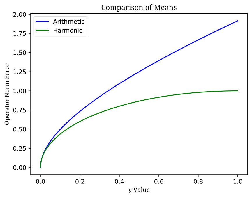 Figure 1
 Figure 2
Peer Reviews
No public reviews on file for this paper yet. If you reviewed it on a platform where reviews are public (OpenReview, ICLR, NeurIPS, ICML), you can paste yours below so the community can read it here.
Videos
No videos yet. Explain this paper in a talk, walkthrough, or lecture? Add one.
Harmonic Means of Wishart Random Matrices
Asad Lodhia
256 West Hall, 1085 South University Avenue, Ann Arbor MI, 48109-1107
Abstract.
We use free probability to compute the limiting spectral properties of the harmonic mean of i.i.d. Wishart random matrices whose limiting aspect ratio is when . We demonstrate an interesting phenomenon where the harmonic mean of the Wishart matrices is closer in operator norm to than the arithmetic mean for small , after which the arithmetic mean is closer. We also prove some results for the general case where the expectation of the Wishart matrices are not the identity matrix.
1. Introduction
Positive definite random matrices are often studied in probability theory and statistics. The most famous (and arguably most widely used) matrix model supported on the set of positive semidefinite matrices is the Wishart ensemble. Let be a sequence of centered independent identically distributed matrices that have dimension whose entries have at least two finite moments. Suppose each column of is an independent -dimensional random vector. The matrices
[TABLE]
are called Wishart matrices. If the columns of each are i.i.d. observations from a Gaussian distribution it suffices to specify their covariance matrix to obtain their distribution. In statistics the estimation of such a covariance matrix is a fundamental task. Our interest in this paper will be the mathematical study of estimates in operator norm of the covariance in the high-dimensional regime .
The notational choice in the previous paragraph may seem odd to the reader. If the columns of are drawn i.i.d., one may combine them, say by computing the arithmetic mean
[TABLE]
This reduces the variance by a factor of and is equivalent to adjoining the columns of the into a single -by- matrix, since
[TABLE]
In the regime where the sample covariance matrix does not converge to its expected value . Instead, when , the spectral measure of each satisfies the Marčenko-Pastur Law with parameter :
[TABLE]
In fact, under sufficient moment conditions [16], we have the stronger result that
[TABLE]
where represents the operator norm of the matrix . It is important to note here that the value of the operator norm in this particular case is due to the right-edge of the spectrum of the Marčenko-Pastur Law. Subtraction of the matrix shifts all of the eigenvalues of exactly by one and the eigenvalue with largest absolute value is at the right edge of the spectrum. Heuristically, our error is due to overestimating the largest eigenvalue. When we average the resulting operator norm bound becomes
[TABLE]
The above limit follows from our interpretation of the arithmetic mean as a sample covariance matrix with aspect ratio . Notice that the change in the operator norm error is not simply a rescaling by , even though the entrywise variance has changed by . The purpose of this paper is to explore an alternative to the arithmetic mean that takes into account the positive definiteness of when .
The space of positive definite matrices is a cone and has a natural partial ordering. When and are positive semidefinite matrices, we say
[TABLE]
if and only if is positive semidefinite. Under this ordering one can show various generalizations of classical inequalities. Of particular interest in this paper, if , , are positive definite (and therefore invertible), the classic arithmetic mean harmonic mean (AMHM) generalizes as [9, Theorem 1]
[TABLE]
The matrix on the left,
[TABLE]
is the harmonic mean of , , . This paper shows that can give worse estimates in operator norm than the matrix harmonic mean
[TABLE]
When , we show for any and the operator norm of is always smaller than when . For general , this advantage disappears when exceeds a critical value that is a function only of .
A heuristic explanation of this result is the AMHM inequality . We know from our discussion above that is, in some sense, an overestimate of its expectation . By taking a matrix smaller in the positive definite cone, we are compensating for this overestimation. As will be shown below, will be the absolute value of the smallest eigenvalue of , so underestimates . When is large, the spectral measure of approaches a point mass at whereas the spectral measure of approaches a point mass at (the spectral measure of ). This explains why eventually, for large enough, is a better estimate.
The analysis presented in this paper is complete for the case where but we will be able to comment on Wishart matrices with general non-singular covariance, by the observation that if , then
[TABLE]
This fact implies that for both the arithmetic and harmonic mean we simply need to multiply on both sides by to get the arithmetic and harmonic mean of a Wishart matrix with a general covariance . With some conditions on , we can ensure that the result sketched above still holds in this more general case.
Notation
In this paper will be the identity matrix, its dimension will be clear from the context. For a matrix , will always denote its operator norm and its conjugate transpose. Given a set , the function is the indicator function associated to that set. For a unital -algebra , the norm will be denoted , the unit element will be denoted and will denote the involution.
Acknowledgements
We are grateful to Alice Guionnet, Elizaveta Levina and Jinho Baik for their helpful comments and suggestions. We are also extremely grateful to Keith Levin for reading earlier drafts of the paper and providing helpful comments. This research was supported through NSF Grant DMS-1646108.
2. Results and Outline
For what follows, we will make the following assumption on the matrices that generate . We need these assumptions primarily due to our application of Theorem 4.1.
Definition 1** (Matrix Model).**
The matrices are by and their entries are i.i.d. standard complex Gaussians111A standard complex Gaussian is of the form where and are independent standard real Gaussian random variables. and
[TABLE]
where and are constants that do not depend on , or . For each , define .
We will prove the following result, which shows the harmonic mean of Wishart random matrices can be closer in operator norm to the true covariance than is the operator norm of the arithmetic mean. See Figure 1 for a simulation.
Theorem 2.1**.**
Let , , satisfy Definition 1. Then for each fixed , the spectral measure of converges weakly almost surely to the measure with density, i.e.,
[TABLE]
where
[TABLE]
Further, we have the convergence:
[TABLE]
Remark 1**.**
Note that for small
[TABLE]
which is lost after exceeds a threshold . Indeed, the inequality is always true for , where it reads:
[TABLE]
see Figure 2 for a comparison of these functions, and notice the improvement of is larger as gets closer to 1. Observe that as , converge to which suggests that is somehow “shrunken” compared to . As mentioned in the Introduction,
[TABLE]
so is off by the identity due to an “underestimate” of the operator norm.
The Theorem 2.1 applies to matrices from Definition 1. For applications to statistics and other fields, it may be more desirable to have a model for general subgaussian real random matrices.
Definition 2** (Alternative Matrix Model).**
The matrices are by and their entries are i.i.d. real subgaussian 222A centered real subgaussian random variable is a random variable such that there exists a such that
\mathbb{E}[\exp(tX)]\leq\exp\bigg{(}\frac{\sigma^{2}t^{2}}{2}\bigg{)}
for all . The number is often called the subgaussian parameter of . and
[TABLE]
where and are constants that do not depend on , or . For each , define .
A few of the Lemma used to prove Theorem 2.1 carry through to the matrices in the Definition 2. This strongly suggests Theorem 2.1 should hold for more general assumptions on the matrix entries. See Remark 3 for a technical discussion that clarifies this possible extension.
Another natural question is whether the results above carry over to the case where . A simple submultiplicativity argument combined with the above Theorem gives the following result:
Corollary 2.1.1**.**
Assume . Let be a sequence of deterministic positive definite covariance matrices (with -dependence suppressed) such that
[TABLE]
then
[TABLE]
Proof.
Since are positive definite, we have
[TABLE]
Now, by submultiplicativity of the operator norm, it follows that
[TABLE]
since with probability one we know the quantity on the right is non-zero. Hence we can rearrange to obtain the inequality
[TABLE]
now taking the of both sides yields the required result. ∎
Remark 2**.**
The quantity is the largest eigenvalue of divided by the smallest eigenvalue of . In applications, this is often called the condition number of . Suppose that the limit of exists and is a constant . Then, assuming for ease, under the assumptions of Theorem 2.1 our required inequality for the condition number is
[TABLE]
which is clearly non-vacuous, for instance when the inequality requires
[TABLE]
In Section 6 we provide the following fixed point equation for the limiting Stieltjes transform of assuming that and as non-commutative random variables converge to a pair of freely independent random variables (see Section 3, Definition 3 and equation (7) for relevant definitions and terminology).
Theorem 2.2**.**
Suppose that as a pair of non-commutative random variables converge in the sense of distribution to a pair of non-commutative freely independent random variables with the law of being the spectral measure defined in Theorem 2.1 and the law of being the limiting spectral measure of whose cdf we denote as . We assume is supported on the positive reals. Then we have the following limiting fixed point equation for the Stieltjes transform of , which we denote
[TABLE]
and the limiting fixed point equation for the Stieltjes transform of , which we denote as , is
[TABLE]
where is the -transform of which satisfies the quadratic:
[TABLE]
By Corollary 2.1.1, it stands to reason that the improvement of the harmonic mean over the arithmetic mean in operator norm should be true for a wide range of covariance . By the above fixed point characterization, we expect this improvement should only depend on the limiting distribution of . In future investigations we hope to characterize the role of in the phenomenon described in Theorem 2.1 and Remark 1.
Outline
The paper is organized as follows: Section 3 provides relevant background terminology and results from free probability theory needed to understand the proof of Theorem 2.1 and Theorem 2.2. Section 4 states and proves Lemma 4.3, which guarantees the operator norm convergence in Theorem 2.1. Section 5 gives the proof of Theorem 2.1, which is reduced to a calculation when Lemma 4.3 is taken as given. Section 6 gives the proof of Theorem 2.2.
3. Free Probability Theory
In order to prove the main results of this paper, we require some tools from the theory of free probability. Free probability is a generalization of classical probability invented by Dan Voiculescu in the 1980s for the purpose of investigating some properties of operator algebras [13]. We require this theory because the sequence of given in Definition 1 behave as the “joint law” of a collection of non-commutative random variables (see Definition 3). In Section 5 we will use this fact to directly compute the limiting spectral measure of the harmonic mean . Our primary references for the exposition in this section are [1, Chapter 5] and [6, Chapters 1–7].
Let denote a unital -algebra with involution . This means is a complex vector space equipped with a complete norm (i.e., is a Banach space), a bilinear product
[TABLE]
and a unit element
[TABLE]
is a unital Banach algebra if in addition the norm satisfies
[TABLE]
When has an involution operation
[TABLE]
which satisfies for all , and
[TABLE]
then we say that is a unital -algebra. An element of a -algebra is invertible if there exists a such that . Notice that the algebraic structure of allows us to consider non-commutative polynomials over elements in . The subalgebra of non-commutative polynomials in formal variables , , will be denoted .
If is a -algebra, then for each the spectrum of can be defined by
[TABLE]
we can say an element in is non-negative, written , if and its spectrum is non-negative. Note that for the -algebra of -by- matrices, this is identical to the definition of a positive-semidefinite matrix.
To apply free probability to our problem of interest, we need the notion of a -probability space. A non-commutative -probability space is the unital -algebra equipped with a linear map
[TABLE]
satisfying and whenever . Such a is called a state. If for every , , then is called a tracial state. Finally, if for every
[TABLE]
then is a faithful tracial state 333For a faithful tracial state, the operator norm for any can be recovered by taking a limit:
\lim_{k\to\infty}\phi\big{(}(aa^{*})^{k}\big{)}^{\frac{1}{2k}}=\|a\|_{\mathcal{A}},
see [6, Proposition 3.17] for a proof..
Elements of are called non-commutative random variables, and for any collection , their joint law is the map
[TABLE]
where .
The most important -probability space will be where
[TABLE]
When is a normal matrix, is the integral over the normalized spectral measure of :
[TABLE]
where are the eigenvalues of .
For non-commutative random variables, there is a notion of convergence in distribution as well as an analogue of independence called free independence. Let for and be a collection of non-commutative -probability spaces. Suppose that for each , ,, is a collection of non-commutative random variables and let , , be a fixed collection of non-commutative random variables. We say , , converge in distribution to , , if for every non-commutative polynomial ,
[TABLE]
A sequence of non-commutative random variables , , are freely independent if for any polynomials , , , we have
[TABLE]
we say a sequence of non-commutative random variables , , are asymptotically freely independent if they converge in distribution to freely independent non-commutative random variables , , .
The random matrices , when viewed as a sequence of random variables taking values in the -probability space , converge almost surely in the sense of distribution to a collection of non-commutative random variables :
[TABLE]
We define the and the state below.
Definition 3**.**
Let be a -algebra with faithful tracial state and non-commutative random variables , , that are self-adjoint, non-negative, freely independent and satisfy
[TABLE]
where is the Marčenko-Pastur Law with parameter defined in (2). The are called free Poisson non-commutative random variables.
The -probability space defined above is guaranteed to exist due to a functional analytic construction called the free product [1, Section 5.2–5.3]. In fact, it is easier for us to assume we have this construction in hand for what follows below. Specifically, there exists a Hilbert space and a subalgebra in the space of bounded linear operators on , denoted , such that the -algebra in Definition 3 is equipped with the operator norm and the involution is the mapping that takes an operator to its adjoint. Furthermore there is a such that
[TABLE]
In particular, the spectral measure of each is , see [1, Theorem 5.2.24].
In the next section, we will use a result from [3] in addition to concentration results in [12, 8] to show that the spectral measure of the harmonic mean converges to the law of the non-commutative random variable
[TABLE]
In addition, we will be able to show converges almost surely to . First, however, we must establish the existence of .
Lemma 3.1**.**
The non-commutative random variable in (7) is well-defined and can be approximated by a sequence of non-commutative polynomials in .
Proof.
A simple proof of this property comes directly from the fact that each of our are represented as bounded linear operators on a Hilbert space . Since their spectral measure is which is supported on the positive reals, they are all invertible so each is invertible and so is the sum
[TABLE]
We may approximate with non-commutative polynomials in by utilizing the Neumann series. Let
[TABLE]
now consider the partial sum of the geometric series
[TABLE]
by definition of , along with usual bounds on geometric series we have
[TABLE]
which goes to [math] as . Similarly, each can be expanded as the infinite series
[TABLE]
with similar error bounds as the expansion for . Since is the sum of we need only insert the truncated geometric series of into the truncated geometric series for to get a non-commutative polynomial in that approximates in the norm . ∎
The polynomial approximation in the proof above will be used again in the next section and is the main technical ingredient in addition to Theorem 4.1 below to establish the operator norm convergence of .
4. Strong Convergence of the Harmonic Mean
The following Theorem from [3] will be our main tool for obtaining explicit formulas for the limiting operator norm of .
Theorem 4.1**.**
Let satisfy Definition 1. Then are asymptotically free and converge in the strong sense to freely independent Poisson random variables . This means, for any fixed polynomial , in addition to the convergence
[TABLE]
we have the convergence
[TABLE]
In order for this theorem to imply our desired results, we will use the fact that can be approximated by polynomials in the matrices . A concentration bound on the largest eigenvalues of both and is necessary before proceeding. We prove this Lemma for matrices satisfying Definition 1 and Definition 2.
Lemma 4.2**.**
Let satisfy Definition 1 or Definition 2. Then there exists a deterministic constant that depends only on and the subgaussian parameter of the entries of such that the event
[TABLE]
satisfies
[TABLE]
Proof.
For any :
[TABLE]
By the AMHM inequality in (3), we have
[TABLE]
so the triangle inequality and union bound applied to gives
[TABLE]
The triangle inequality and a union bound also yield
[TABLE]
so we have
[TABLE]
There are several methods to bound the first probability on the right-hand side of (8). One is an -net argument that is described in [12, Thereom 4.4.5], it gives a bound of the form
[TABLE]
here , only depend on the subgaussian parameter of the entries of . The above bound is clearly summable for any fixed. Note that the -net argument given in [12] is for the model in Definition 2, a similar argument can easily be made for the model in Definition 1 with limited adjustments.
We take more care to bound the second probability on the right-hand side of (8). It suffices to bound the smallest singular value of since this is equal to . We consider the complex Gaussian model of Definition 1 separately from the real-entried model of Definition 2.
For the model in Definition 1 we use the fact that the eigenvalues of have the same distribution as the eigenvalues of where is the lower-triangular matrix
[TABLE]
where each and in the above matrix are independent -distributed random variable with degrees of freedom (see [4] for a derivation). With this representation, the same Greŝgorin disk argument that yields [10, Equation (2)] yields the lower bound
[TABLE]
the rest of the arguments in [10] that bound from below the right hand side of the above expression carry through identically and yield a constant such that the event is summable.
For the model in Definition 2 we use [8, Theorem 1.1] which states for any ,
[TABLE]
where and depend only on the subgaussian parameter of the entries of . Rearranging yields
[TABLE]
letting ensures that \big{(}C_{2}\epsilon\big{)}^{N-P} is summable in , since .
Combining these bounds, we can select large enough so that both tail bounds in (8) are summable. ∎
We will now use Lemma 4.2, Lemma 3.1 and Theorem 4.1 to prove the strong convergence of of to the non-commutative random variable .
Lemma 4.3**.**
Assume satisfy Definition 1, then the sequence of random matrices converge in distribution and in the strong sense to the non-commutative random variable .
Remark 3**.**
Note that the proof of this Lemma is restricted to matrices satisfying Definition 1 only due to the application of Theorem 4.1 since Lemma 4.2 was proven for the models in Definition 1 and Definition 2. If Theorem 4.1 is extended to the models in Definition 2, then this Lemma would automatically apply and Theorem 2.1 would also extend to the matrices in Definition 2.
Proof.
We first show for any monomial
[TABLE]
It suffices to prove the above convergence for the monomial since for matrices and :
[TABLE]
for any so the approximation argument we use below will carry through for general .
By Lemma 4.2, on the event , can be expanded as a Neumann series in :
[TABLE]
Note that on the convergence rate of the partial sum is explicit and deterministic:
[TABLE]
The inverse of can also be expanded into a series,
[TABLE]
and similar explicit deterministic convergence rates can be derived. It follows that there is a sequence of non-commutative polynomials , whose coefficients depend only on and , such that on the event ,
[TABLE]
This implies that on , as , converges in operator norm to . Furthermore, for each , we have
[TABLE]
with probability 1 by Theorem 4.1. Note that if we select larger than the value defined in the proof of Lemma 3.1 we also have the bounds
[TABLE]
since the construction of the polynomial in Lemma 3.1 is identical to the one described above and satisfies the same bounds when is replaced by .
Next, we work on the event , noting that the summability of implies . As , converges to in the norm . Triangle inequality implies
[TABLE]
Since occurs with probability , the first term is bounded by as by construction of . The second term vanishes as by Theorem 4.1. For any , there is a deterministic large enough that makes the third term smaller than in the above inequality. Therefore for arbitrary and :
[TABLE]
the result then follows.
The convergence
[TABLE]
follows from a similar argument. Again without loss of generality assume , and write
[TABLE]
The first term is bounded by which on is bounded by as . The second term goes to 0 with probability 1 as by Theorem 4.1. By Lemma 3.1 for any there is a deterministic such that for large enough the third term is bounded by . ∎
5. Harmonic Mean of Free Poisson Random Variables
In Sections 3 and 4 we proved that the limiting spectral measure of is the law of the non-commutative random variable . Additionally, we proved
[TABLE]
We can conclude the proof of Theorem 2.1 by computing the distribution of and the value of , which follows from a now standard type of calculation from free probability theory, which is called additive free convolution [14].
Let be a compactly supported probability measure on . The Cauchy-Stieltjes transform of is denoted
[TABLE]
Let be the functional inverse of . We define the -transform of as
[TABLE]
For two compactly supported probability measures and , on , the additive free convolution of and , denoted , is the unique probability measure obtained by the relation
[TABLE]
The additive free convolution is significant in free probability because if and are the laws of two freely independent non-commutative random variables and , respectively, then the law of the non-commutative random variable is the measure . Note that for notational ease in what follows, we use to denote -transform of the (compactly supported) measure that is the law of the non-commutative random variable . Here, we use the additive free convolution to compute the law of via the following steps:
- (1)
We use the Cauchy-Stieltjes transform of each to compute the Cauchy-Stieltjes transform of . The fixed point equation for the Cauchy-Stieltjes transform of is a quadratic equation. This results in a fixed point equation for which is also a quadratic equation. 2. (2)
Using the definition of the -transform above, we obtain a quadratic fixed point equation for the -transform of each . 3. (3)
Because each is freely independent of any other for , is freely independent of . We may now compute the -transform
[TABLE]
where has the same law as all of the . 4. (4)
With the -transform of in hand, we compute the Cauchy-Stieltjes transform of . As a consequence of steps 1–3, this function satisfies a quadratic fixed point equation which can be solved. 5. (5)
We invert the Cauchy-Stieltjes transform of using the usual Plemelj inversion formula. This gives the law of , which upon shifting by and using faithfulness of the state yields the operator norm of .
Our approach in the calculations outlined above is from the paper [7], which provides a general framework for computing various transforms for non-commutative random variables whose Stieltjes transforms satisfy polynomial equations. In our case, each satisfies the following fixed point equation [5]
[TABLE]
Proof of Theorem 2.1.
Denote the Cauchy-Stieltjes transform of the law of each by
[TABLE]
To obtain the law of , we first compute the law of
[TABLE]
which is the additive free convolution of the freely independent random variables . Since they all have the same parameter , we need only compute, for a fixed with the same law as , the -transform
[TABLE]
With the law of in hand, we simply invert and rescale to obtain the law of , which allows us to compute the value of .
The law of is the push-forward measure of by the mapping . We denote this measure by . Using the push-forward, we have
[TABLE]
rearranging and replacing with yields
[TABLE]
The fixed point equation (10) for can be rewritten as
[TABLE]
inserting (12) into (13) yields
[TABLE]
which when simplified yields
[TABLE]
Equation (14) yields the following equation when for
[TABLE]
substituting the -transform gives the equation
[TABLE]
and simplifying further gives
[TABLE]
Using the additive convolution formula (11) in (15) gives
[TABLE]
We will solve for , by reversing the procedure we performed above to obtain the -transform given the Stieltjes transform. Inserting the definition of the -transform into (16) gives
[TABLE]
simplifying this gives
[TABLE]
so that
[TABLE]
changing variables gives
[TABLE]
As in the pushforward calculation that gave (12) before, we have the relationship
[TABLE]
which when substituted into (17) gives
[TABLE]
which simplifies to the quadratic
[TABLE]
rescaling the law of gives the final equation for :
[TABLE]
The solution to the quadratic equation (18) is
[TABLE]
where the branch cut of the square root has been taken to be the positive real line. We have chosen this particular root of the quadratic due to the decay condition as and the requirement that must be complex analytic off the real line. See, for example, [11, §2.4.3] for a more detailed calculation (for Wigner matrices) that explains the selection of the branch cut when solving fixed point equations for the Stieltjes transform. See [2, §3.3] for a derivation of the MP-law using these techniques. To recover the law from the above Stieltjes transform, we follow the usual inversion formula, which appears in [1, Theorem 2.4.3],
[TABLE]
where are continuity points of the measure . By computing directly, we get that is absolutely continuous with respect to Lebesgue measure with density
[TABLE]
where are defined in Theorem 2.1. Using faithfulness of the state , we may conclude that the operator norm of is the largest element in absolute value of the support of the measure after it has been shifted to the left by one:
[TABLE]
the choice of sign makes the absolute value largest:
[TABLE]
this concludes the proof of Theorem 2.1. ∎
6. General Covariance Matrix
From the last Section, we know that converges in the strong sense to a non-commutative random variable, , whose law we computed in the previous section. As mentioned in the Introduction, we can study the harmonic mean of general population by multiplication . In this section, we will obtain a fixed point equation for both the limiting spectral measure of and its centered version in terms of the limiting cdf of assuming converge as a set of non-commutative freely independent random variables , where has law given by the measure .
We use another tool from free probability called the multiplicative free convolution [15]. To define the -transform, for a non-commutative random variable in some non-commutative -probability space define the function
[TABLE]
we will assume the law of is a compactly supported measure supported on . We have the relationship
[TABLE]
Assume so that is guaranteed to exist and is the functional inverse of :
[TABLE]
The transform of a non-commutative random variable is defined as
[TABLE]
For freely independent non-commutative random variables and with and , we have the rule
[TABLE]
Supposing the law of both and are known, and respectively. We will derive a fixed point equation for the Stieltjes transform in terms using the formula (23). First, note that (23) can be written as
[TABLE]
replacing with g_{ab}\big{(}\frac{1}{z}\big{)} gives
[TABLE]
now applying (21) to this yields
[TABLE]
rearranging yields
[TABLE]
applying on both sides yields
[TABLE]
using (21) once more gives
[TABLE]
which written in integral form is:
[TABLE]
We will use (25) to prove Theorem 2.2.
Proof of Theorem 2.2.
By assumption of the Theorem, it will suffice to study the law of
[TABLE]
where is the square root of which exists because can be realized as a positive bounded self-adjoint linear operator on a Hilbert space . For notational ease, define
[TABLE]
It is clear that the state is tracial since it is the limit in distribution of the tracial state . Therefore, deriving the law of the variables in (26) and (27) is the same as deriving the law of
[TABLE]
respectively. Furthermore, it is clear that and by direct computation we have
[TABLE]
so both and . Hence we have the equations
[TABLE]
We derive the fixed point equation for first. From the previous section,
[TABLE]
replacing with and applying (21) gives
[TABLE]
replacing with gives
[TABLE]
and solving for gives
[TABLE]
which yields the simple formula
[TABLE]
applying equation (25) gives the required result.
For the second limit equation, since
[TABLE]
it follows
[TABLE]
replacing with and applying (21) yields
[TABLE]
replacing with gives the polynomial
[TABLE]
rearranging this yields
[TABLE]
inserting the definition of the -transform in (22) yields
[TABLE]
since is a non-zero complex number, we can divide through by to get
[TABLE]
which concludes the proof by another application of equation (25). ∎
The reference list from the paper itself. Each links out to its DOI / PubMed record.
- 1[1] Greg W. Anderson, Alice Guionnet, and Ofer Zeitouni. An introduction to random matrices , volume 118 of Cambridge Studies in Advanced Mathematics . Cambridge University Press, Cambridge, 2010.
- 2[2] Zhidong Bai and Jack W. Silverstein. Spectral analysis of large dimensional random matrices . Springer Series in Statistics. Springer, New York, second edition, 2010.
- 3[3] M. Capitaine and C. Donati-Martin. Strong asymptotic freeness for Wigner and Wishart matrices. Indiana Univ. Math. J. , 56(2):767–803, 2007.
- 4[4] Ioana Dumitriu and Alan Edelman. Matrix models for beta ensembles. J. Math. Phys. , 43(11):5830–5847, 2002.
- 5[5] V. A. Marčenko and L. A. Pastur. Distribution of eigenvalues in certain sets of random matrices. Mat. Sb. (N.S.) , 72 (114):507–536, 1967.
- 6[6] Alexandru Nica and Roland Speicher. Lectures on the combinatorics of free probability , volume 335 of London Mathematical Society Lecture Note Series . Cambridge University Press, Cambridge, 2006.
- 7[7] N. Raj Rao and Alan Edelman. The polynomial method for random matrices. Found. Comput. Math. , 8(6):649–702, 2008.
- 8[8] Mark Rudelson and Roman Vershynin. Smallest singular value of a random rectangular matrix. Comm. Pure Appl. Math. , 62(12):1707–1739, 2009.