A Rank Revealing Factorization Using Arbitrary Norms
Reid Atcheson

TL;DR
This paper generalizes the rank-revealing QR factorization to arbitrary norms, enabling low-rank approximations with different error metrics, including the $l^1$ norm, and provides practical Python implementation.
Contribution
It introduces a generalized QR factorization framework for arbitrary norms and demonstrates its application to $l^1$ norm low-rank approximation.
Findings
Generalized QR factorization for any norm with analogous properties.
Application to $l^1$ norm low-rank approximation.
Provided Python code for practical implementation.
Abstract
The classic rank-revealing QR factorization factorizes a matrix as where permutes the columns of , is an orthogonal matrix, and is upper triangular with non-increasing diagonal entries. This is called rank-revealing because careful choice of allows the user to truncate the factorization for a low-rank approximation of with an error term computed in the norm. In this paper I generalize the QR factorization to use any arbitrary norm and prove analogous properties for and in this setting. I then show an application of this algorithm to compute low-rank approximations to with error term in the norm instead of the norm. I provide Python code for the case as demonstration of the idea.
Click any figure to enlarge with its caption.
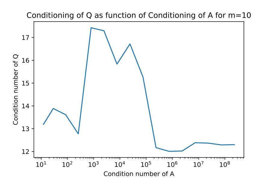 Figure 1
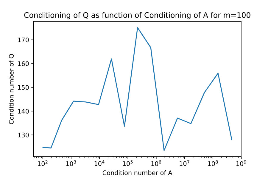 Figure 2
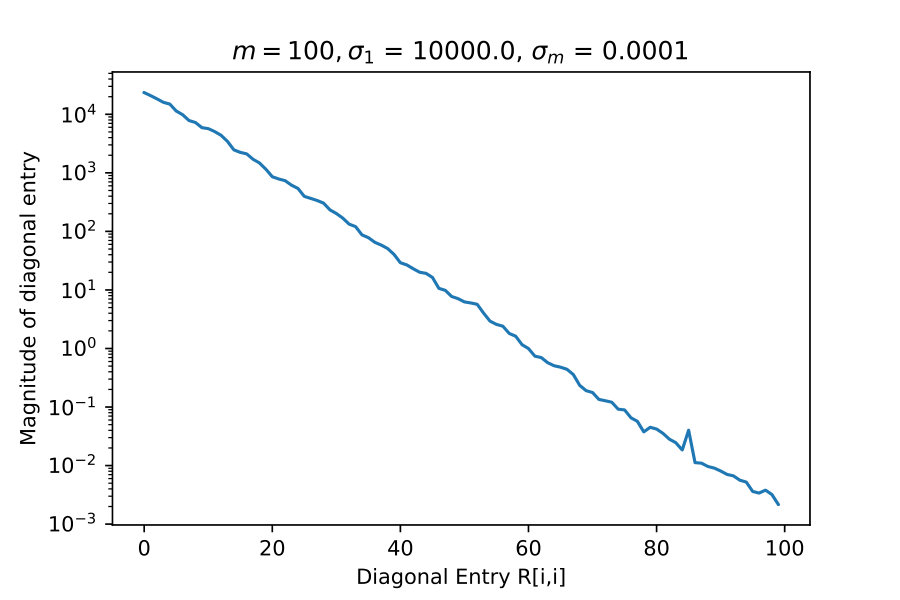 Figure 3
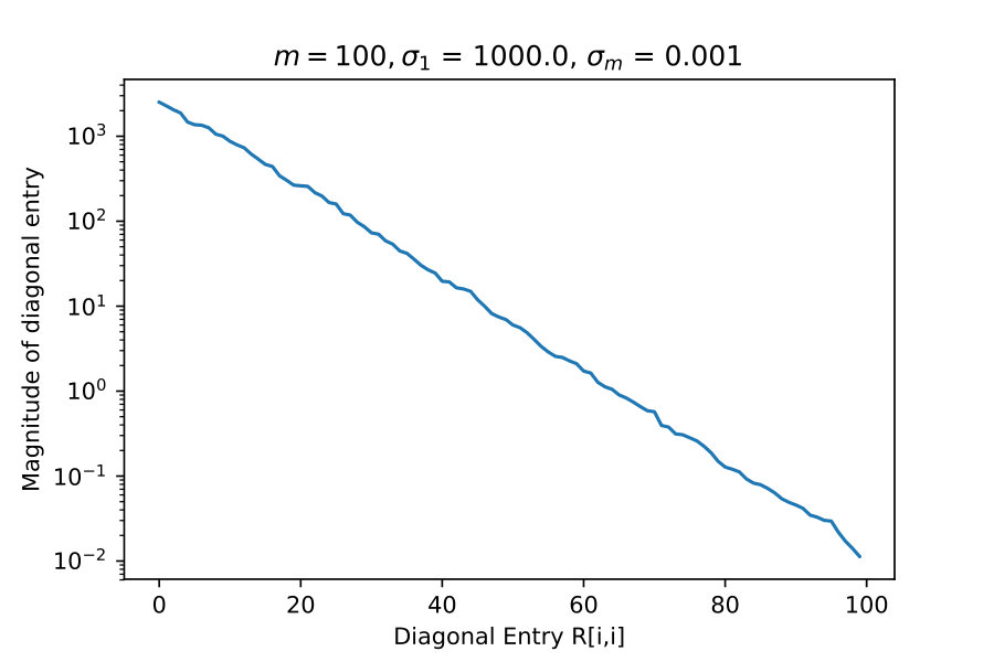 Figure 4
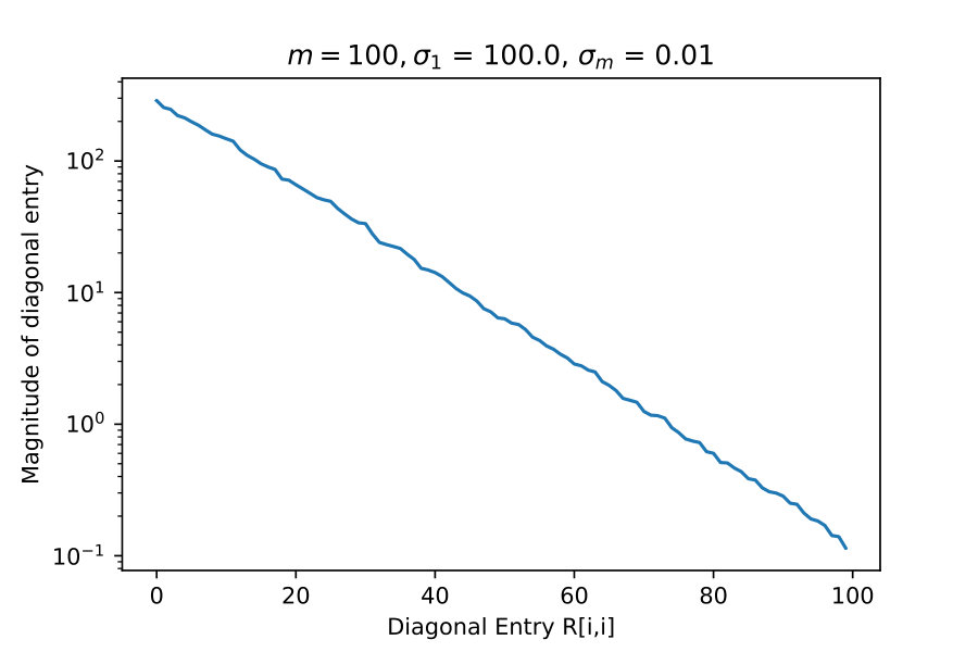 Figure 5
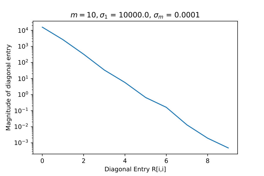 Figure 6
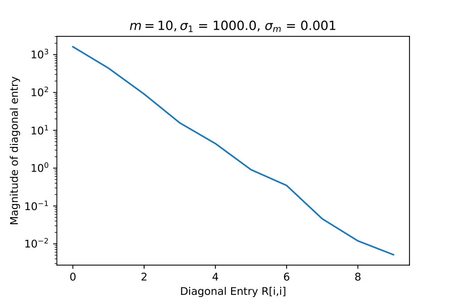 Figure 7
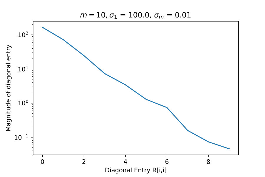 Figure 8
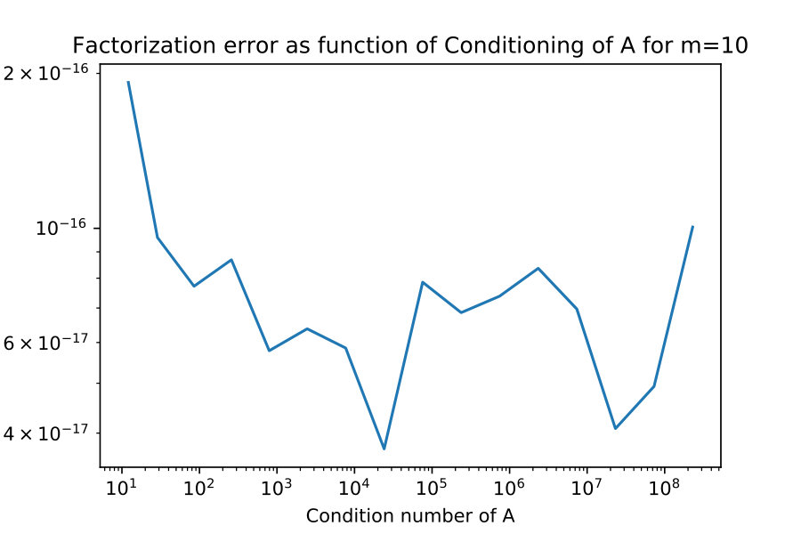 Figure 9
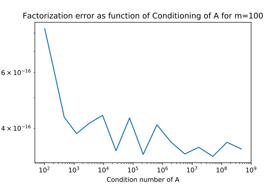 Figure 10
 Figure 1
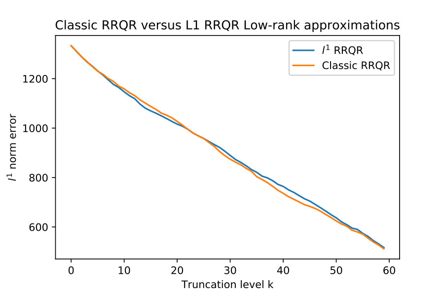 Figure 12
 Figure 13
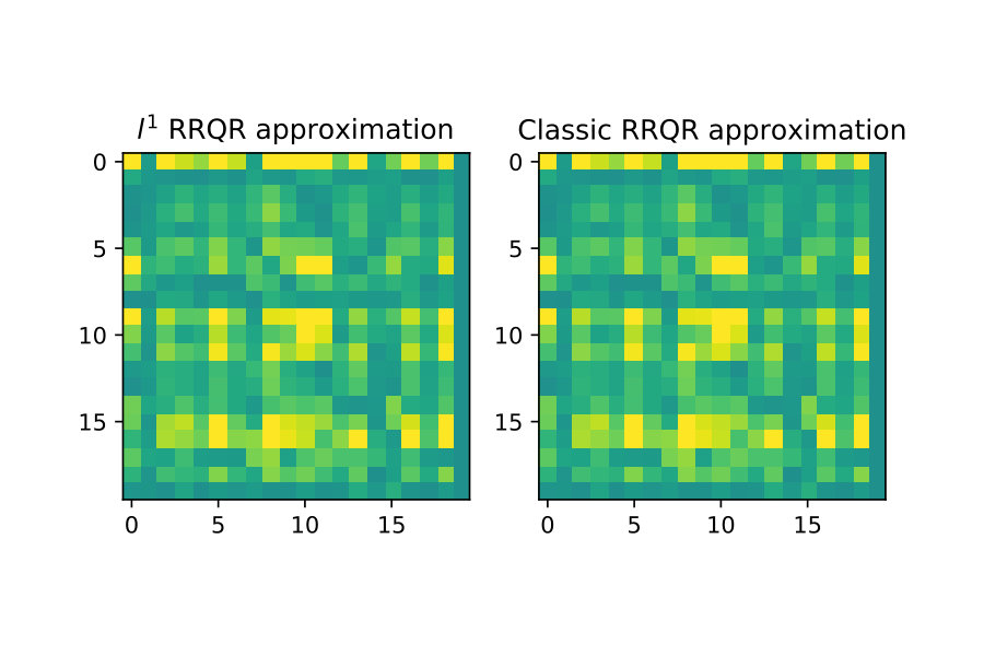 Figure 14
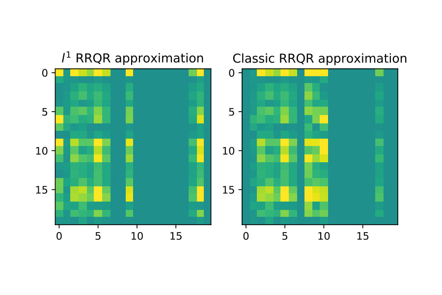 Figure 15
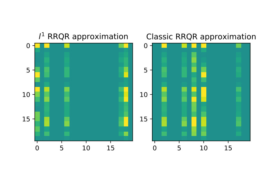 Figure 16
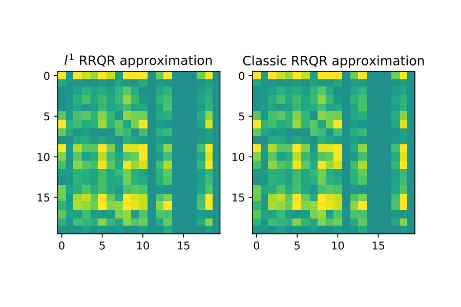 Figure 17
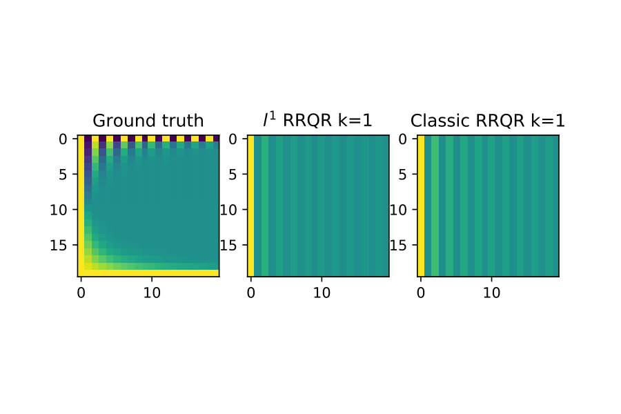 Figure 18
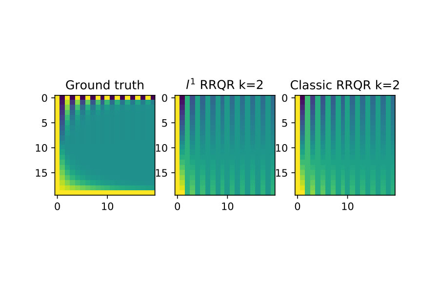 Figure 19
 Figure 20
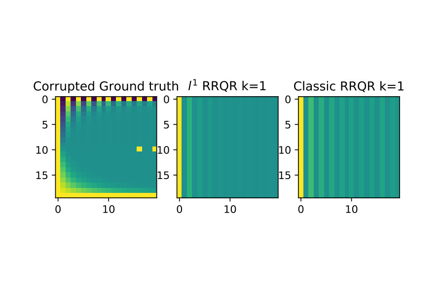 Figure 21
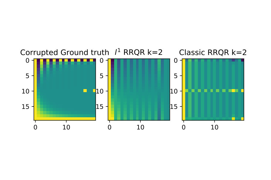 Figure 22
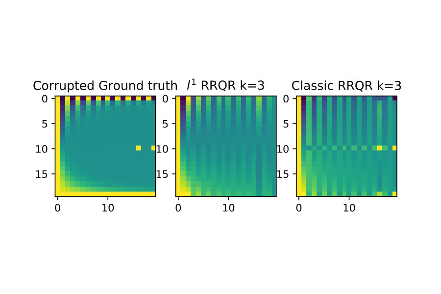 Figure 23
Peer Reviews
No public reviews on file for this paper yet. If you reviewed it on a platform where reviews are public (OpenReview, ICLR, NeurIPS, ICML), you can paste yours below so the community can read it here.
Videos
No videos yet. Explain this paper in a talk, walkthrough, or lecture? Add one.
Taxonomy
TopicsSparse and Compressive Sensing Techniques · Face and Expression Recognition · Image and Signal Denoising Methods
\newsiamremark
remarkRemark \newsiamremarkhypothesisHypothesis
\newsiamthmclaimClaim \headersA Rank Revealing Factorization Using Arbitrary NormsR. Atcheson
A Rank Revealing Factorization Using Arbitrary Norms
Reid Atcheson Numerical Algorithms Group (). [email protected]
Abstract
The classic rank-revealing QR factorization factorizes a matrix as where permutes the columns of , is an orthogonal matrix, and is upper triangular with non-increasing diagonal entries. This is called rank-revealing because careful choice of allows the user to truncate the factorization for a low-rank approximation of with an error term computed in the norm. In this paper I generalize the QR factorization to use any arbitrary norm and prove analogous properties for and in this setting. I then show an application of this algorithm to compute low-rank approximations to with error term in the norm instead of the norm. I provide Python code for the case as demonstration of the idea.
keywords:
QR factorization,rank-revealing QR factorization,low-rank approximation
{AMS}
65F35, 65F30
1 Introduction
Low-rank approximation allows the user to compress an input matrix in a very informative way. The low-rank factors can provide useful information about the data which comprises the input matrix, which forms the basis of Principal Component Analysis (PCA). The gold-standard of low-rank approximations is the SVD factorization, which gives optimal low-rank approximations with respect to the Euclidean norm . The problem with SVD is that algorithms for it typically must be iterative in nature, or even probabalistic. A non-iterative and deterministic algorithm which reveals rank information can therefore be useful.
The rank-revealing QR factorization [2] is a deterministic and non-iterative algorithm which provides rank information on the input matrix by way of the diagonal entries of its upper triangular factor. It turns out this factorization can in fact be used directly for low-rank approximation also, bypassing the SVD entirely, and this has been exploited heavily in areas such as hierarchical compression of matrices [3],[4]. Like with the SVD the quality of this low-rank approximation is often best in the Euclidean norm because the factorization is explicitly based on the Euclidean dot product. This optimality in the Euclidean norm has some undesirable properties in other fields however.
For some applications of data analysis the optimality of a low-rank approximation in the Euclidean norm results in unfavorable low-rank factors, because outliers in data can quickly overwhelm the Euclidean norm of that data, resulting in poor approximations. This has led to the field of ”L1 PCA” which tries to find optimal low rank approximations in the norm instead of the norm [11],[6],[7]. Unfortunately, since the factorization is highly specialized to the Euclidean norm this suggests that rank-revealing strategies can not help in domain. Thus this new area of low-rank approximation has moved in the direction of iterative or probabalistic SVD-like algorithms [7].
In this paper I show that the factorization can be generalized to norms other than the Euclidean norm. I derive the algorithm, state and prove analogous properties of the resulting and factors, and then show numerical results. This yields a deterministic and non-iterative algorithm with rank-revealing properties with the potential to give optimality in norms besides the Euclidean norm.
The paper is organized as follows. The main theory and algorithm is presented in Section 2, an implementation of this algorithm in python for the special case of the norm is in section Section 3, experimental results are in Section 4, and the conclusions follow in Section 5.
2 Main results
I start by presenting the algorithm that this paper is based on. This algorithm accepts a matrix and any norm on and returns a permutation , an upper triangular matrix with nonincreasing diagonal, and such that . I then prove key facts about this algorithm (theorem 2.1) and state a conjecture (conjecture 2.2). I also prove that when the input norm is equal to the Euclidean norm, then the factorization reduces to a classical - in the sense that becomes orthogonal. This is theorem 2.4. I start first with the algorithm 1 below.
The key theoretical result of this paper is summarized in theorem 2.1. Following this theorem is a conjecture which seems true based on numerical evidence supporting it (see section Section 4) but a full proof remains elusive. Finally I prove in theorem 2.4 that if = then algorithm 1 outputs as orthogonal.
Theorem 2.1** (Arbitrary-norm Rank-Revealing factorization ).**
Suppose that , is a norm, and that are output by algorithm 1.
Then the following properties hold:
[TABLE]
[TABLE]
There exists a constant independent of such that
[TABLE]
Conjecture 2.2** (Inverse Bound).**
Suppose that , is a norm, and that are output by algorithm 1.
Then there exists a constant that depends only on the norm such that
[TABLE]
Properties 15 and 16 are standard and precisely match the classical factorization with column pivoting. Properties 17 and 18 perhaps require more explanation. In the classical factorization the matrix is orthogonal (). Strictly speaking we could insist that also be orthogonal in the above theorem, but the utility of orthogonality is lost when using norms different from the norm. This utility stems from the fact that the norm is derived from an inner product, so orthogonality has strong implications on the conditioning of in this norm.
Thus to find an analogue to orthogonality I require that the matrix be well conditioned. The bounds 17 and 18 prove that is invertible (full-rank), but also that the conditioning of does not depend on the conditioning of which the theorem allows to be highly numerically singular. By way of example, if we were to state this theorem for then we would actually have .
I now prove theorem 2.1, minus the conjecture:
Proof 2.3**.**
To prove equation 15 note that follows directly from the base case definitions of these quantities. Now assume for some Then
[TABLE]
For 16 it’s clear that is upper triangular, but to show that its diagonal entries are nonincreasing observe that from the optimality property of we have
[TABLE]
and for any :
[TABLE]
and finally for the conditioning properties 17 and 18 observe that if then
[TABLE]
*where the final inequality is a consequence of Holder’s inequality. Finally we may apply norm equivalence between all norms in finite dimensional spaces to choose such that holds for all to complete the proof of 17. The bound 18 remains conjecture, but is supported by numerical evidence in section Section 4 *
Theorem 2.4** (Classic QR as Special Case ).**
Suppose that , is the norm, and that are output by algorithm 1.
*Then is orthogonal, i.e. . *
Proof 2.5**.**
By the inductive definition of in 8 we have
[TABLE]
Recall that solves the minimization problem
[TABLE]
*which means it is forming the projection of onto the space . Since is the residual of this projection, it is orthogonal to the whole space . *
3 Implementation for norm using linear programming
The key ingredient of algorithm 1 is the ability to compute solutions to minimum-norm linear problems such as . For the case there are already established and robust algorithms for this problem, but it’s less obvious for other norms. For the norm we can cast it as a linear program. In other words:
[TABLE]
is equivalent to the linear program
[TABLE]
This is implemented using Python in the appendix at listing 8, this uses the open source tools NumPy [12] and SciPy [5].
The linear program approach is correct but does not seem to scale well for larger matrices Thus I also provide a Python implementation that uses the NAG numerical library [9] in listing 9. Furthermore I have also implemented the relations 4 and 8 as a function in python in listing 10. This implementation can use either the NAG solver from 9 or the open source solver from 8 by changing the value of the l1alg parameter.
I now proceed to show numerical results of this algorithm.
4 Experimental results
The results below are designed to validate some of the theoretical properties proven and asserted earlier. These include properties like the well-conditioning of and the non-increasing property for the diagonal of . I also include results on low-rank approximation from this factorization as that was the primary motivation of deriving this algorithm.
4.1 Diagonal Entries of R
These experiments test the theorem result 16. Here I take constructed explicitly as an SVD factorization with diagonal entries of varying in relative size, which I indicate with and .
If truly has rank-revealing properties then it should exhibit rapid decay of diagonal entries when becomes progressively more singular.
These results suggest that is capturing low rank information.
4.2 Conditioning of Q
An important part of successful rank-revealing factorization is the conditioning of should be independent of the conditioning of . The key theoretical result which would prove this would be 18, but unfortunately I was unable to prove this. Here I give numerical evidence that it does appear to be true.
I take constructed explicitly as an SVD factorization with diagonal entries of varying in relative size. I compute the condition numbers , and plot them against each other in figure 3.
4.3 Factorization error
Next I illustrate that the factorization error also does not depend on the conditioning of .
I take constructed explicitly as an SVD factorization with diagonal entries of varying in relative size. I compute the condition numbers , and factorization errors and plot them against each other in figure 4
4.4 Low-rank approximation
With the rank-revealing properties validated I now show an example of low-rank approximation.
For this test I again generate by forming it as an explicit SVD factorization with and . I then compute two factorizations of :
[TABLE]
Next I truncate the factorizations to be a rank- approximation to as follows:
[TABLE]
For the first study I compare the induced matrix norm error of these approximations for this is in figure 5.
This result suggests that there is little difference in results between and rank revealing factorizations. The next section 4.5 shows the subtle difference between and norms for low-rank approximations, and why the norm may be preferred in some situations.
4.5 Resistance of norm to outliers
One of the original motivations for deriving algorithm 1 was to be able to do low-rank approximations, which can be very robust with respect to outliers in data [1].
I show here that to some extent this appears to be reflected in the version of the rank revealing factorization. To illustrate this I first show a ”clean” example without outliers, and then do rank approximations for for both classical RRQR and RRQR. Then I introduce outliers to this same data and show the classical RRQR algorithm quickly is drawn to over-resolve outlier data because of how it dominates the Euclidean norm.
The first case are the low-rank approximations without outliers in the input data
The next case I introduce two outliers of much larger magnitude than surrounding data. The classical RRQR quickly gravitates to the columns containing these outliers because the outlier data gets squared in the Euclidean norm and then dominates it. In the norm however this effect is much less pronounced. See figure 7 below.
5 Conclusions
I derived a rank-revealing factorization that shares some similarities to classic rank-revealing QR with column pivoting. Instead of the factor being orthogonal it has conditioning that is independent of the conditioning of . Furthermore the rank-revealing factorization presented here does not depend strictly on using dot products and the norm. I validated that claim by implementing the algorithm for the norm case, where least-norm-solution is equivalent to a linear program.
While I was able to numerically validate the conditioning properties of I was unable to mathematically prove them. The key fact to be proven remains conjecture (2.2). Without orthogonality properties available in the case most avenues for proof are lost. I believe however that careful use of the optimality properties for the least-norm solution (see eqns 8) may be able to overcome the loss of orthogonality.
Appendix A Python Implementations
This section contains python implementations for the key algorithms of this paper. I give three implementations here. The first two, implementations 8 and 9 solve the same problem, and may be used interchangeably in the following implementation 10 which actually computes the rank-revealing factorization.
The first algorithm solves linear systems in the least--norm sense by translating it to a linear program and then using SciPy. This has the advantage of only requiring open source tools that are readily available on the internet.
The next Python implementation makes use of the NAG library routine e02ga through the Nag Library for Python [8]. Full documentation for this routine may be found at [10]. This relies on the closed-source NAG library, but since the e02ga routine is specialized to the least--norm problem it is significantly faster than a generic linear-programming approach as shown above. This is important for the rank revealing factorization because it spends almost all of its time solving linear systems in this minimum-norm sense. This enables factorizing much larger matrices.
Finally the actual factorization. As mentioned above, this factorization depends on the ability to solve linear systems in the least-norm sense. Since I gave two possible ways to achieve this, I made the least-norm-solver an input argument which may be changed either to the fully open source solver, or to the faster NAG-based solver.
The reference list from the paper itself. Each links out to its DOI / PubMed record.
- 1[1] E. J. Candès, X. Li, Y. Ma, and J. Wright , Robust Principal Component Analysis? , J. ACM, 58 (2011), pp. 11:1–11:37, https://doi.org/10.1145/1970392.1970395 , http://doi.acm.org/10.1145/1970392.1970395 (accessed 2019-05-04). · doi ↗
- 2[2] T. F. Chan , Rank revealing QR factorizations , Linear Algebra and its Applications, 88-89 (1987), pp. 67–82, https://doi.org/10.1016/0024-3795(87)90103-0 , http://www.sciencedirect.com/science/article/pii/0024379587901030 (accessed 2019-05-05). · doi ↗
- 3[3] W. Hackbusch , A Sparse Matrix Arithmetic Based on $\Cal H$-Matrices. Part I: Introduction to $ { \Cal H } $-Matrices , Computing, 62 (1999), pp. 89–108, https://doi.org/10.1007/s 006070050015 , https://doi.org/10.1007/s 006070050015 (accessed 2019-05-06). · doi ↗
- 4[4] W. Hackbusch, L. Grasedyck, and S. Börm , An introduction to hierarchical matrices , Mathematica Bohemica, v.127, 229-241 (2002), 127 (2002).
- 5[5] E. Jones, T. Oliphant, P. Peterson, and others , Sci Py: Open source scientific tools for Python , 2001, http://www.scipy.org/ .
- 6[6] P. P. Markopoulos, S. Kundu, S. Chamadia, and D. A. Pados , Efficient L 1-Norm Principal-Component Analysis via Bit Flipping , IEEE Transactions on Signal Processing, 65 (2017), pp. 4252–4264, https://doi.org/10.1109/TSP.2017.2708023 , http://arxiv.org/abs/1610.01959 (accessed 2019-04-28). ar Xiv: 1610.01959. · doi ↗
- 7[7] P. P. Markopoulos, S. Kundu, S. Chamadia, N. Tsagkarakis, and D. A. Pados , Outlier-Resistant Data Processing with L 1-Norm Principal Component Analysis , in Advances in Principal Component Analysis: Research and Development, G. R. Naik, ed., Springer Singapore, Singapore, 2018, pp. 121–135, https://doi.org/10.1007/978-981-10-6704-4_6 , https://doi.org/10.1007/978-981-10-6704-4_6 (accessed 2019-05-04). · doi ↗
- 8[8] The Numerical Algorithms Group (NAG) , The nag library , www.nag.com .