PRSim: Sublinear Time SimRank Computation on Large Power-Law Graphs
Zhewei Wei, Xiaodong He, Xiaokui Xiao, Sibo Wang, Yu Liu, Xiaoyong Du,, Ji-Rong Wen

TL;DR
PRSim introduces a sublinear time algorithm for single-source SimRank queries on large power-law graphs, enabling efficient real-time similarity computations with high accuracy and small index size.
Contribution
The paper presents PRSim, a novel algorithm that exploits graph structure to achieve sublinear query time for SimRank, with theoretical guarantees and superior empirical performance.
Findings
PRSim achieves sublinear query time on power-law graphs.
PRSim outperforms existing algorithms in speed and accuracy.
The empirical analysis confirms the theoretical advantages of PRSim.
Abstract
{\it SimRank} is a classic measure of the similarities of nodes in a graph. Given a node in graph , a {\em single-source SimRank query} returns the SimRank similarities between node and each node . This type of queries has numerous applications in web search and social networks analysis, such as link prediction, web mining, and spam detection. Existing methods for single-source SimRank queries, however, incur query cost at least linear to the number of nodes , which renders them inapplicable for real-time and interactive analysis. { This paper proposes \prsim, an algorithm that exploits the structure of graphs to efficiently answer single-source SimRank queries. \prsim uses an index of size , where is the number of edges in the graph, and guarantees a query time that depends on the {\em reverse PageRank} distribution of the input…
Click any figure to enlarge with its caption.
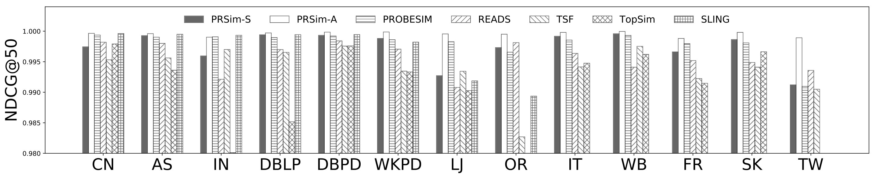 Figure 1
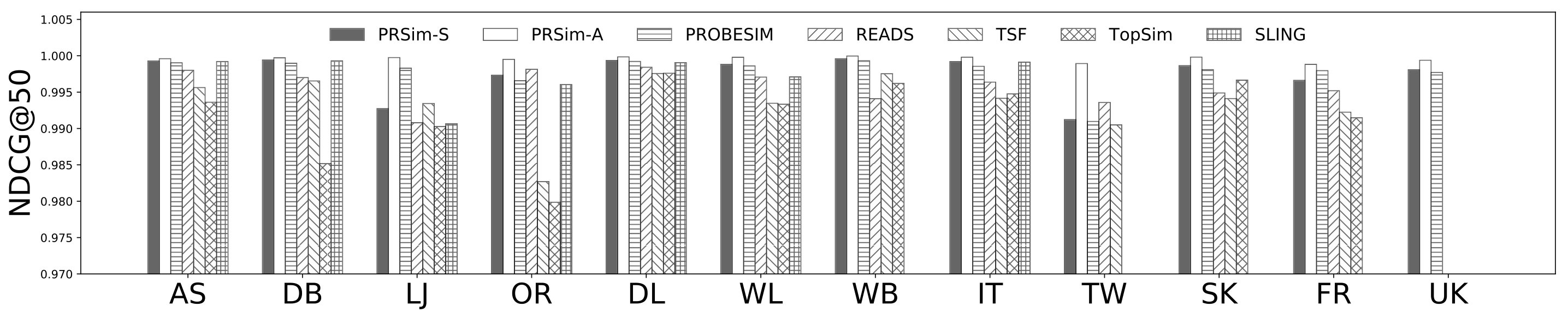 Figure 2
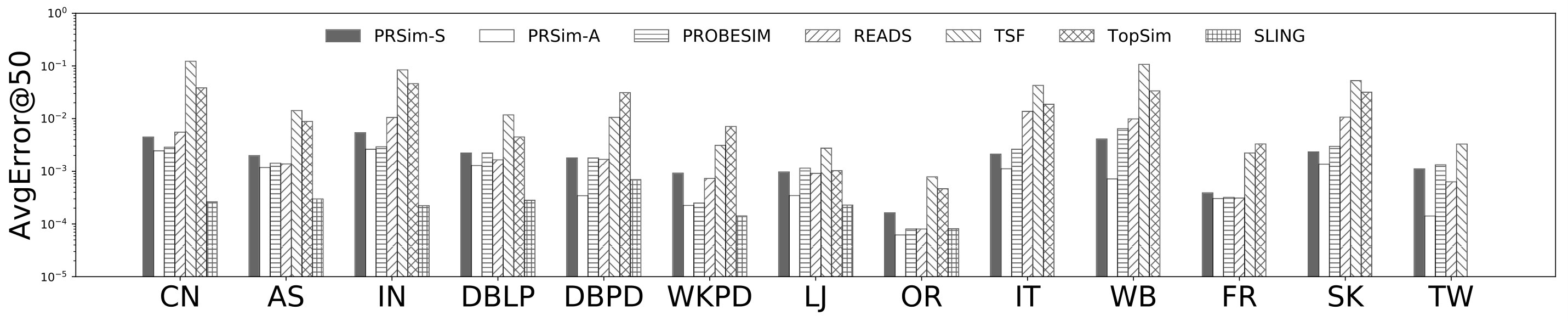 Figure 3
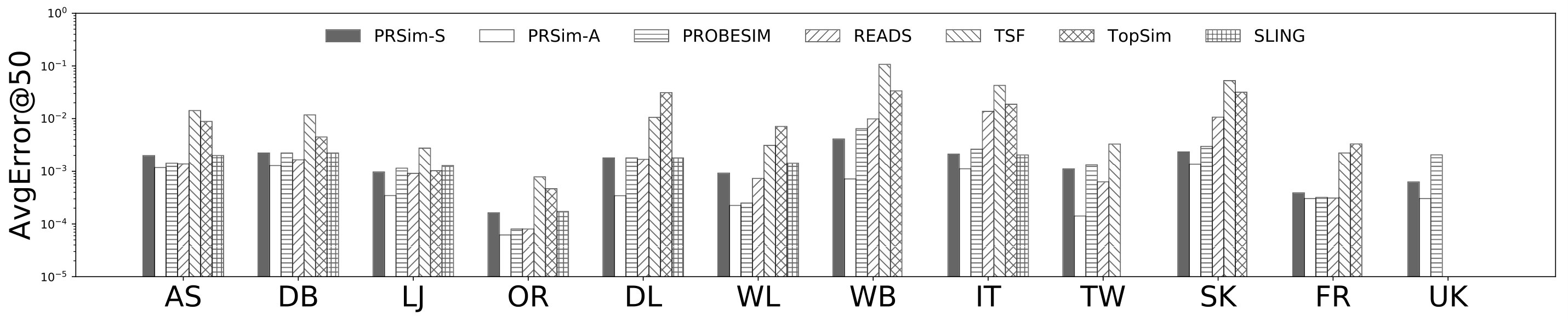 Figure 4
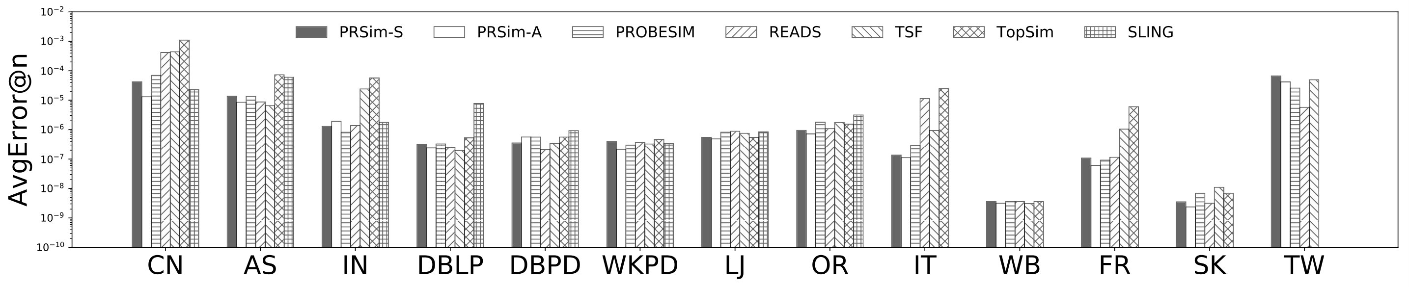 Figure 5
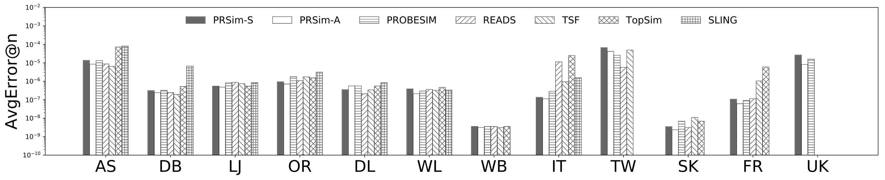 Figure 6
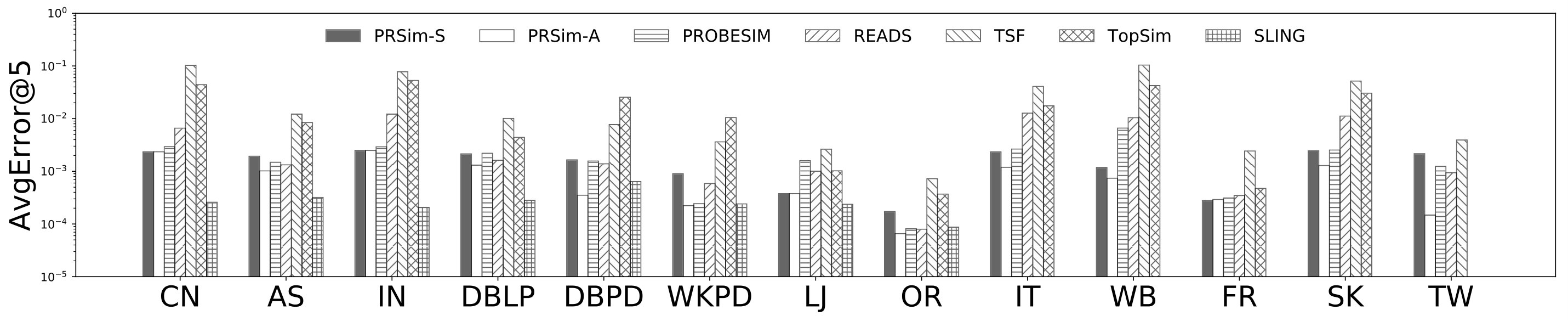 Figure 7
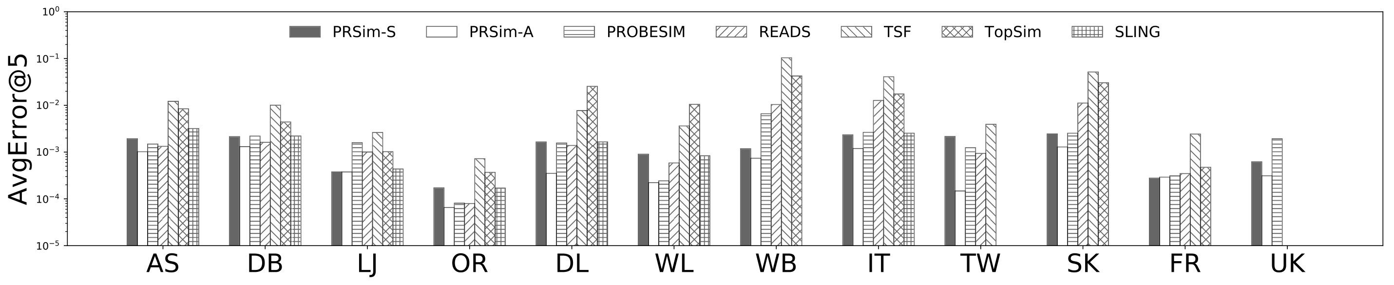 Figure 8
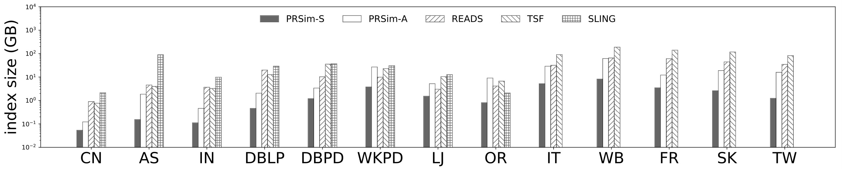 Figure 9
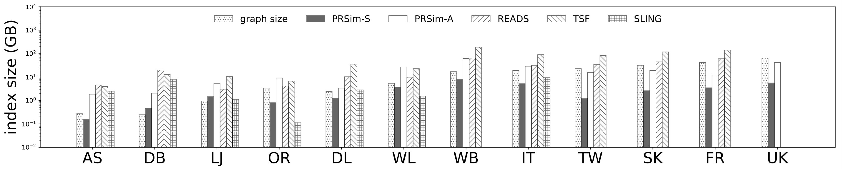 Figure 10
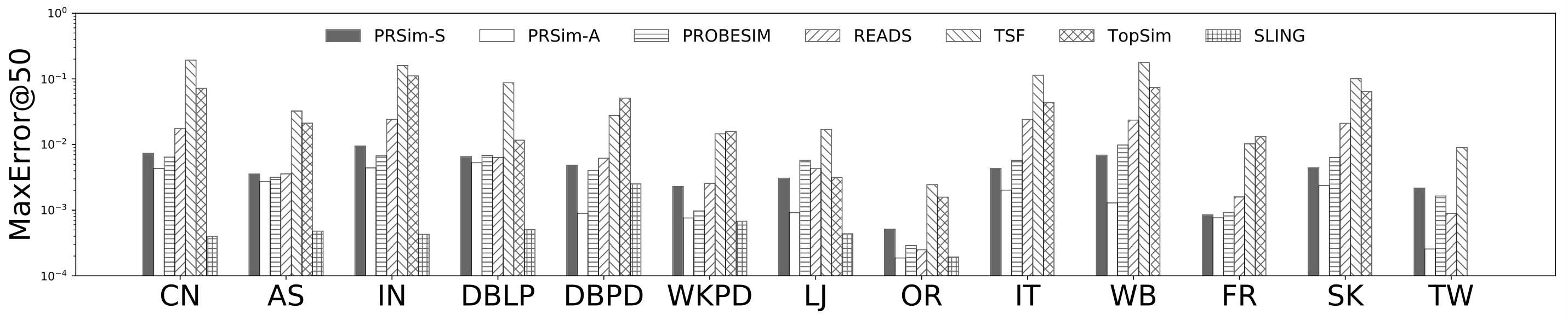 Figure 11
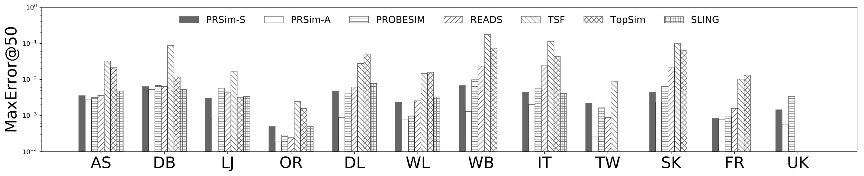 Figure 12
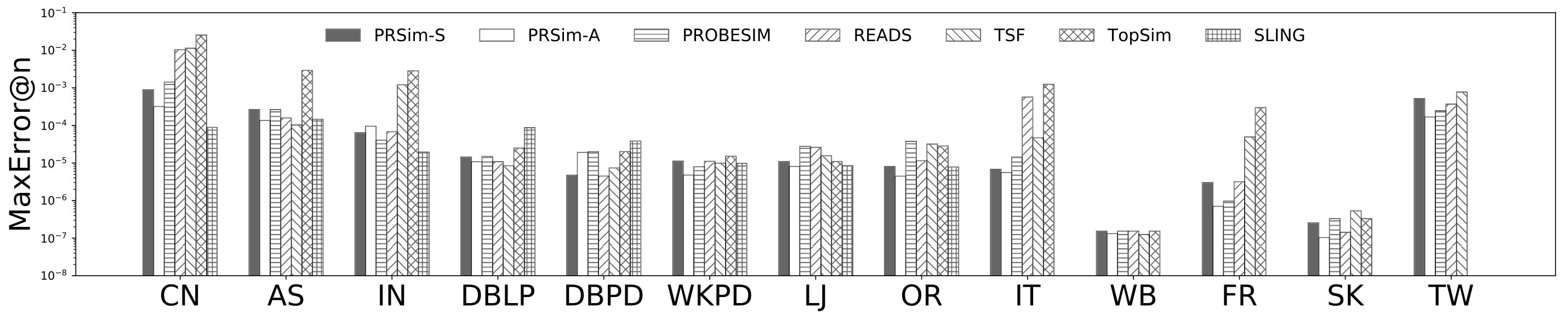 Figure 13
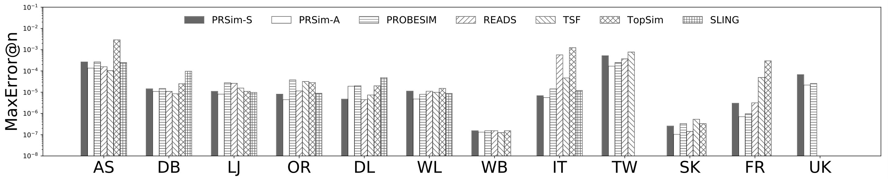 Figure 14
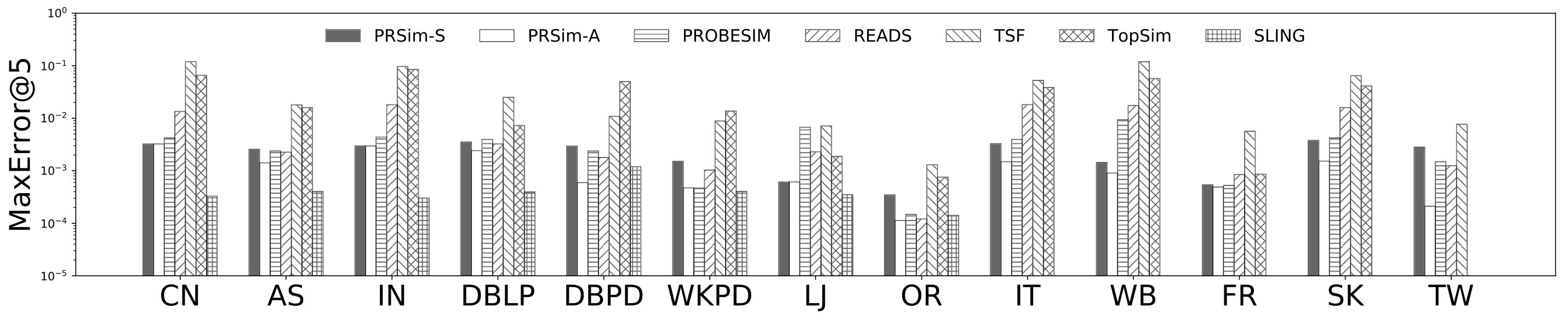 Figure 15
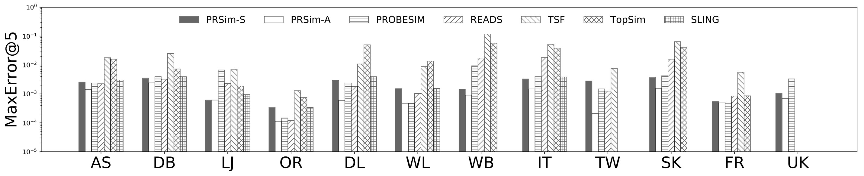 Figure 16
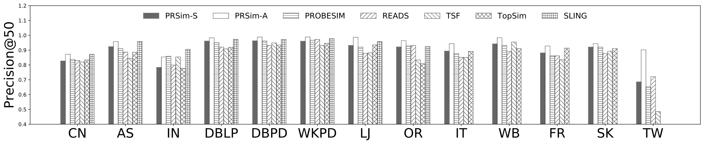 Figure 17
 Figure 18
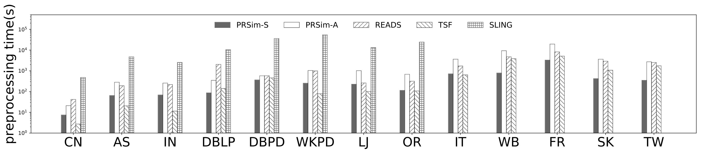 Figure 19
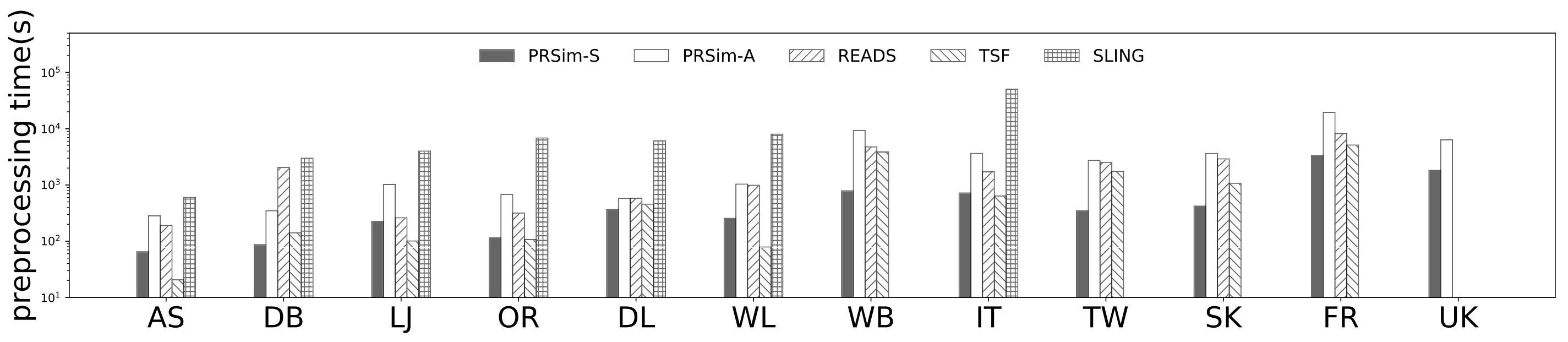 Figure 20
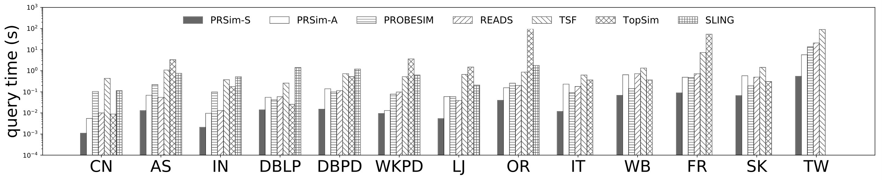 Figure 21
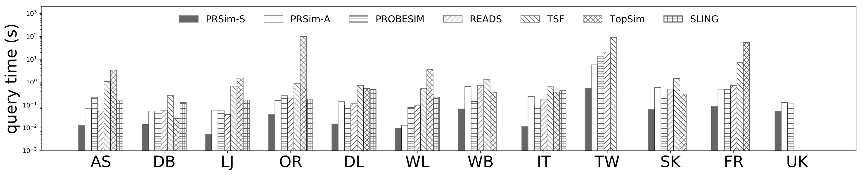 Figure 22
| Algorithm | Query Time | Query Time (Power-Law Graphs) | Space Overhead | Preprocessing Time | |
| PRSim | for | ||||
| for | |||||
| for | |||||
| TSF (SLX15, ) | |||||
| READS (jiang2017reads, ) | |||||
| ProbeSim (liu2017probesim, ) | 0 | 0 | |||
| SLING (TX16, ) | |||||
| Notation | Description |
| the numbers of nodes and edges in | |
| the set of in-neighbors and out-neighbors of a node | |
| , | the out-degree and in-degree of node |
| the SimRank similarity of nodes and | |
| an estimation of | |
| the decay factor of SimRank | |
| the maximum absolute error allowed in SimRank computation | |
| the reverse PageRank of node | |
| the RPPR and -hop RPPR values of with respect to | |
| estimators of and | |
| , | the residue and reserve of at level from in the backward search |
| Data Set | Type | ||
| DBLP-Author (DB) | undirected | 5,425,963 | 17,298,033 |
| LiveJournal (LJ) | directed | 4,847,571 | 68,993,773 |
| It-2004 (IT) | directed | 41,291,594 | 1,150,725,436 |
| Twitter (TW) | directed | 41,652,230 | 1,468,365,182 |
| UK-Union (UK) | directed | 133,633,040 | 5,507,679,822 |
Peer Reviews
No public reviews on file for this paper yet. If you reviewed it on a platform where reviews are public (OpenReview, ICLR, NeurIPS, ICML), you can paste yours below so the community can read it here.
Videos
No videos yet. Explain this paper in a talk, walkthrough, or lecture? Add one.
PRSim: Sublinear Time SimRank Computation on Large Power-Law Graphs
[Technical Report]
Zhewei Wei
School of Information, DEKE MOE, Renmin University of China
,
Xiaodong He
4Paradigm Inc.BeijingChina
,
Xiaokui Xiao
School of Computing, National University of Singapore
,
Sibo Wang
The Chinese University of Hong Kong
,
Yu Liu
Peking University
,
Xiaoyong Du
and
Ji-Rong Wen
Renmin University of China
(2019)
Abstract.
SimRank is a classic measure of the similarities of nodes in a graph. Given a node in graph , a single-source SimRank query returns the SimRank similarities between node and each node . This type of queries has numerous applications in web search and social networks analysis, such as link prediction, web mining, and spam detection. Existing methods for single-source SimRank queries, however, incur query cost at least linear to the number of nodes , which renders them inapplicable for real-time and interactive analysis.
This paper proposes PRSim, an algorithm that exploits the structure of graphs to efficiently answer single-source SimRank queries. PRSim uses an index of size , where is the number of edges in the graph, and guarantees a query time that depends on the reverse PageRank distribution of the input graph. In particular, we prove that PRSim runs in sub-linear time if the degree distribution of the input graph follows the power-law distribution, a property possessed by many real-world graphs. Based on the theoretical analysis, we show that the empirical query time of all existing SimRank algorithms also depends on the reverse PageRank distribution of the graph. Finally, we present the first experimental study that evaluates the absolute errors of various SimRank algorithms on large graphs, and we show that PRSim outperforms the state of the art in terms of query time, accuracy, index size, and scalability.
SimRank; Power-Law Graphs; Personalized PageRank
††journalyear: 2019††copyright: acmcopyright††conference: 2019 International Conference on Management of Data; June 30-July 5, 2019; Amsterdam, Netherlands††booktitle: 2019 International Conference on Management of Data (SIGMOD ’19), June 30-July 5, 2019, Amsterdam, Netherlands††price: 15.00††doi: 10.1145/3299869.3319873††isbn: 978-1-4503-5643-5/19/06††ccs: Mathematics of computing Graph algorithms††ccs: Information systems Data mining
1. Introduction
Measuring similarities and proximities of nodes in the graph is a classic task in graph analytics. Several link-based similarity measures have been proposed, including Personalized PageRank (page1999pagerank, ), Simfusion (xi2005simfusion, ), P-rank (zhao2009p, ) and Panther (zhang2015panther, ). Among them, SimRank (JW02, ), proposed by Jeh and Widom, is regarded as one of the most influential similarity measures, and has been adopted in numerous applications such as web mining (Jin11, ), social network analysis (NK07, ), and spam detection (SH11, ). Given a graph , the SimRank similarity of nodes and , denoted as , is defined as
[TABLE]
where denotes the set of in-neighbors of , and is a decay factor typically set to 0.6 or 0.8 (JW02, ; LVGT10, ). This formulation is based on two intuitive statements: (1) two objects are similar if they are referenced by similar objects, and (2) an object is most similar to itself. Due to its recursive nature, SimRank computation is a non-trivial problem and has been extensively studied for more than a decade. Existing work mostly considers three types of SimRank queries: (1) Single-pair queries, which ask for the SimRank similarity between two given nodes and ; (2) All-pair queries, which ask for the SimRank similarity between any pair of nodes and ; (3) Single-source queries, which ask for the SimRank similarity between every node and . All-pair queries require storing node pairs, and thus is infeasible for large graphs. Meanwhile, single-source queries has become the focus of recent research (KMK14, ; MKK14, ; TX16, ; FRCS05, ; LeeLY12, ; LiFL15, ; SLX15, ; YuM15b, ; LiFL15, ; jiang2017reads, ; liu2017probesim, ), due to its connections to recommendation applications. In this paper, we aim to answer approximate single-source SimRank queries, defined as follows:
Definition 1.1 (Approximate Single-Source Queries).
Given a node in a directed graph and an absolute error threshold , an approximate single-source SimRank query returns an estimated value for each node in , such that
[TABLE]
holds for any with at least probability.
Power-law graphs. It was experimentally observed that most real-world networks are scale-free and follow power-law degree distribution. In particular, let and denote the fraction of nodes in the graph having out-degree and in-degree at least , respectively. Then, on a power-law graph, and satisfy that and (BollobasBCR03, ), where and are the (cumulative) power-law exponents that usually take values from to . Recent work has demonstrated that by exploiting this fact, we can improve the asymptotic bounds for various graph algorithms such as triangle counting (brach2016algorithmic, ), transitive closure (brach2016algorithmic, ), perfect matching (brach2016algorithmic, ), PageRank computation (lofgren2015personalized, ; wei2018topppr, ) and maximum independent set (liu2015towards, ).
Motivations. Since many graph algorithms can benefit from the structure of real-world graphs, a natural question is: Can we do the same for SimRank algorithms? On one hand, we are interested in designing a more efficient SimRank algorithm by exploiting the structure of the graphs, since existing work for SimRank computation (KMK14, ; MKK14, ; TX16, ; FRCS05, ; LeeLY12, ; LiFL15, ; SLX15, ; YuM15b, ; LiFL15, ; jiang2017reads, ; liu2017probesim, ) has missed this opportunity for optimization.
On the other hand, we are also interested in analyzing how the graph structure affects the performance of existing SimRank algorithms. More precisely, it has been observed in previous work (zhangexperimental, ) that the performance of existing SimRank algorithms may vary dramatically on graphs with similar numbers of nodes and edges. A typical example is the Twitter (TW) and IT-2004 (IT) data sets, both of which have around 40 million nodes and 1 billion edges. However, as shown in (zhangexperimental, ) and in our experiments, the query times of most SimRank algorithms are significantly smaller on IT-2004 than on Twitter. Based on this phenomenon, (zhangexperimental, ) suggests that Twitter (TW) is “locally dense” and IT-2004 (IT) is “locally sparse”. However, it is still desirable to obtain a quantifiable measure that describes the hardness of each graph in terms of SimRank computation. Finally, since obtaining ground truth for single-source SimRank queries requires space, which is infeasible for large graphs, most existing work only evaluate the accuracy of the algorithms on small graphs. The only exception is recent work (liu2017probesim, ), which evaluates precision for approximate top- queries on graphs with billion edges using the idea of pooling. However, there is no prior experimental study that evaluates absolute error for single-source queries on large graphs.
Our contributions. This paper studies the approximate single-source SimRank queries, and makes the following contributions.
(1) We propose PRSim, an algorithm that leverages the graph structure to efficiently answer approximate single-source SimRank queries. The query time complexity of PRSim is related to the reverse PageRank of the input graph , which is defined as the PageRank of the graph constructed by reversing the direction of each edge in . Let denote reverse PageRank of node , and denote the second moment of the reverse PageRanks. The average expected query cost for PRSim on worst-case graphs is bounded by . By the fact that , PRSim provides at least the same complexity as the random walk based algorithms (ProbeSim, TSF, and READS) do on worst-case graphs. Furthermore, PRSim uses an index of size , which significantly improves the scalability of the algorithm. See Table 1 for the theoretical comparison between our algorithm and the state of the art.
On the other hand, we show that on power-law graphs, the second moment is an asymptotic variable that is close to [math], which means PRSim actually achieves sub-linear query cost on real-world graphs. More precisely, Let denote the cumulative power-law exponent of the out-degree distribution. We show that the average expected query cost for PRSim on power-law graphs is bounded by:
[TABLE]
for and . To understand this complexity, we first note that when , our bounds depend only on , which is significantly better than the corresponding bound of any previous SimRank algorithms. For , since , we have . This implies that PRSim also outperforms SLING on power-law graphs. To the best of our knowledge, this is the first sublinear algorithm for single-source SimRank queries on power-law graphs.
(2) To achieve the desired query cost in Table 1, we design several novel techniques for computing SimRank and Personalized PageRank (PPR) . First, we propose an algorithm that estimates the last meeting probabilities (TX16, ) (see Section for definition) for ALL nodes in time. This improves the bounds in (TX16, ) by an order of and is the key to achieve sub-linearity. Second, we propose an index scheme which performs the backward search (lofgren2015personalized, ) algorithm only on a number of hub nodes. The parameter enables us to manipulate the tradeoffs between index size and query time, which improves the scalability of our algorithm. Finally, we design Variance Bounded Backward Walk, an algorithm that estimates the Personalized PageRank values to a given target node with additive error in time, where is the reverse PageRank of node . Since the average value of is , this significantly improves the time complexity of the Randomized Probe algorithm (liu2017probesim, ), and is the key to the relation between the time complexity and the reverse PageRank distribution. We also note that the Variance Bounded Backward Walk algorithm actually improves the time complexity of state-of-the-art PPR algorithms to target nodes for dense graphs (wang2018efficient, ), and may be of independent interest.
(3) Based on the time complexity of PRSim, we conduct experiments to confirm that the hardness of SimRank queries is indeed reversely related to the out-degree power-law exponent of the graph. This observation provides a quantifiable measure for the concept of locally dense and locally sparse networks introduced in (zhangexperimental, ). In particular, the out-degree distribution of IT-2004 is significantly more skewed than that of Twitter (see Figure 1), which explains the performance discrepancy of existing SimRank algorithms on these two datasets. We also conduct a large set of experiments that evaluate PRSim against the state of the art on benchmark data sets. In particular, our experiments include the first empirical study on the tradeoffs between absolute error and query cost for single-source SimRank algorithms on graphs with billions of edges. Our empirical study shows that PRSim outperforms the state of the art in terms of query time, accuracy, index size, and scalability.
2. Preliminaries
Table 2 shows the notations that are frequently used in the remainder of the paper.
-walk and Reverse PageRank. We unify the definition of SimRank and reverse PageRank under the notation of -walk. Let be a directed graph with nodes and edges. Given a source node and a decay factor , a reverse -discounted random walk (or -walk in short) from is a traversal of that starts from and, at each step, either (i) terminates at the current node with probability, or (ii) proceeds to a randomly selected in-neighbor of the current node with probability. We define the reverse PageRank of a node to be the probability that an -walk from a uniformly chosen source node terminates at . It is easy to see that the reverse PageRank of a node in the original graph equals to the PageRank of in the reverse graph constructed by reversing the direction of each edge in .
Given a source node and a target node , we further define the reverse Personalized PageRank (RPPR) of with respect to to be the probability that an -walk from terminates at . Again, the reverse Personalized PageRank on the original graph equals to the Personalized PageRank on the reverse graph . Since the RPPR values from a given source node form a probability distribution, we have Meanwhile, since the reverse PageRank is equal to the probability that an -walk from a random source node terminates at , we have
-Hop RPPR. In this paper, we will mainly use a variant of Personalized PageRank called -hop Reverse Personalized PageRank (-hop RPPR). Given a source node , the -hop RPPR of node respected to is the probability that a reverse -walk from terminates at node with exactly steps. By the definition of -hop RPPR, we have
[TABLE]
On the other hand, it is easy to see that RPPR can be expressed as the sum of -hop RPPR, that is, Thus, we have and
[TABLE]
SimRank, -walk, and hitting probability. It is shown in (TX16, ) that the SimRank similarity between two different nodes and can also be formulated using -walks. Given two distinct nodes and , we start a -walk from each node. If the two -walks visit the same node after exactly steps, we say the two -walks meet at step . (TX16, ) shows that is equal to the probability that the two -walks meet.
Moreover, (TX16, ) proposes SLING, an algorithm that uses the following formula to estimate SimRank values:
[TABLE]
Here denote the hitting probability that an -walk from node visits in its -step, and is a parameter that characterizes the last-meeting probability:
Definition 2.1 (Last-meeting probability).
The last-meeting probability for node is the probability that two -walk from do not meet at step for any .
SLING precomputes and with an additive error up to , and stores them in the index. Given a query node , it retrieves all levels and nodes such that . For each pair, SLING retrieves all nodes with and , and estimates with Equation (5).
There are two major issues with SLING. First, storing all with additive error up to takes space, which can be significantly larger than the graph size for reasonable choices of . Second, approximating for each requires sampling a large number of random walks from each node in the graph, which makes the preprocessing time infeasible on very large graphs. Our algorithm overcomes these two drawbacks by (1) providing an index size that is at most the size of the graph, and (2) designing an algorithm that estimates on-the-fly, using only time.
3. PRSim algorithm
In this section, we present PRSim, an index-based algorithm that exploits the graph structure to efficiently answer approximate single-source SimRank queries. We first provide the estimating formula that relates SimRank and -hop RPPR.
3.1. SimRank and -hop RPPR
The relation between SimRank and reverse Personalized PageRank can be directly derived from equation (5). Observe the fact that -hop RPPR equals to the hitting probability multiplied the the termination probability , and we have
[TABLE]
There are two reasons for using -hop RPPR over hitting probability. Firstly, we have . As we will show later, this is critical for estimating in time. Secondly, we have . This property relates SimRank with the reverse PageRank, and thus is essential for achieving sublinear query time.
Recall that given a source node , our goal is to estimate SimRank values with additive error for any node . By Equation (6), we can decompose the query process into three subroutines: 1) Given a source node , compute the -hop RPPR values for any nodes ; 2) Compute last meeting probabilities for each ; 3) For any node , compute -hop RPPR values to any target node . For the first task, we can employ a simple Monte Carlo algorithm which generates a number of -walks from and uses the proportion of -walks that terminate at with exact steps to approximate . This algorithm runs in time, so we will focus on the remaining two tasks.
3.2. Computing Last Meeting Probability
The first challenge is how to estimate for each efficiently. SLING (TX16, ) generates pair of -walks for each , and obtains an approximation to with error for each . However, this solution leads to a preprocessing time of , and thus, is not feasible if we need small error on large graphs.
Our first key insight is that, instead of estimating the -hop PPR and last meeting probability separately, we can estimate their product in the query phase, using only samples. More precisely, we observe that is the probability that an -walk from terminates at with steps, and then, two independent -walks from do not meet. Therefore, we can generate an -walk from , and then two -walks and from the node where terminates. If and do not meet, we set the estimator . This way we obtain an unbiased estimator for each , and . We also note that the summation , which means we can use Chernoff bound A.1 to estimates with additive error for any with only samples.
3.3. Precomputing RPPR to Hub Nodes
Given a target node , computing -hop RPPR for any node is time-consuming, especially when is a hub node with many out-neighbors. Therefore, we will use index to help reduce the cost. SLING (TX16, ) proposes the following approach: for each (source) node , we precompute for any and put into an inverted list, so we can efficiently track for a given target node . This approach, however, essentially builds an index for every target node and results in an index of size , which is usually significantly larger than the graph size for reasonably small .
To reduce the index size, we propose to build index only for hub nodes. In particular, we identify nodes with the largest reverse PageRanks as hub nodes, where is a user-specified parameter. We then perform the backward search (lofgren2015personalized, ) algorithm on each hub node to precompute for any and any . The definition of hub nodes is based on two intuitions. First, recall that the reverse PageRank of node is the probability that an -walk from a random node terminates at . Therefore, a hub node is more likely to be visited in a single-source SimRank query on . Second, since , a hub node will also have more -tuples with , which makes it more difficult to compute on the fly. Therefore, pre-computing for nodes with highest reverse PageRank reduces the query cost most efficiently. We also note that we can choose the value of to balance the query time, index size and preprocessing time. For ease of presentation, we select such that the index size is bounded by in this section.
Algorithm 1 illustrates the pseudocode for the preprocessing algorithm. For reasons we shall see later, for each node with out-neighbor set , we store the adjacency list of in a way such that . To sort the adjacency list of each node in total time, we first construct a tuple for each edge . Then we employ the counting sort algorithm to sort the tuples according to the ascending order of . Since is an integer in range , the counting sort algorithm runs in time . We then scan the sorted tuples and, for each tuple , we append to the end of ’s out-adjacency list. This algorithm sorts the out-adjacency list of each node in time. (Lines 1-4). We then calculate the reverse PageRanks for each node , and retrieve the nodes with the largest reverse PageRank as the hub nodes (line 5). For each hub node , we use backward search (lofgren2015personalized, ) to compute an estimator for the -hop RPPR , for each and . More precisely, we first set residue and a reserve to each node and . Then, we set and the residue threshold (Lines 6-8). Note that we choose the constant to compensate the denominator in equation (6), and the constant so that we can sum various errors up to at most . Starting from level [math], we traverse from , following the out-going edges of each node (Line 9). On visiting a node at level , we check if ’s residue is larger than the threshold . If so, for each out-neighbor of , we increase the residue of at level by (Lines 10-12). Next, we increase , ’s backward reserve at level by (line 13). After that, we reset ’s backward residue to [math] (line 14). After all nodes with residue are processed, we append tuples to a list for each with reserve (line 15-17). Note that for each a node and a level with at least one , we store all tuples with in a list , so we can quickly retrieve them given and in the query phase. The following lemma can be directly derived from (lofgren2015personalized, )
Lemma 3.1 ((lofgren2015personalized, )).
For any hub node , any and , Algorithm1 ensures .
We have the following lemma that bounds the space usage and running time of Algorithm 1 on worst-case graphs.
Lemma 3.2.
The size of the index generated by Algorithm 1 is bounded by . The preprocessing time is bounded by .
We set so that in the theoretical analysis of PRSim, for ease of presentation. Note that if the largest reverse PageRank satisfies , we need to set , in which case PRSim becomes an index-free algorithm. However, in practice, we can manipulate to get a tradeoff between the index size and query cost.
3.4. Sampling RPPR to Non-Hub Nodes
The third key component of our method is a sampling-based algorithm that efficiently computes -Hop PPR values to non-hub target nodes (i.e., nodes with small reverse PPR values and thus are not in the index). Given a node , the goal is to provide an unbiased estimator for for each and any . Once we obtain such a sampler, we can estimate each with additive error using samples. (liu2017probesim, ) provides such a sampler by employing a Randomized Probe algorithm, which runs in time for a single sample. This time complexity, however, is unacceptable if we want sub-linear query time.
In this section, we propose an algorithm that achieves the following goals: 1) Given a node , the algorithm provides an unbiased estimator for , for each and any ; 2) the algorithm runs in expected time. Note that is the expected output size and consequently the minimum cost for generating unbiased estimators for , . (3) The variance of is bounded, so we can use Chebyshev’s inequality to bound the error, and the Median Trick to boost the success probability.
Simple Backward Walk with Unbounded Variance. For ease of exposition, we first present a simple Backward Walk that achieves the first two goals. The pseudocode is illustrated by Algorithm 2. Given a node and a level , this algorithm also gives an unbiased estimator for each . We first initialize and for other or (Lines 1-2). Then, we iterate from [math] to (Line 3). At level , for each with non-zero , we generate a random number from (Line 4-5), and scan the out-neighbors of until we encounter the first node with . Recall that in the preprocessing phase, we sort the out adjacency list of so that nodes in are ordered according to their in-degrees (see Algorithm 1). Therefore, we only have to visit the nodes with , which is a subset of . For each out-neighbor of with , we add to (Lines 6-7). Finally, after level is processed, we return each non-zero as the estimator for (Line 8).
We can use a simple induction to prove the unbiasedness of Algorithm 2. For the base case, we have . Assume that for any . For a node at level , each is added to with probability , and thus . Therefore, we have To analyze the running time, note that the cost for computing is bounded by the number of times that is incremented. Since each increment adds at least to , this cost is bounded by . Summing over and , and using equation (4), the total cost is at most .
Unfortunately, the estimator returned by Algorithm 2 can be unbounded, since we may sum up all estimators from level to form an estimator of level . To make thing worse, it is even unclear if has bounded variance. This means that may not be sub-gaussian or sub-exponential, and thus we are unable to apply concentration inequality to bound the error.
Variance Bounded Backward Walk. To overcome the drawback of simple Backward Walk, we propose the Variance Bounded Backward Walk algorithm, which achieves bounded variance without sacrificing the query bound or the unbiasedness guarantee. Algorithm 3 illustrates the pseudocode of the Variance Bounded Backward Walk algorithm. We set and for other or (Lines 1-2). Then we iterate from [math] to (Line 3). At level , for each with non-zero , we first generate a random number so that we can stop the process at with probability (Lines 4-5). With probability , we first scan through the out-neighbors of until we encounter the first node with . For each out-neighbor with we increase by (Lines 6-7). Then, we choose a random number from (Line 8), and continue to scan the out-neighbors of until we encounter the first node with . Again, we only visit a subset of , as the nodes in are ordered according to their in-degrees. For each out-neighbor of with , we increment by (Lines 9-10). After levels are processed, we return all non-zero as estimators for (Line 11).
**Analysis. ** We prove three properties of the Variance Bounded Backward Walk algorithm. First, the algorithm gives an unbiased estimator for for each and . In particular, we have the following lemma.
Lemma 3.3.
*Consider a node on a target level , and let be an estimator provided by Algorithm 3. We have . *
Next, we show that the running time of Algorithm 3 on node is proportional to its reverse PageRank . In particular, we have the following lemma.
Lemma 3.4.
The complexity of Algorithm 3 on node , regardless of the target level , is bounded by .
Note that , which implies that the minimum number of operations to return a unbiased estimator for each is . This essentially means that Algorithm 3 achieves optimal sampling complexity for this task.
Finally, we note that although the estimator is unbiased, it may be unbounded on certain graphs. To see this, consider a graph that has nodes . For each , there is an edge from to and an edge from to . Suppose we run Algorithm 2 on node with target level . The algorithm first sets . For each , the algorithm sets with probability . This means there are approximately fraction of ’s with . Finally, for each and , the algorithm increments by with probability . This implies that in the worst-case, all for , and can be as large as .
Fortunately, we can bound the variance of Algorithm 3, which enables us to use the Median Trick to boost accuracy. The following lemma states that the variance of is bounded by , the actual value of the -hop RPPR.
Lemma 3.5.
For any level and node , we have
3.5. Putting Things Together
Based on the definition of hub nodes, we divide the SimRank value of nodes and into two terms where
[TABLE]
and
[TABLE]
PRSim algorithm uses pre-computed index to generate an estimator for , and uses backward walks to generate an estimator for .
Algorithm 4 shows the pseudo-code of the query algorithm for PRSim. Given a source node on a directed graph , a decay factor and an error parameter , the algorithm returns an estimator for each . We set the constant , the number of samples in a round to , the number of rounds to , and the total sample number to (Line 1). Note that for the constant , we choose to compensate the denominator in equation (6), and so that we can sum various errors up to at most . We choose the value of according to Chernoff bound A.1, and the value of according to the Median Trick A.3. Then we initialize estimators , and to be [math] for and (Line 2). We also set , the estimator for , to be [math] for and (Line 3). Note that in order to achieve sublinear query time, we can use hash maps to store only the non-zero entries in , , and .
For each from to and from to , we sample an -walk from (Lines 4-6). If terminates at node in steps, we further sample a pair of -walks and from (Line 8). Recall that the probability that the two -walks do not meet is exactly . If this event happens, we increase the estimator by (Lines 9-10). If is not stored in the index, we estimate for each with Algorithm 3, and update the -th estimator by for each (Lines 11-13). After samples are processed, we return as an estimator for (Lines 14-15). Again, to ensure sublinear query time, we only compute median for a node if there is at least one non-zero for some . Finally, for each -tuple with and in the index, we retrieve for each from the index, and update by (Lines 16-18). We return all non-zero as the estimator for , for (Line 19).
Error Analysis. We now analyze the overall error bounds of the PRSim algorithm. Recall that given a source node and a target node , where and are defined by equations (7) and (8), respectively. Algorithm 4 uses index to generate an estimator for each , and uses backward walks to generate an estimator for each . We have the following two lemmas that bound the errors of the two approximations.
Lemma 3.6.
Given a source node , for any , Algorithm 4 provides an estimator for such that:
[TABLE]
Lemma 3.7.
Given a source node , for any , Algorithm 4 provides an estimator for such that:
[TABLE]
Combining Lemmas 3.6 and 3.7 follows that
[TABLE]
Applying union bound on nodes follows Theorem 3.8.
Theorem 3.8.
PRSim answers single-source SimRank queries with additive error with probability at least .
Query Time Analysis for Worst-Case Graphs. We first analyze the query time of the PRSim algorithm on worst-case graphs. Given a node , let denote the query cost of PRSim on , and denote the average query cost. We divide into three terms: where denote the cost for computing from source node , denote the query cost for retrieving reserves from the index, and denote the query cost for estimating with backward walks. Let , and denote the average query cost of , and , respectively. We can express the expected average query cost of Algorithm 4 as
For , recall that we generate a number of -walks to estimate . Since each -walk takes constant time, we have , and . We have the following lemmas for and .
Lemma 3.9.
Let and denote the average cost for querying the index. We have
[TABLE]
Lemma 3.10.
Let denote the average cost for performing Variance Bounded Backward Walks. We have
By Lemma 3.9, we have . Combining with Lemma 3.10 follows Theorem 3.11.
Theorem 3.11.
Suppose the query node is uniformly chosen from . The expected query cost of PRSim on worst-case graphs is bounded by
[TABLE]
Query Time Analysis for Power-Law Graphs. Recall that on a power-law graph, the fractions and of nodes with out- and in-degree at least satisfy that and (BollobasBCR03, ), where and are the cumulative power-law exponents that usually take values from to . It is shown in (BahmaniCG10, ; lofgren2015personalized, ; wei2018topppr, ) that the PageRank of a power-law graph also follows power-law with same exponent as the in-degree distribution. Thus, the reverse PageRank follows the same power-law distribution as the out-degree distribution. In particular, let denote the portion of nodes with reverse PageRank value at least , then
Now consider the following alternating statement of the above power-law distribution: let denote the nodes in the graph sorted in descending order of their reverse PageRank values, that is, . We have that the -th largest reverse PageRank value is proportional to . Here is the power-law exponent that takes value from . This assumption has been widely adopted in the literature of PageRank computations (BahmaniCG10, ; lofgren2015personalized, ; wei2018topppr, ). To understand the relation between two exponents and , note that there are nodes with reverse PageRank value at least , and thus we have It follows that . Therefore, for power-law graphs, we have
[TABLE]
where is a normalization constant such that .
Combing equation (12) and Lemma 3.2, the index size is bounded by Here we use the property of Riemann zeta function (see Lemma A.4). By setting , we have index size is bounded by Plugging and into Lemma 3.10 and Lemma 3.9, and we have the following theorem.
Theorem 3.12.
Assume that the out-degree distribution of the graph follows power-law distribution with exponent , and let , . Suppose the query node is uniformly chosen from . By setting , the expected cost of Algorithm 4 is bounded by
[TABLE]
The size of the index generated by Algorithm 1 is bounded by . The preprocessing time is bounded by .
Dynamic Graphs. Our algorithm is able to support dynamic graphs where edges may be inserted or deleted. Recall that PRSim generates the index by performing the backward search algorithm. It is shown in (ZhangLG16, ) that the results of the backward search to a randomly selected target node can be maintained with cost , where is the total number of insertions/deletions. Since our index stores the results of the backward search for target nodes, it can process insertions/deletions in time. Therefore, the per-update-cost for processing updates is bounded by . However, a thorough investigation of this issue is beyond the scope of our paper.
4. Related Work
In what follows, we briefly review some of the state-of-the-art solutions for SimRank computation. We exclude SLING (TX16, ), which we have discussed in Section 2.
Monte Carlo and READS. Based on the -walk interpretation, we can use the following Monte Carlo algorithm (FRCS05, ; TX16, ) to estimate the SimRank value : we generate pairs of -walks from and , and use the percentage of -walks that meet as an estimation of . Using concentration inequality, one can show that by setting , the Monte Carlo algorithm estimates with an additive error with probability at least . For a single-source query on node , we can generate walks from each node and estimate with additive error . The query cost is , which is inefficient on large graphs.
A recent work proposes the READS algorithm (jiang2017reads, ) based on the Monte Carlo approach. READS pre-computes the -walks from each node, and compresses the -walks by merging them into trees. Given a query node , READS retrieves the -walks starting from , finds all -walks that meet with ’s -walks, and then updates the SimRank estimator for each related to these -walks. Several optimization techniques were adopted to improve the query efficiency of READS. The major issue of READS is that it requires generating and storing a large number of -walks from each node in the preprocessing phase. The query cost also remains , which is the same as that of the classic Monte Carlo algorithm.
ProbeSim. ProbeSim (liu2017probesim, ) is an index-free algorithm that computes single-source and top-k SimRank queries on large graphs. Given a query node , the ProbeSim algorithm samples a -walk from . For a node visited by at the -th step, the algorithm performs a Probe procedure that computes the probability of an -walk from each node visiting at the -th step. To rule out the probability that a pair of -walks may meet multiple times, the Probe algorithm avoids the nodes previously visited by . It is shown in (liu2017probesim, ) that the ProbeSim algorithm gives an unbiased estimator for the SimRank values . Therefore, by repeating the sampling procedure times, ProbeSim answers single-source SimRank queries with probability at least .
There are two subtle problems with ProbeSim. First, to avoid multiple meeting nodes, the Probe from node has to avoid the nodes on , which means it is impossible to pre-compute the Probe results to speed up the query time. Second, as we will show later, the probability that a node in the graph is visited by the -walk from is proportional to , the reverse PageRank of . On the other hand, the complexity of the Probe algorithm on is also proportional to . This essentially means it is likely that a hub node with high reverse PageRank value is visited by the -walk from , and it will incur significant cost in the Probe phase. Finally, the algorithm also requires query cost to answer a single-source query.
TSF. TSF (SLX15, ) is a two-stage random-walk sampling algorithm for single-source and top- SimRank queries on dynamic graphs. Given a parameter , TSF starts by building one-way graphs as an index structure. Each one-way graph is constructed by uniformly sampling one in-neighbor from each vertex’s in-coming edges. The one-way graphs are then used to simulate random walks during query processing. To achieve high efficiency, TSF allows two -walks to meet multiple times, and thus overestimate the actual SimRank values. Furthermore, TSF assumes that every random walk would not contain any cycle, which does not hold in practice.
Other Related Work. Power method (JW02, ) is the classic algorithm that computes all-pair SimRank similarities for a given graph. Let be the SimRank matrix such that , and be the transition matrix of . Power method recursively computes the SimRank Matrix using the following formula (KMK14, )
[TABLE]
where is the element-wise maximum operator. Several follow-up works (LVGT10, ; YZL12, ; YuJulie15gauging, ) improve the efficiency or effectiveness of the power method in terms of either efficiency or accuracy. However, these methods still incur space overheads, as there are pairs of nodes in the graph. A recent work (wang2018efficientsimrank, ) reduces the cost to , where is the number of node pairs with large SimRank similarities. However, as shown in (wang2018efficientsimrank, ), there are still a constant fraction of node pairs with large SimRank similarities, so the worst case complexity remains .
Motivated by difficulty in dealing with the element-wise maximum operator in Equation 14, some existing work (FNSO13, ; He10, ; Yu13, ; Li10, ; Yu14, ; YuM15b, ; KMK14, ) consider the following alternative formula for SimRank:
[TABLE]
However, it is shown that the similarities calculated by this formula are different from SimRank (KMK14, ).
For single-source queries, Fogaras and Rácz (FRCS05, ) propose a Monte Carlo algorithm that uses random walks to approximate SimRank values. Maehara et al. (MKK14, ) propose an index structure for top- SimRank queries, but it relies on heuristic assumptions about , and hence, does not provide any worst-case error guarantee. Li et al. (LiFL15, ) propose a distributed version of the Monte Carlo approach in (FRCS05, ), but it achieves scalability at the cost of significant computation resources. Finally, there is existing work on variants of SimRank (AMC08, ; FR05, ; YuM15a, ; ZhaoHS09, ) and on various graph applications (bhuiyan2018representing, ; ye2018using, ; lee2018evaluations, ), but the proposed solutions are inapplicable for top- and single-source SimRank queries.
5. Experiments
This section experimentally evaluates the proposed solutions against the state of the art. All experiments are conducted on a machine with a Xeon(R) CPU [email protected] CPU and 196GB memory.
5.1. Experimental Settings
Methods. We compare PRSim against five SimRank algorithms: READS (jiang2017reads, ), SLING (TX16, ), TSF (SLX15, ), ProbeSim (liu2017probesim, ) and TopSim (LeeLY12, ). As mentioned in Section 4, READS, SLING and TSF are the state-of-the-art index-based methods, and ProbeSim and TopSim are the state-of-the-art index-free methods.
Ground Truth for single-pair queries. Given a pair of nodes and , we use the Monte Carlo algorithm to estimate with high precisions, and then use the result as the ground truth for . In particular, we set the parameters of the Monte Carlo algorithm such that it incurs an error less than with confidence over .
Pooling. We extend the pooling idea (liu2017probesim, ) to evaluate the effectiveness of the single-source algorithms on large graphs. Given a source node , we run each single-source algorithm, order the nodes according to their estimated SimRank values, and retrieve the top- nodes. We merge the top- nodes returned by each algorithm, remove the duplicates, and put them into a pool. As such, if we were to evaluate algorithms, then the pool size is between and . For each node in the pool, we obtain the ground truth of using the Monte Carlo algorithm, and retrieve , namely, the nodes with the highest SimRank values from the pool.
**Metrics. ** To evaluate the absolute error of single-source SimRank algorithms, we calculate the average absolute errors for approximating for each in the pool. More precisely, for each returned by the pool, let be the estimator for returned by the algorithm to be evaluated. We set
[TABLE]
To evaluate the algorithms’ abilities to return the top- results, we use as the ground truth for the top- nodes. Note that these nodes are the best possible results that can be returned by any of the algorithms to be evaluated. Let denote the top- node set returned by the algorithm to be evaluated. Note that Precision@k evaluates how many correct (or best possible) nodes are included in .
5.2. Experiments on Real-World Graphs
We evaluate the tradeoffs between accuracy and complexity for each algorithm on real world graphs. We use data sets, as shown in Table 3. All data sets are obtained from public sources (SNAP, ; LWA, ).
Parameters. SLING (TX16, ) has a parameter , the upper bound on the absolute error. We vary in , where is the default value in (TX16, ). TSF has two parameters and , where is the number of one-way graphs stored in the index, and is the number of times each one-way graph is reused in the query stage. We vary in , where (SLX15, ) sets by default. TopSim has four internal parameters , , and , where is the depth of the random walks, is the minimal degree threshold used to identify a high degree node, is the similarity threshold for trimming a random walk, and is the number of random walks to be expanded at each level. We fix and to their default values and , and vary in . Note that (LeeLY12, ) sets by default. The READS paper (jiang2017reads, ) proposed three algorithms: READS, READS-D, and READS-Rq. We only include the static version of READS in our experiments, as it is the fastest among the three (jiang2017reads, ). READS has two parameters and , where is the number of -walks generated for each node in the preprocessing stage and is the maximum depth of the -walks. We vary in , where is the default setting in (jiang2017reads, ). For ProbeSim (liu2017probesim, ), we vary the error parameter in , where is the default setting in (liu2017probesim, ). For PRSim, we vary in . We also set to so that the index size of PRSim increases with . We fix the failure probability unless otherwise specified. We set the decay factor of SimRank to 0.6, following previous work (MKK14, ; Yu13, ; LVGT10, ; YuM15a, ; YuM15b, ).
Experimental results. On each data set, we issue 100 single-source queries and 100 top- queries for each algorithm and each parameter set, and record the averages of the query time, index sizes, preprocessing time, AvgError@50 and Precision@50. For each algorithm and each dataset, we omit a parameter set if it runs out of 196GB memory or takes over 10 hours to finish queries or preprocessing on that data set.
Figures 2, 3 show the tradeoffs between AvgError@50 and the query time and the tradeoffs between Precision@50 and the query time. The overall observation is that PRSim outperforms all competitors by achieving lower errors and higher precisions with less query time on all datasets. Most notably, on the TW dataset, PRSim achieves a Precision@50 of using a query time of seconds, while the closest competitor, ProbeSim, achieves a precision around using over 50 seconds. Furthermore, on the 5-billion-edge UK data set, PRSim is the only two index-based algorithms that are able to finish preprocessing and queries, which demonstrates the scalability of our algorithms. We also note that the query time of SLING and READS are not sensitive to the choices of parameters. This is as expected, since the majority of their query cost is spent on reading the index, which is a cache-friendly task. After observing the skewed trend of READS on DB in Figure 2, we decide to evaluate an extra parameter set to see if READS can outperform PRSim in terms of query-time-error tradeoff, given significantly more indexing space. The result shows that PRSim still achieves better accuracy with less query time.
Figure 4, and 5 show the tradeoffs betweenAvgError@50 and the index size and the tradeoffs between AvgError@50 and the preprocessing time, respectively. Again, our algorithm manages to outperform all index-based algorithms (SLING, TSF, READS) by achieving a lower error with less index size and preprocessing time. In particular, on the DB dataset, our algorithm is able to achieve an average error of using an index of size , while the closest competitor READS needs .
5.3. Experiments on Synthetic Data Sets
We now evaluate PRSim and the competitors with fixed parameters on synthetic datasets with varying network structure and sizes. We set for SLING, and for TSF, , , , and for TopSim, for ProbeSim, and for READS, and for PRSim. We fix the failure probability unless otherwise specified. On each data set, we issue 100 single-source queries with each algorithm to be evaluated, and report the corresponding measures.
Hardness of SimRank computation and degree distributions. We first investigate the relation between the hardness of SimRank computation and degree distributions. We generate a set of undirected power-law graphs with various power-law exponents using the hyperbolic graph generator (aldecoa2015hyperbolic, ). In particular, we fix the number of nodes to be and the average degree to be , and vary the degree power-law exponent from to . Figure 6(a) reports the average query time of each algorithm. Recall that the theoretical analysis of PRSim suggests that its query time increases with . Figure 6(a) concurs with this analysis. In fact, we observe that the query time of all algorithms follows a similar distribution as the function on the log-log plot: the query time decreases as we increase from to , and becomes stable after . Based on this observation and on the theoretical analysis for PRSim, we make the following conjuncture:
Conjuncture 1.
The hardness of SimRank computation is correlated to the reciprocal of the power-law exponent of the out-degree distribution.
Scalability analysis. To evaluate the scalability of our algorithm, we generate synthetic power-law graphs by fixing the exponent and average degree , and vary the graph size from to . Figure 6(b) shows the running time of PRSim on these graphs. The results show that the running time of PRSim forms a concave curve in a log-log plot, which proves the sub-linearity of PRSim.
Experiments on non-power-law Graphs. We generate random graphs using the Erős and Rényi (ER) model, where we assign an edge to each node pair with a user-specified probability . We fix the number of nodes to and set the value of so that the average degree of each graph varies from to . Figure 7 shows the query time of each algorithm on these synthetic graphs. We observe that the query performance of ProbeSim degrades dramatically as we increase . On the other hand, PRSim is able to answer queries on very dense graphs efficiently. We attribute this quality to the fact that the Randomized Probe algorithm in ProbeSim always goes through all out-neighbors of a target node, while our Variance Bounded Backward Walk algorithm only needs to visit a fraction of the out-neighbors.
6. Conclusions
This paper presents PRSim, an algorithm for single-source SimRank queries. PRSim connects the time complexity of SimRank computation with the distribution of the reverse PageRank, and achieves sublinear query time on power-law graphs with small index size. Our experiments show that the algorithm significantly outperforms the existing methods in terms of query time, accuracy, index size and scalability.
7. ACKNOWLEDGEMENTS
This research was supported in part by National Natural Science Foundation of China (No. 61832017 and No. 61732014), by MOE, Singapore under grant MOE2015-T2-2-069, and by NUS, Singapore under an SUG. Sibo Wang was supported by CUHK Direct Grant No. 4055114. He was also supported by the CUHK University Startup Grant No. 4930911 and No. 5501570.
Appendix A Inequalities
A.1. Chernoff Bound
Lemma A.1 (Chernoff Bound (ChungL06, )).
For a set () of i.i.d. random variables with mean and ,
A.2. Chebyshev’s Inequality
Lemma A.2 (Chebyshev’s inequality).
Let be a random variable, then
A.3. Median Trick
Lemma A.3 ((charikar2002finding, )).
Let be i.i.d. random variables, such that . Let , then .
A.4. Partial sum of Riemann zeta function
Lemma A.4.
The partial sum of Riemann zeta function satisfies the following property:
[TABLE]
Appendix B Proofs
B.1. Proof of Lemma 3.2
Proof.
Let be the nodes of the graph sorted in descending order of the reverse PageRank value . Let denote index size for node . Then, is the total size of the index. For each , recall that Algorithm 1 uses backward search to find node and level with -hop RPPR , and record the tuple . Hence, the space usage is bounded by the total number of pairs with -hop RPPR , i.e., where is an indicating function such that if and otherwise. We observe that , and thus ∎
B.2. Proof of Lemma 3.3
Notations. We begin by defining two types of random variables. Consider a node at level and a node . For ease of presentation, we let denote the set of such that and denote the set of such that . We use to denote the random variable indicating that the random number . For each , we define random variable if random number , and otherwise. Recall that for a node , we increment by if and only if ; for a node , we increment by if and only if and . We can express as
[TABLE]
Proof of Lemma 3.3.
We prove the lemma by induction. For the base case, we have . Assume that for any . For an node , we will show that . Conditioning on in equation (17) follows that
[TABLE]
We have and
[TABLE]
Since and are independent random variables, we have . It follows that
[TABLE]
By the induction hypothesis, we have for , and thus , which proves the lemma. ∎
B.3. Proof of Lemma 3.4
Proof.
Let denote the number of times that gets incremented at level . Note that the total cost is bounded by . A key observation is that each increment performed by Algorithm 3 adds at least to . To see this, note that Algorithm 3 increments by only if , or equivalently . Therefore the number of times that gets incremented is bounded by , and thus the total cost is bounded by
[TABLE]
This proves the lemma. ∎
B.4. Proof of Lemma 3.5
Proof.
We will prove by induction. For the base case, we have Assume that for any . For an node , we will show that . Conditioning on for all
[TABLE]
We expand equation (18) into 5 terms:
[TABLE]
We use and to denote these 5 terms, and calculate them individually. Since , we have Using the induction hypothesis, we have , and thus
[TABLE]
where . Since , and , we have
[TABLE]
Here we define . Note that
By the independence of for , we have , , . Therefore, can be expressed as
[TABLE]
Using the inequality that and we have
[TABLE]
The last equation is due to the fact that each appears exactly times in the summation. By the induction hypothesis that , we have
[TABLE]
Combining Equations (19)-(21), it follows that
[TABLE]
And the lemma follows. ∎
B.5. Proof of Lemma 3.6
Proof.
Recall that for ,we have the estimator
[TABLE]
where if and if otherwise. is an estimator for computed by Monte Carlo approach, and is the reserve computed by -hop backward search. To bound the error of , we further define
[TABLE]
and
[TABLE]
First, we claim that and differ by at most . More precisely, observe that and differ by at most , and thus
[TABLE]
For the last inequality, we use the fact that the reserve is at most , and thus
Next, we show that and differ by at most . To see this, note that by the property of backward search, we have for a node in the index. It follows that
[TABLE]
For the last inequality, recall that Algorithm 4 increments at most times, and each increment is .
Finally, we show that approximates with error with target probability. Following the definition of , we use a slightly different approach to construct . For the -th iteration, we sample a node and a level with probability , and set to be . It can be verify that . For each ,
[TABLE]
and . Since , by Chernoff bound,
[TABLE]
Combining Equations (22)-(24), we prove the lemma. ∎
B.6. Proof of Lemma 3.7
Proof.
Consider a single -walk from . Recall that Algorithm 4 first samples a node-level pair with probability . If , it performs backward walk to generate an unbiased estimator for each , and set the estimator to be . It follows that
[TABLE]
We can bound the variance by
[TABLE]
Lemma 3.5 implies that , and
[TABLE]
Recall that for a fixed with , Algorithm 4 repeats above sampling process time and use the mean over samples, denoted , as an estimator for . It follows that
[TABLE]
By Chebyshev’s inequality, we have
[TABLE]
Finally, Algorithm 4 use as the estimator for . By setting and applying the Median Trick (see Lemma A.3), we have
[TABLE]
and the lemma follows. ∎
B.7. Proof of Lemma 3.9
Proof.
Fix the source node and consider a node and a level . Recall that we retrieve all nodes with from the index if and only if 1) is in the index, that is, , and 2) Let denote the upper bound for the index size of at level , and denote the upper bound for the index size of . We further define . Note that is an unbiased estimator for . We can bound the as
[TABLE]
where equals if and equals [math] if otherwise. Since , we have , and thus
[TABLE]
We now use two different approaches to bound . First, observe that for a given , we have , which implies that there are at most node with . Since , we can choose to maximize the query cost . It follows that hence proves the first part of the lemma.
For the second part, note that is bounded by . It follows that
[TABLE]
Here we use the fact that is an unbiased estimator for and that . Taking average over all nodes , we have
[TABLE]
By , we have and the lemma follows. ∎
B.8. Proof of Lemma 3.10
Proof.
Next, we bound , the average query cost for estimating the for each node that is not in the Index. Given a source node , for each node with , recall that we perform backward walk on to estimate . By Lemma 3.4, the cost of a single backward walk on , regardless of the level , can be bounded by . Ignoring the big-Oh,
[TABLE]
Taking average over all nodes , we have
[TABLE]
The last equation is due to . ∎
B.9. Proof of Theorem 3.11
Proof.
We use to simplify the proof. Ignoring the big-Oh notation in Lemma 3.9, we have and . Plugging into , and we have
[TABLE]
Plugging into follows that
[TABLE]
For , we have and thus . For , we have . Since and , we have . For , we have and consequently . Combining Equation (26) and above analysis, we have the following equation:
[TABLE]
By Lemma 3.10 and the assumption , we have For , we have . Thus
[TABLE]
For , we have , and thus . For , we have . Plugging follows that
[TABLE]
By and , it follows that and , and thus is bounded by for . In summary, we have
[TABLE]
Combing , , and , the theorem follows. ∎
The reference list from the paper itself. Each links out to its DOI / PubMed record.
- 1[1] http://snap.stanford.edu/data/index.html .
- 2[2] http://law.di.unimi.it/datasets.php .
- 3[3] Rodrigo Aldecoa, Chiara Orsini, and Dmitri Krioukov. Hyperbolic graph generator. Computer Physics Communications , 196:492–496, 2015.
- 4[4] Ioannis Antonellis, Hector Garcia Molina, and Chi Chao Chang. Simrank++: query rewriting through link analysis of the click graph. PVLDB , 1(1):408–421, 2008.
- 5[5] Bahman Bahmani, Abdur Chowdhury, and Ashish Goel. Fast incremental and personalized pagerank. VLDB , 4(3):173–184, 2010.
- 6[6] Mansurul Bhuiyan and Mohammad Al Hasan. Representing graphs as bag of vertices and partitions for graph classification. Data Science and Engineering , 3(2):150–165, 2018.
- 7[7] Béla Bollobás, Christian Borgs, Jennifer T. Chayes, and Oliver Riordan. Directed scale-free graphs. In SODA , pages 132–139, 2003.
- 8[8] Pawel Brach, Marek Cygan, Jakub Lkacki, and Piotr Sankowski. Algorithmic complexity of power law networks. In SODA , pages 1306–1325. Society for Industrial and Applied Mathematics, 2016.