Instabilities of the normal state in current-biased narrow superconducting strips
Yury N. Ovchinnikov, Andrey A. Varlamov, Gregory J. Kimmel, Andreas, Glatz
TL;DR
This paper investigates the instabilities in the normal state of narrow superconducting strips near the critical temperature, focusing on high current biases and the resulting dynamical phase-slip states using the Ginzburg-Landau model.
Contribution
It provides a detailed analysis of the instability mechanisms and derives the reentrance current at the normal state transition in superconducting strips.
Findings
Identification of dynamical phase-slip states at high currents
Derivation of the reentrance current value at instability onset
Numerical calculation of the reentrance current based on the Ginzburg-Landau model
Abstract
We study the current-voltage characteristic of narrow superconducting strips in the gapless regime near the critical temperature in the framework of the Ginzburg-Landau model. Our focus is on its instabilities occurring at high current biases. The latter are consequences of dynamical states with periodic phase-slip events in space and time. We analyze their structure and derive the value of the reentrance current at the onset of the instability of the normal state. It is expressed in terms of the kinetic coefficient of the time-dependent Ginzburg-Landau equation and calculated numerically.
Click any figure to enlarge with its caption.
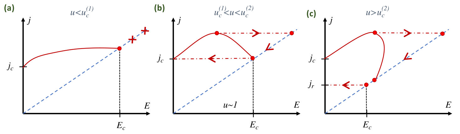 Figure 2
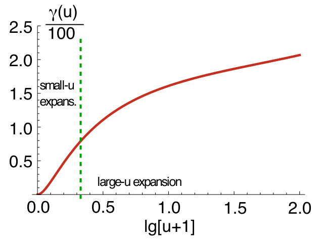 Figure 2
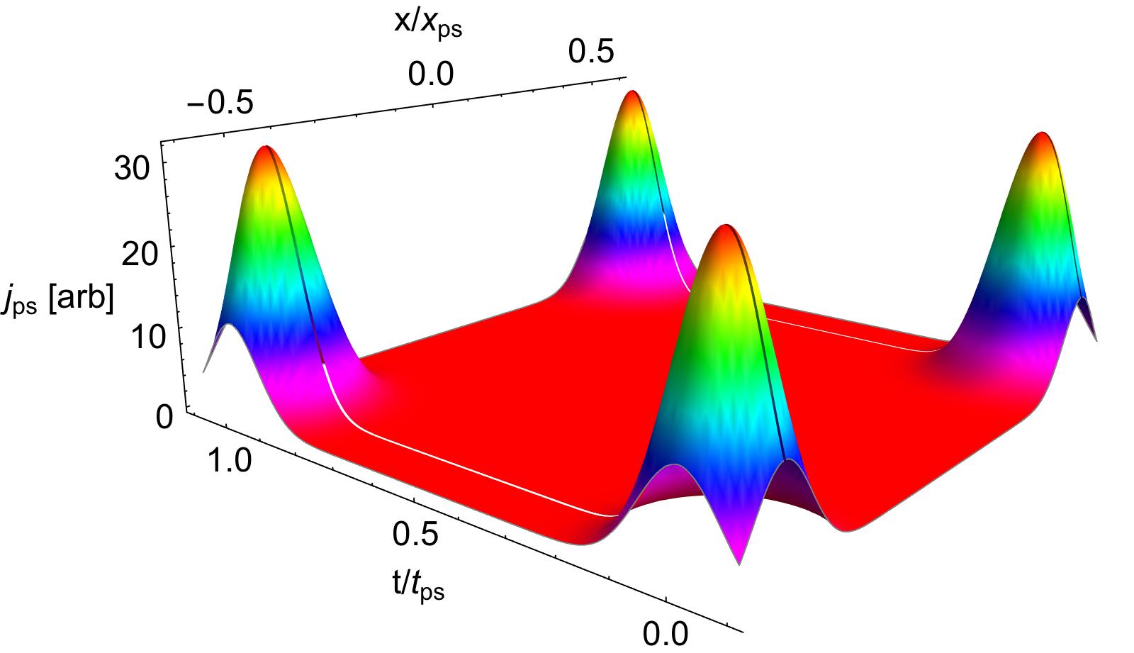 Figure 3
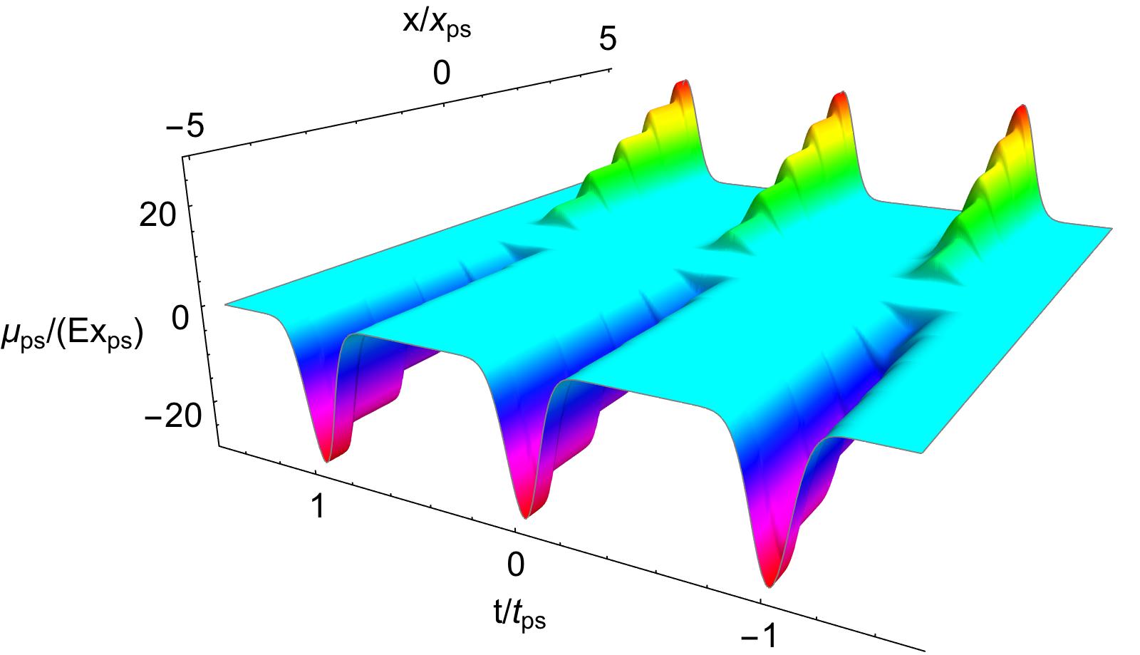 Figure 4
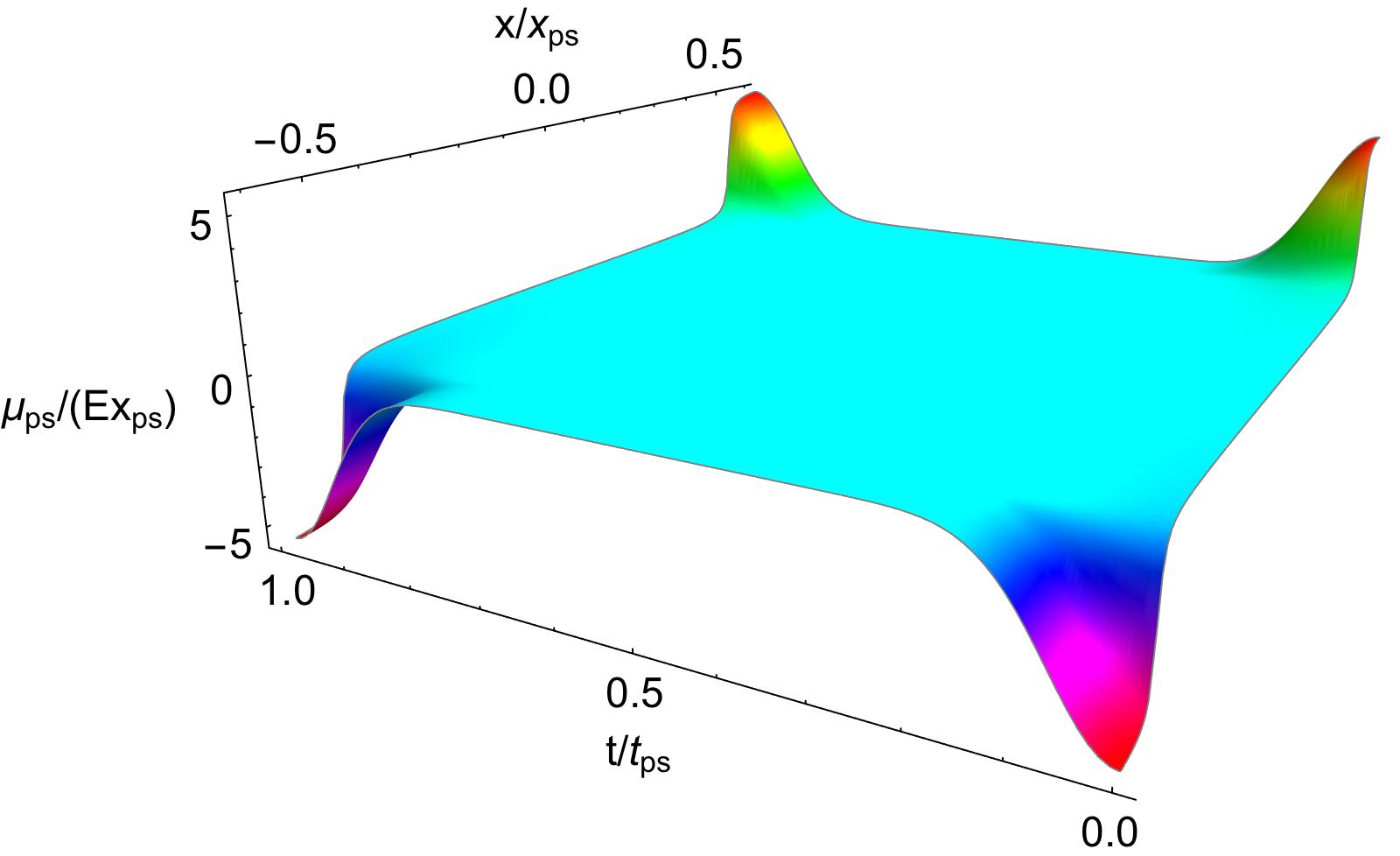 Figure 5
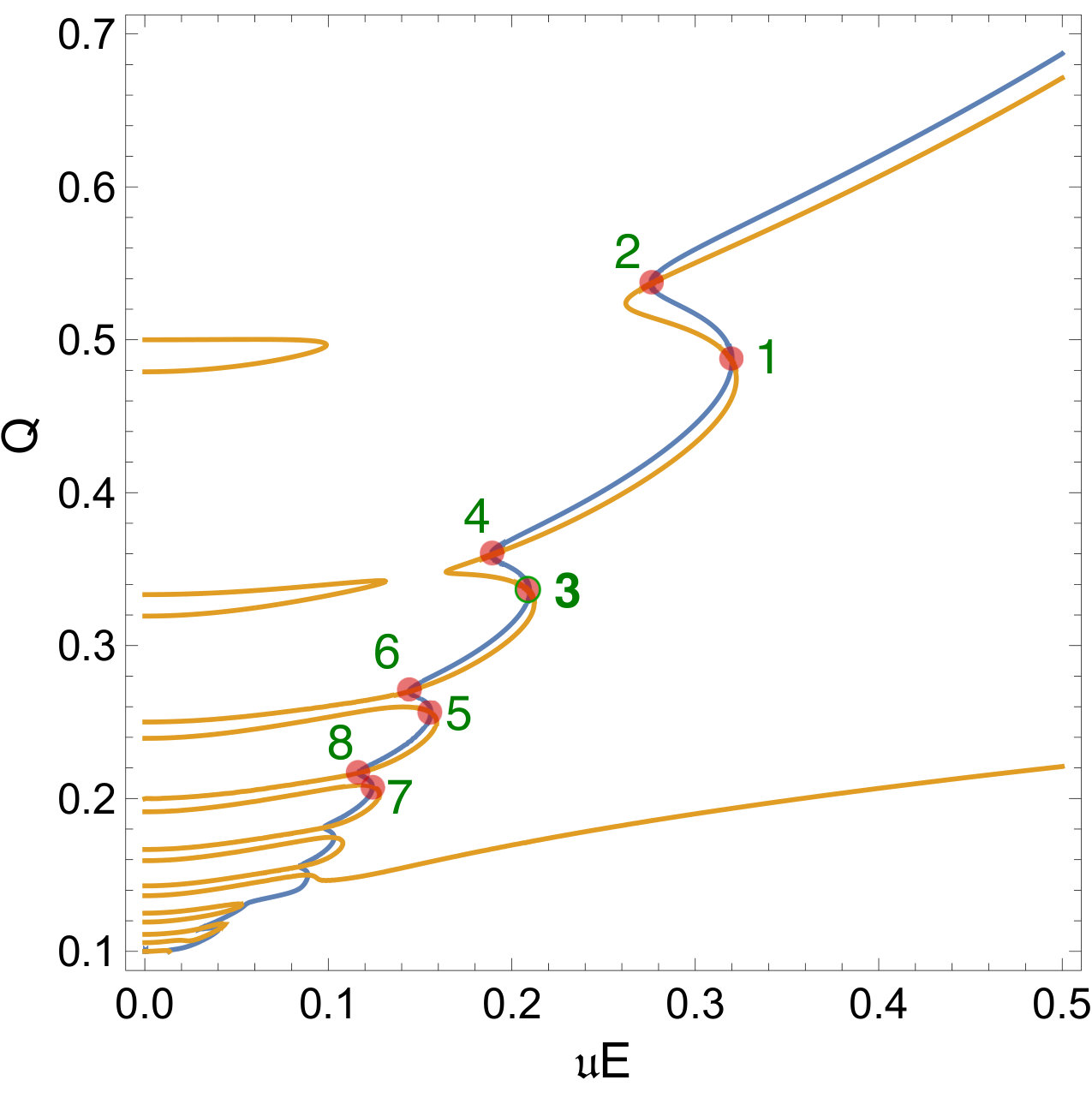 Figure 6
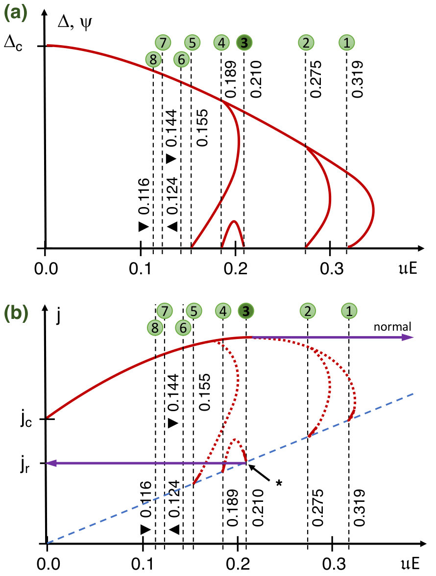 Figure 7
| 1 | 0.320 | 0.486 | 0.166 | -0.503 | -0.176 |
|---|---|---|---|---|---|
| 2 | 0.276 | 0.537 | 0.102 | -0.230 | -0.0787 |
| 3 | 0.21 | 0.335 | -0.0478 | 0.128 | 0.030 |
| 4 | 0.189 | 0.359 | 0.0265 | -0.0671 | -0.0169 |
| 5 | 0.156 | 0.256 | 0.0133 | -0.0345 | -0.00570 |
| 6 | 0.144 | 0.27 | 0.0074 | -0.0183 | -0.00258 |
| 7 | 0.124 | 0.208 | 0.00348 | -0.00922 | -0.000833 |
| 8 | 0.116 | 0.217 | 0.00199 | -0.00528 | -0.000436 |
| 1 | 0.320 | 0.486 | 0.166 | -0.503 | -0.176 | 2.07 |
|---|---|---|---|---|---|---|
| 2 | 0.276 | 0.537 | 0.102 | -0.230 | -0.0787 | 1.97 |
| 3 | 0.21 | 0.335 | -0.0478 | 0.128 | 0.030 | 2.93 |
| 4 | 0.189 | 0.359 | 0.0265 | -0.0671 | -0.0169 | 2.74 |
| 5 | 0.156 | 0.256 | 0.0133 | -0.0345 | -0.00570 | 3.83 |
| 6 | 0.144 | 0.27 | 0.0074 | -0.0183 | -0.00258 | 3.63 |
| 7 | 0.124 | 0.208 | 0.00348 | -0.00922 | -0.000833 | 4.74 |
| 8 | 0.116 | 0.217 | 0.00199 | -0.00528 | -0.000436 | 4.54 |
Peer Reviews
No public reviews on file for this paper yet. If you reviewed it on a platform where reviews are public (OpenReview, ICLR, NeurIPS, ICML), you can paste yours below so the community can read it here.
Videos
No videos yet. Explain this paper in a talk, walkthrough, or lecture? Add one.
Instabilities of the normal state in current-biased narrow superconducting strips
Yury N. Ovchinnikov
Landau Institute for Theoretical Physics, RAS, Chernogolovka, Moscow District, 142432, Russia
Max-Plank Institute for Physics of Complex Systems, 01187 Dresden, Germany
Andrey A. Varlamov
CNR-SPIN (Istituto Superconduttori, Materiali Innovativi e Dispositivi), Viale del Politecnico 1, 00133 Rome, Italy
Gregory J. Kimmel
Materials Science Division, Argonne National Laboratory, 9700 S Cass Avenue, Lemont, IL 60439, USA
Andreas Glatz
Materials Science Division, Argonne National Laboratory, 9700 S Cass Avenue, Lemont, IL 60439, USA
Department of Physics, Northern Illinois University, DeKalb, IL 60115, USA
(March 15, 2024)
Abstract
We study the current-voltage characteristic of narrow superconducting strips in the gapless regime near the critical temperature in the framework of the Ginzburg-Landau model. Our focus is on its instabilities occurring at high current biases. The latter are consequences of dynamical states with periodic phase-slip events in space and time. We analyze their structure and derive the value of the reentrance current at the onset of the instability of the normal state. It is expressed in terms of the kinetic coefficient of the time-dependent Ginzburg-Landau equation and calculated numerically.
reentrance current, phase-slips, critical current, time-dependent Ginzburg-Landau equation
I Introduction
Narrow superconducting strips are the subject of great interest for superconducting quantum electronic devices. Their dissipation-less state is very subtle and sensitive to thermal and quantum fluctuations, which can easily flip the superconducting strip into the resistive state, making them ideal candidates for very sensitive detectors. Various models have been proposed to explain the appearance of non-zero resistance in these strips and its temperature dependence in the region of low temperatures (for a review, see Refs. [Sahu et al., 2009; Bezryadin, 2012]).
The role of thermal fluctuations responsible for energy dissipation, when current flows through a one-dimensional superconductor, was considered for the first time in the seminal paper by Langer and AmbegaokarLanger and Ambegaokar (1967) over fifty years ago. Note, that a realistic “one-dimensional superconductor” is in fact a narrow strip with finite width , much less than the Ginzburg-Landau coherence length , where is the reduced temperature and the critical temperature. The energy dissipation in this system is related to phase-slip processes appearing in thin superconducting wires Tinkham (1996); Skocpol et al. (1974); Kramer and Baratoff (1977); Kramer and Rangel (1984); Rangel and Kramer (1989); Lau et al. (2001); Mooij and Nazarov (2006); McKay et al. (2008); Kimmel et al. (2017) or superfluids Glatz and Nattermann (2002); Scherpelz et al. (2014, 2015), i.e., the processes of vortices/flux quanta crossing the strip.
It is clear, that such events cannot be realized in the framework of a purely one-dimensional model. Indeed, as it was shown in Ref. [Langer and Ambegaokar, 1967], the minimal value of the order parameter magnitude remains finite and equal to even when the density of current flowing through the one-dimensional superconductor reaches the “depairing” value, , and global superconductivity in the one-dimensional channel is only partially suppressed. Yet, the order parameter should become zero at least in one point of the strip in order to allow the system to perform a phase slip event. 111Note, that, in contrast to the one-dimensional superconducting strip, the order parameter in a higher-dimensional superconductor becomes zero when the current density approaches the “depairing” value.
The apparent paradox occurring in the one-dimensional case was resolved in Ref. [Ovchinnikov and Varlamov, 2015]. The authors demonstrated that the saddle point solutions of the static Ginzburg-Landau (GL) equations for the order parameter in the presence of a fixed current density , possessing at least one vortex, exist only for very weak current densities . In the case , such phase-slip events are possible, which are random in space and time due to thermal fluctuations. When the current density exceeds the value , the static scenario described above does not hold anymore. In this region () dynamical states are formed in the strip, where phase-slip events occur periodically in space and time 222Note that material defects and weak links also lead to phase-slip events Kramer and Watts-Tobin (1978); Watts-Tobin et al. (1981); Berdiyorov et al. (2014); Kimmel et al. (2017), but here we concentrate on the clean case..
In this paper we study the hysteretic structure of such dynamical states of a narrow superconducting strip and obtain the corresponding current-voltage (–) characteristics. In particular, we derive the value of the re-entrance current density , at the onset of the instability of the normal state, when the applied current decreases. Our consideration is valid in the gapless region, at temperatures slightly below the critical one, where the time-dependent Ginzburg-Landau equation holds. In this situation, we investigate the strong current regime of the superconducting strip being in its dynamical state up to second order perturbation theory in the electric field .
It is important to note, that the considered situation is quite different from the problem of determining the critical current at which the superconductor becomes normal (see Refs. [Ivlev and Kopnin, 1984; Kopnin and Ivlev, 1984]). The authors of the cited papers, which are based on the works by Gorkov Gorkov (1970) and Kulik Kulik (1971), claim that the normal state remains stable for any finite value of . However, they ignore the fact that the exponential growth of superconducting fluctuations in a time interval determined by leads to an instability of the normal state ( is the normal conductivity). As a result, the system enters a dynamical superconducting state at some finite electric field. We will show below that there are many values of the parameter for which the normal state starts to be unstable even for infinitely small perturbations.
In the following we describe the model and show the analysis of the time-dependent Ginzburg-Landau equation near the critical point of the normal state. We derive the value of the reentrance current and order parameter values using first order perturbation theory by small deviation from the critical point. Details of the calculations can be found in the Appendices. We start with introducing the model in the following section and then analyze the –characteristics close to the deparing current and near the instability points of the normal state.
II Model
In this paper we approximate the narrow superconducting strip of width smaller than the superconducting coherence length by a one-dimensional (1D) system, described by the time-dependent Ginzburg-Landau equation (TDGLE). The TDGLE can be written in dimensionless variables, without accounting for thermal fluctuations and magnetic field (the latter does not appear in the 1D model) in the form
[TABLE]
where is the complex order parameter and is the scalar potential. The reduced relaxation rate controls the system’s evolution in time and is given by
[TABLE]
where is the density of states at the Fermi surface, is the effective diffusion constant, is the Riemann-Zeta function, and is a numerical constant.Ovchinnikov (1997); Kopnin (2001)
The fixed total bias-current consists of the sum of normal () and superconducting () components and in its turn can be related to the space derivatives of the complex order parameter and the scalar potential:
[TABLE]
Time and distance in Eqs. (1)-(3) are measured in units of and scaled superconducting coherence length, , respectively, with being the London penetration depth. The electrical current density is measured in units of ( is the flux quantum). In these units the depairing current density reads as .
In what follows, it is useful to transform the scalar potential to the form
[TABLE]
where is the average electric field, which is equal to the average normal current in dimensionless units, and is the spatially and temporally fluctuating part of .
Phase-slip events generate instabilities in the current-voltage characteristics, which will be the main subject of this work. In particular, these processes cause strong changes in the electric field and order parameter at their space-time coordinates. We take their effect into account explicitly by introducing a corresponding effective electric potential to the TDGLE.
A phase-slip process in a strip of finite width is related to the transfer of a magnetic vortex-antivortex pair across it. Each such event is accompanied by the suppression of the order parameter and, consequently, of the supercurrent. Due to the conservation of the total current, a sharp peak in the normal current appears at the time and space location of the phase-slip event.
In the large-current regime, , these phase-slip events (ps) are periodic in time and space. The corresponding periods in time and space are denoted as and , respectively. Outside a very narrow region in the time-space plane one can rewrite Eq. (1) in the form
[TABLE]
Here and the associated potential
[TABLE]
where the quantization condition is implied. The shape of is illustrated in Fig. 1 (top) with smoothed step and delta functions. In the bottom panels and are shown in the elementary space-time cell . The latter illustrating the mentioned spikes in the normal current at the phase slip event location.
These additional terms do not contribute to the electric field inside but only at its corners. The solution for the order parameter away from the corners of follows from Eq. (5) with periodic boundary conditions. The size of the region with strong suppression of is of order , where is the width of the strip.
III Analysis of the –characteristics
Let us start with the analysis of Eqs. (1)-(4). Within the unit cell , one can make the Fourier-Ansatz for the complex order parameter
[TABLE]
where should be found from local minimum conditions of for a given current density .
Correspondingly, Eq. (3) acquires the form
[TABLE]
Plugging Ansatz (7) into Eq. (1) gives
[TABLE]
Finally, accounting for the charge conservation condition and Eq. (3), one can find the expression for the fluctuating part of the scalar potential in terms of the introduced Fourier coefficients:
[TABLE]
In Eqs. (9)-(10) we explicitly separated the quantity , since it is the dominant Fourier component in the vicinity of the critical point and plays an important role throughout the paper. Fourier coefficients with quickly decay. All other coefficients in this region can be found in the framework of perturbation theory.
Eq. (9) enables us to obtain the –characteristics in the complete domain of dynamical resistive states. The above mentioned minimization with respect to allows us to finds the shape of the –characteristics, which turns out to be critically dependent on the value of the dynamic coefficient of the TDGLE.
One can expect to find three qualitatively different types of –characteristics, which are illustrated in Fig. 2. The first one (Fig. 2a) is reversible and could be realized when the dynamic coefficient is sufficiently small: , where is the first critical value, which will be obtained below. In case the –characteristics becomes irreversible (Fig. 2b,c).
In the case of strong damping, when exceeds the second critical value , the transition to a finite value of the order parameter happens at a smaller value, which is where we define the reentrance current . Calculation of the order parameter value in the vicinity of the critical point (see below) shows that in practice only the latter scenario of the –characteristics, shown in Fig. 2c), is realized.
III.1 Current density close to the depairing current
Next, we consider the case when the bias current density is close to . Eq. (1) allows us to obtain the above mentioned value of , which destroys superconductivity in the 1D channel, where the corresponding critical value of the order parameter is , and the value of wave-vector (for ) . Close to this point, Eq. (9) is decomposed into two equations with . A detailed analysis of the Fourier coefficients and the determination of the wave vector is presented in Appendix A. As a result of these calculations we obtain the electric field dependence of the current density to second order, close to its depairing value as
[TABLE]
where the calculation of the coefficient of the quadratic term as function of is a highly involved task, but can be performed exactly for any value of and be expressed as a full derivative:
[TABLE]
The explicit expression of the full derivative is given in Appendix A, Eq. (33), and is defined there in Eqs. (26b) and (27). Note, that the difference in braces behaves as for small , such that all terms under the derivative cancel and the complete expression is non-singular at . Therefore, in the limit of small we keep the first two terms of the sum in (12) and expand the remaining sum to first order. This gives
[TABLE]
For large values of (), we obtain from Eq. (12) (using the asymptotic expressions of the and terms)
[TABLE]
The -dependence of and the domains of validity of its approximations (13)-(14) are presented in Fig. 3. separates the regions where small- and large- approximations work best, i.e., the relative deviations from the exact curve are both minimum at , less than .
III.2 Vicinity of the critical points
We now consider the vicinity of critical points, , which are defined by the condition
[TABLE]
In this region we search for the solution to the non-linear problem (9) by its linear expansion over eigenfunctions. Therefore the linearized condition of Eq. (15) can be understood as the following eigenvalue problem
[TABLE]
where the form of the linear operator follows from Eq. (9):
[TABLE]
with
[TABLE]
The eigenvector of Eq. (16) is related to the Fourier coefficients at the critical points in the following way
[TABLE]
where .
The above eigenvalue problem has possibly an infinite number of solutions . Note, that the quantities and only appear in the form of a product at the critical point [in contrast to Eqs. (11) & (12)]. The linearized equation can be solved numerically and the largest eight critical points (defined by simultaneous eigenvalues of and ) are listed in table 1 [the corresponding normalized eigenvectors of and (here ) are given in the supplementary information]. Below we discuss the numerical solution in more detail.
In order to get further insight into the behavior of the –characteristic near these critical points and to determine the type of instability point (first or second order transition), we introduce the operator as
[TABLE]
with
[TABLE]
[compare to Eq. (18)].
Near a critical point the solution for the Fourier components in Eq. (9) in our linearized approximation can be written in the form
[TABLE]
with the proper permutation of -indices as defined in Eq. (19) and where the coefficient follows from the solvability condition
[TABLE]
see Appendix B for explicit expressions for all coefficients .
The expression for current density then takes the form
[TABLE]
(see Appendix B for definition of .)
We note, that in the critical region only the coefficient of the zero mode, , is dominant and all other coefficients are small, scaling with .
Altogether, we can now analyze the critical point in detail. Therefore we calculate the critical points numerically for truncated Fourier series with components (indices ). These are obtained as simultaneous solutions of the polynomial equations and of order in . Figure 4 shows the solutions for (order ), where the solid lines represent the solutions of the individual equations. Note, that solving the linearized equations for the truncated Fourier series leaves the largest critical values invariant for sufficiently large . For these solutions we can then obtain the eigenvectors of and , which allows us then to extract the behavior of the –characteristic near these critical points by evaluation of the parameters , , and . At those points new branches appear, which can bring the system out of the normal state. Using Eq. (23b) then defines the slope of the linearized –characteristic. The numerical calculation reveals that the critical value , , has locally a negative slope among the eight largest values, indicating that a reentrance into the superconducting state can happen without a threshold (second order) at a current density . Fig. 5 shows the behavior of the order parameter , (a), and current , (b), at the critical points as a function of . The connection of the critical points to the envelop (defined by the –curve for increasing current) is indicated by dotted lines (these cannot be realized physically). Practically, one can make a ‘hysteresis ‘loop” in the - diagram by starting in the superconducting state at zero current, following up to upon increasing , where the system becomes resistive and eventually jumps into to normal state (indicated by an arrow) following the normal –curve (blue, dashed). When decreasing from the normal state, one follows down the normal –-line till the critical point labeled (), where the slope of –is negative, such that fluctuating superconducting regions can grow and one jumps back into the superconducting state at (indicated by an arrow). Below this point the normal state is always unstable. At all other (larger) critical points we cannot follow the critical –(without threshold) as the slope is positive (first order). We note that the specific picture depends on the actual value of for the physical system under consideration, here we assume a value of of order one.
The numerical analysis demonstrates that probably an infinite set of solutions of the eigenvalue problem, Eq. (16) exists.
In analogy to finding the (global) extremum of a function on a finite support, where also the boundary values need to be checked, here we should also study the properties of the system close to the hypothetical “endpoints”, if those exist [besides the (local) critical points defined by (16)]. By “endpoints” we mean points of the surface in Hilbert space, where the value reaches its maxima under the condition
[TABLE]
Our numerical evaluation of this condition reveal that such “endpoints” are irrelevant.
IV Conclusions
We have investigated the –characteristic of a superconducting strip in the region near the depairing current and studied the instability points of the normal state as function of the current. Interestingly, one finds a degeneracy in second order perturbation theory in the electric field by solving linearized equation at those critical points.
This degeneracy leads to the appearance of additional branches splitting off from the Ohmic behavior seen in Fig. 5. Numerically, we calculated the critical points and found that the largest electric field value, at which the normal state first becomes unstable upon decreasing the current, i.e., indicating the possibility of a transition into the superconducting state with finite value of the order parameter amplitude (see Fig. 5a), and a branch in the –appears is at . However, the slope of the branch is positive, indicating a first order transition, which we can only follow when increasing the current (and eventually jumping back in the normal state). Therefore, when increasing the current for fixed in the intervals or , a transition into the superconducting state will happen at or , respectively, before returning to the normal state at larger currents.
However, most importantly, we also found the smallest value for when the normal state is always unstable to be equal to (indicated by in Fig. 5), defining the reentrance current into the superconducting state. In contrast to the evaluation of the critical current, the evaluation of the re-entrance current is significantly more involved.
Acknowledgments
We are delighted to thank I.S. Aranson for interesting discussions. The research was supported by the U.S. Department of Energy, Office of Science, Basic Energy Sciences, Materials Sciences and Engineering Division.
Yu.N.O acknowledges Prof. Dr. Jeroen van den Brink for his hospitality in LIFW and the DFG for granting him a Mercator-Professoren-Stipendium. A. V. acknowledges financial support from the project CoExAn (HORIZON 2020, grant agreement 644076), from Italian MIUR through the PRIN 2015 program (Contract No. 2015C5SEJJ001).
Appendix A Solution of TDGLE near the depairing current
Close to the depairing current, Eq. (9) is decomposed into pairwise equations with .
For 1
[TABLE]
Solving this system results in
[TABLE]
In our approximation, we obtain from Eq. (26b)
[TABLE]
when the electric field is much smaller than its critical value .
For , we obtain from Eq. (9), the following equation for the quantity in second order perturbation theory
[TABLE]
Using second order perturbation theory, we can set
[TABLE]
where are constants. Inserting expression (26a) for the coefficients and expressions (29) into Eq. (28), we get the following relation for those constants:
[TABLE]
One important property of Eqs. (28) and (29) should be mentioned: in second order perturbation theory, defined by Eq. (30), and appear only in combination . This implies that corrections to the quantities and appear separately in perturbation theory only in order
In the same approximation we obtain from Eq. (8)
[TABLE]
Inserting Eq. (30) into expression (31) yields an expression for the current in second order perturbation theory in :
[TABLE]
The expression for in (32b) can be evaluated explicitly as
[TABLE]
which can be written as the full derivative Eq. (12).
Appendix B Solvability and –at the critical points
The coefficients in the solvability equations, (23a) and (23b), are given by
[TABLE]
Here are the components of the normalized eigenvector of the transposed operator .
Next, we define the function
[TABLE]
where are the components of the eigenvector of and are the components of the normalized eigenvector of the operator . Function is defined in Eq. (20). Eq. (9) in the vicinity of each critical point can then be rewritten in the form
[TABLE]
where the coefficients are given in (34a)-(34c). Therefore:
[TABLE]
The functions corresponding to the eight largest critical value are given by
[TABLE]
Note the signs of the coefficients in . For completeness, we reproduce the corresponding eigenvectors and in the supplementary information.
Appendix C Derivation of Fourier equations
Here we will obtain the equation system for the Fourier coefficients . From Eq. (9) we obtain for
[TABLE]
From Eq. (9) we obtain a separate equation for :
[TABLE]
Next, we introduce the operator for as
[TABLE]
With this, Eq. (1) can be written in the form
[TABLE]
where is
[TABLE]
Note, that a free parameter appears in Eqs. (37) and (39). The value of this parameter is found by the extremal condition for the electric field for a given current density .
Appendix D Supplementary Information: Eigenvectors near critical points
Here we present detailed results of the numerical evaluation at critical points including the eigenvectors. All calculations are done for (Fourier) components of the eigenvectors of and , and , respectively. Here component indices range from .
The results for the eight largest critical are reproduced in table 2, including the critical structural constant , and the four parameters (); see manuscript. The bold printed critical value 3 corresponds to the reentrance point.
The normalize eigenvectors and functions (see manuscript) are listed below, where bracketed superscripts correspond to the index in table 2. The component is printed in bold.
[TABLE]
[TABLE]
Note, the eigenvectors are only defined up to an overall factor.
The reference list from the paper itself. Each links out to its DOI / PubMed record.
- 1Sahu et al. (2009) M. Sahu, M.-H. Bae, A. Rogachev, D. Pekker, T.-C. Wei, N. Shah, P. M. Goldbart, and A. Bezryadin, Nature Physics 5 , 503 (2009) . · doi ↗
- 2Bezryadin (2012) A. Bezryadin, Superconductivity in Nanowires: Fabrication and Quantum Transport , 1st ed. (Wiley-VCH, 2012).
- 3Langer and Ambegaokar (1967) J. S. Langer and V. Ambegaokar, Phys. Rev. 164 , 498 (1967) . · doi ↗
- 4Tinkham (1996) M. Tinkham, Introduction to superconductivity (Courier Corporation, 1996).
- 5Skocpol et al. (1974) W. J. Skocpol, M. R. Beasley, and M. Tinkham, J. Low. Temp. Phys. 16 , 145 (1974) . · doi ↗
- 6Kramer and Baratoff (1977) L. Kramer and A. Baratoff, Phys. Rev. Lett. 38 , 518 (1977) . · doi ↗
- 7Kramer and Rangel (1984) L. Kramer and R. Rangel, J. Low. Temp. Phys. 57 , 391 (1984).
- 8Rangel and Kramer (1989) R. Rangel and L. Kramer, J. Low. Temp. Phys. 74 , 163 (1989).