Boundary Tensor Renormalization Group
Shumpei Iino, Satoshi Morita, Naoki Kawashima

TL;DR
This paper introduces a boundary tensor renormalization group algorithm that enables the study of both bulk and boundary properties in statistical systems, revealing boundary fixed points and conformal structures at criticality.
Contribution
It extends the tensor renormalization group method to include open boundaries, capturing boundary phenomena and conformal boundary conditions.
Findings
Boundary tensors exhibit fixed point structures similar to bulk tensors.
At criticality, boundary fixed point tensors encode conformal tower information.
The method allows analysis of surface magnetization and boundary critical phenomena.
Abstract
We develop the tensor renormalization group (TRG) algorithm for statistical systems with open boundaries, which allows us to investigate not only the bulk but also the boundary property, such as the surface magnetization. We demonstrate that the tensors representing the boundary in our algorithm exhibit the fixed point structures just as bulk tensors in previous TRG algorithms. At criticality, the scale-invariant boundary fixed point tensors have the information of the conformal tower, which is described by the underlying boundary conformal field theory.
Click any figure to enlarge with its caption.
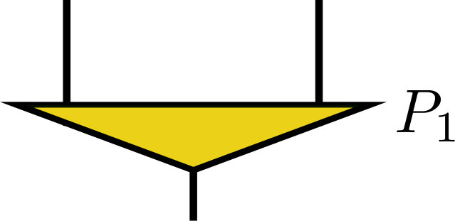 Figure 1
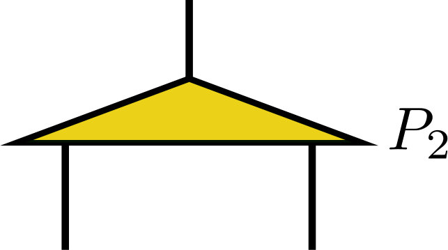 Figure 2
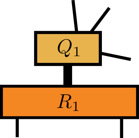 Figure 3
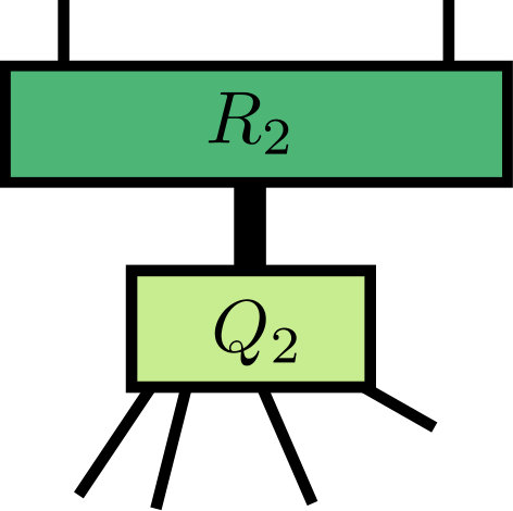 Figure 4
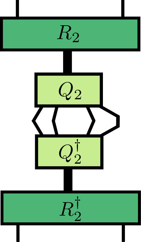 Figure 5
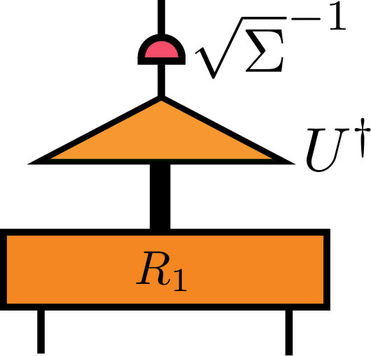 Figure 6
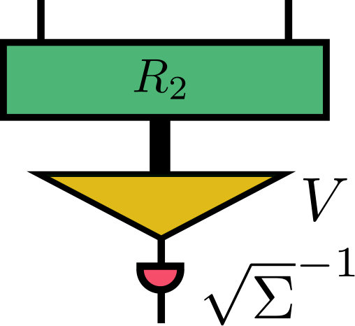 Figure 7
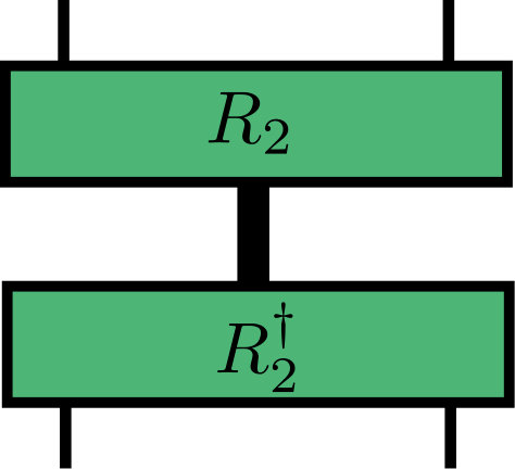 Figure 8
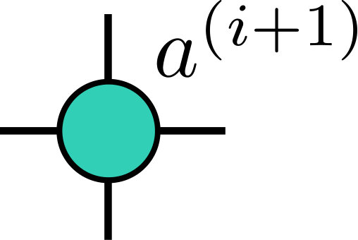 Figure 9
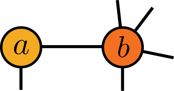 Figure 10
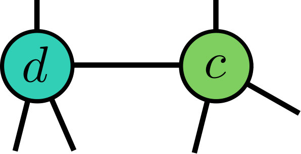 Figure 11
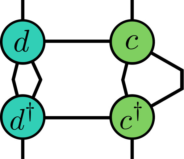 Figure 12
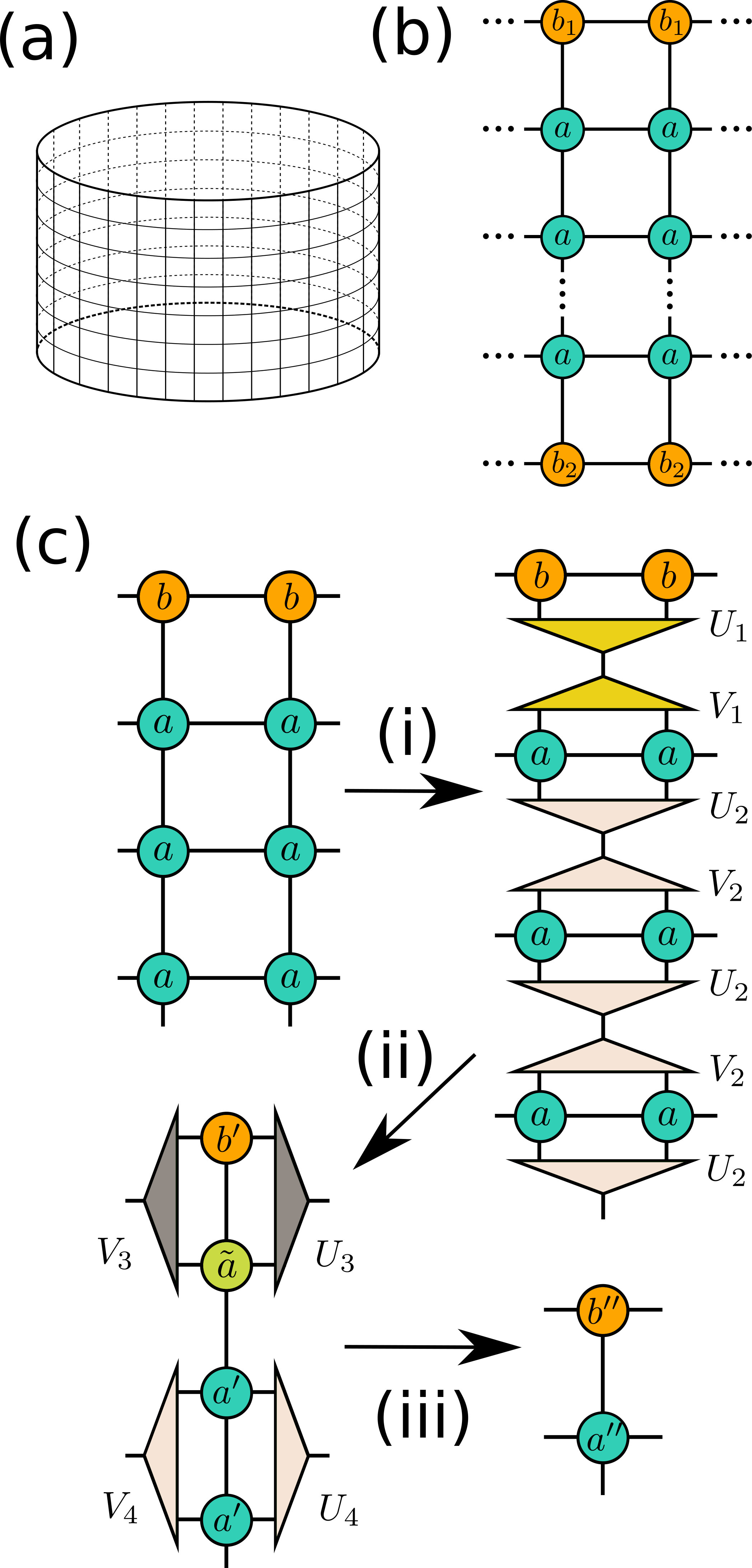 Figure 13
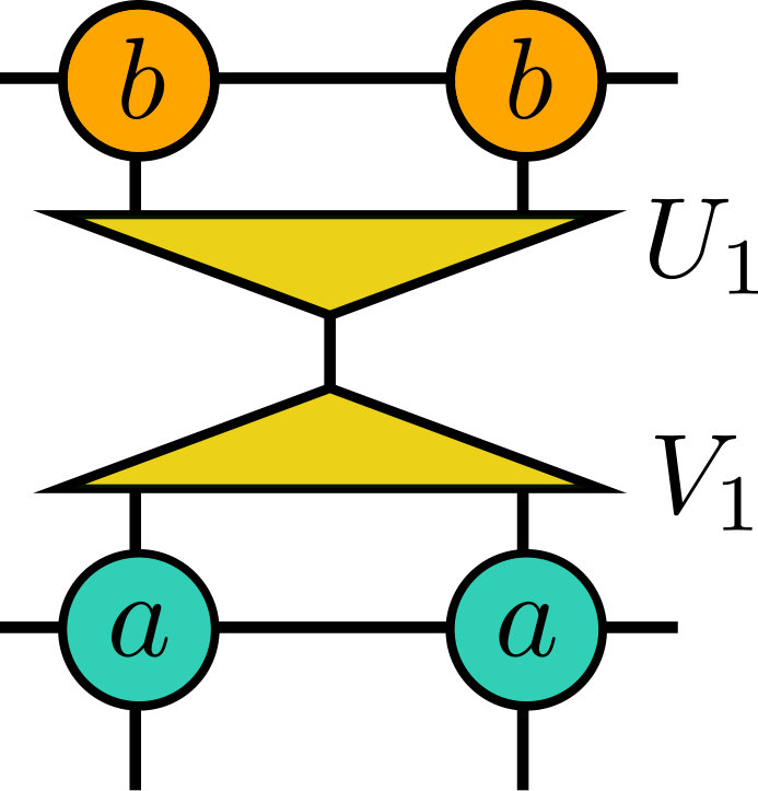 Figure 14
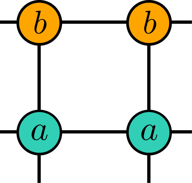 Figure 15
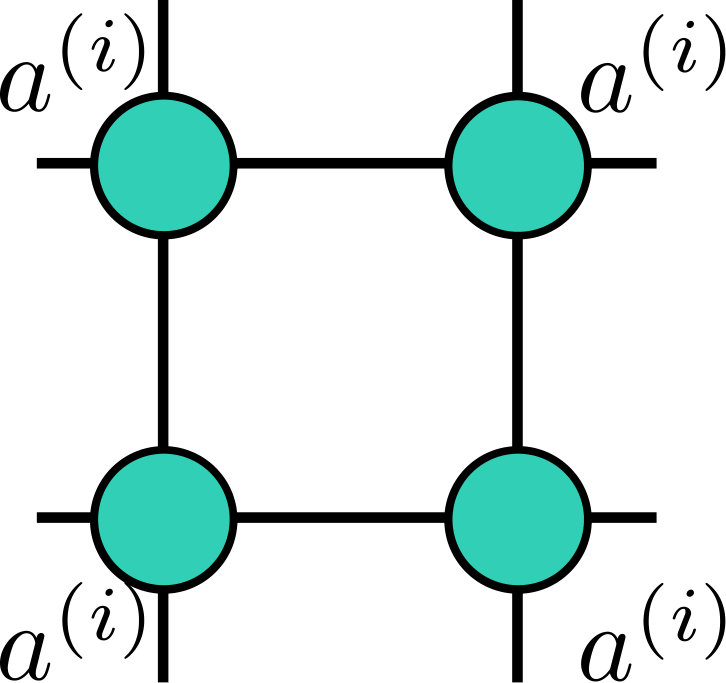 Figure 16
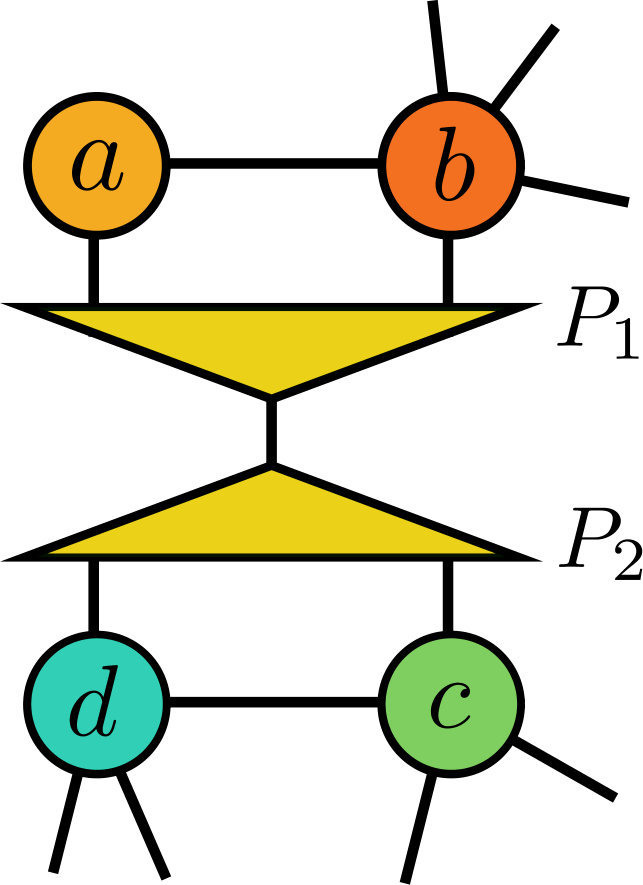 Figure 17
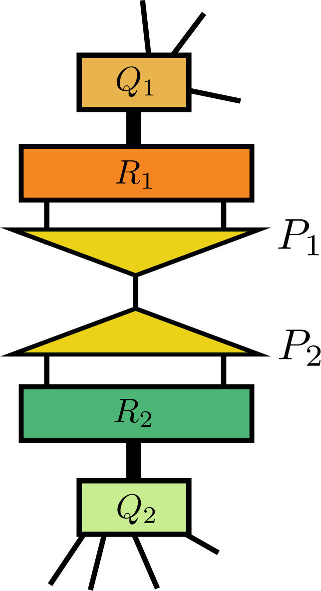 Figure 18
 Figure 19
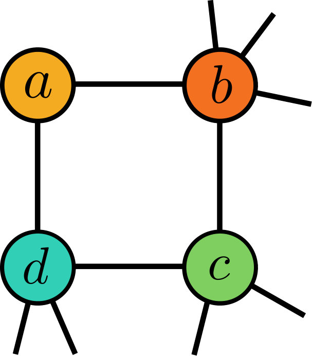 Figure 20
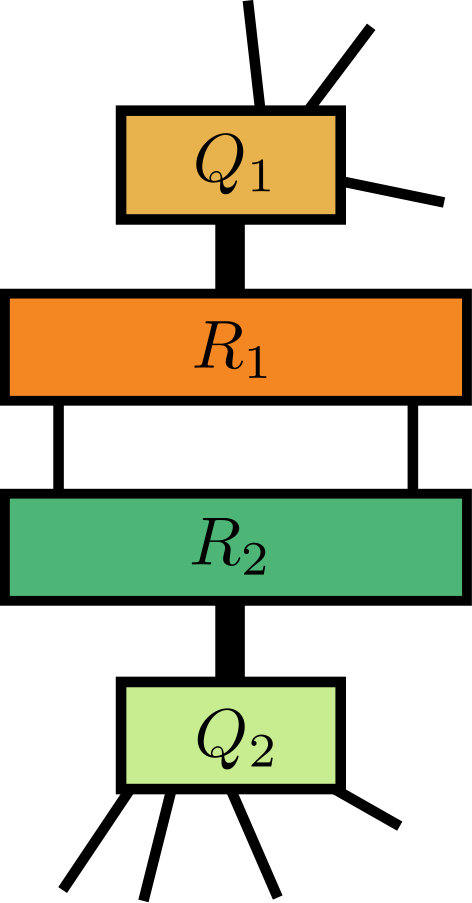 Figure 21
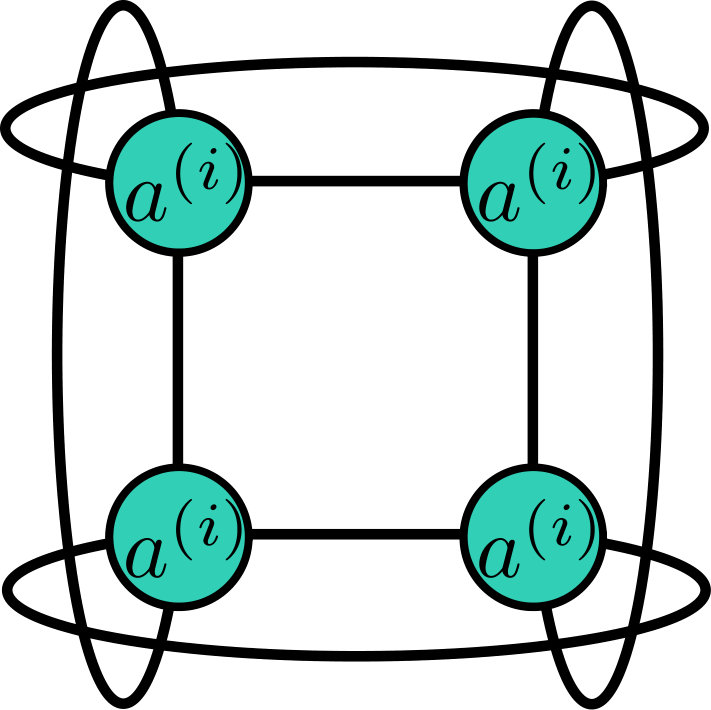 Figure 22
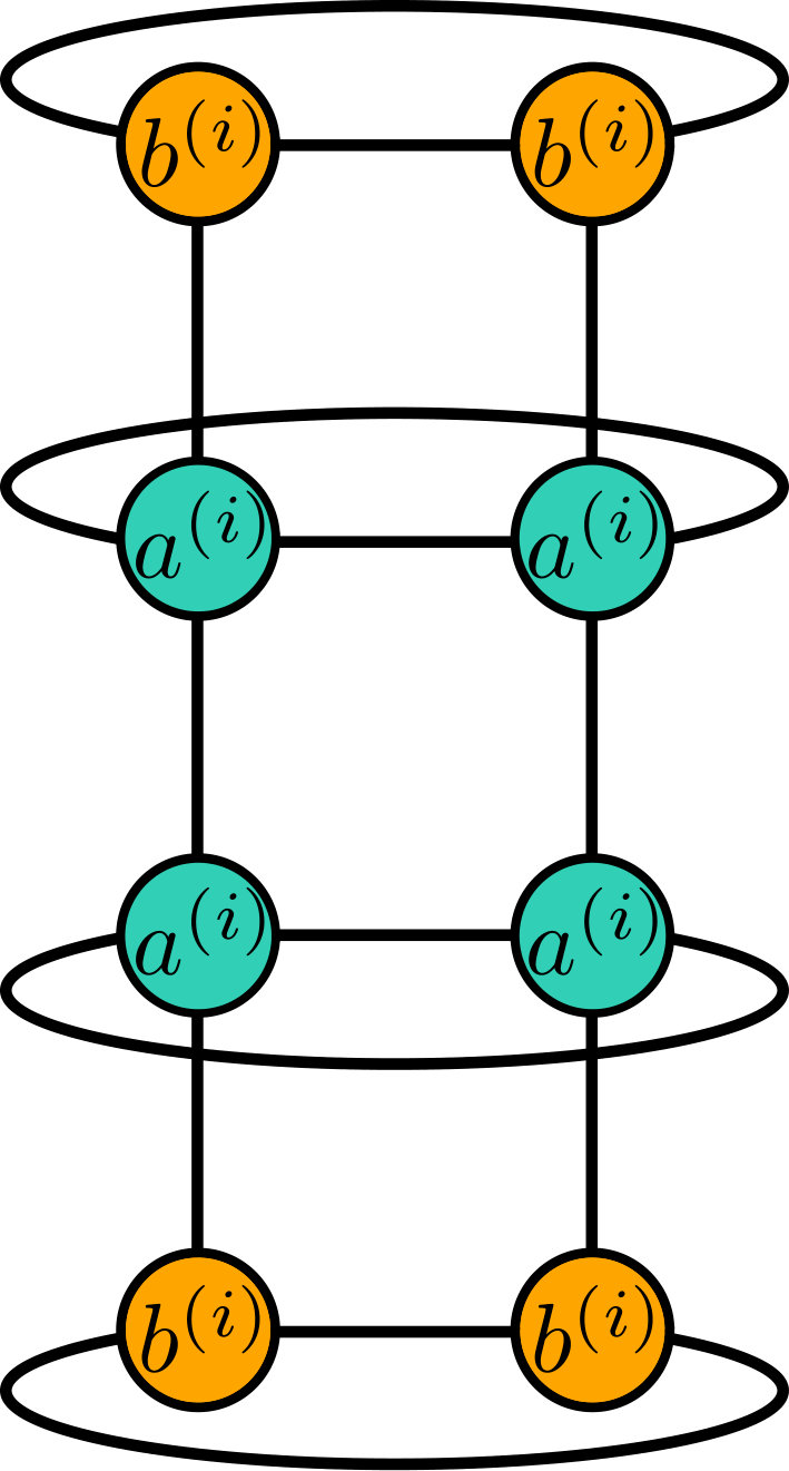 Figure 23
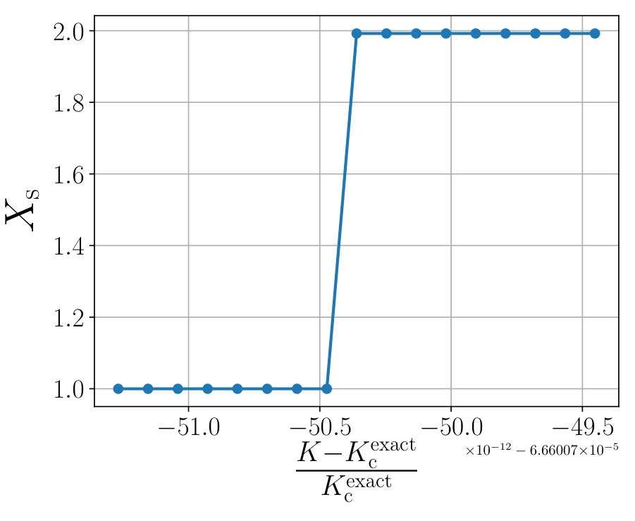 Figure 24
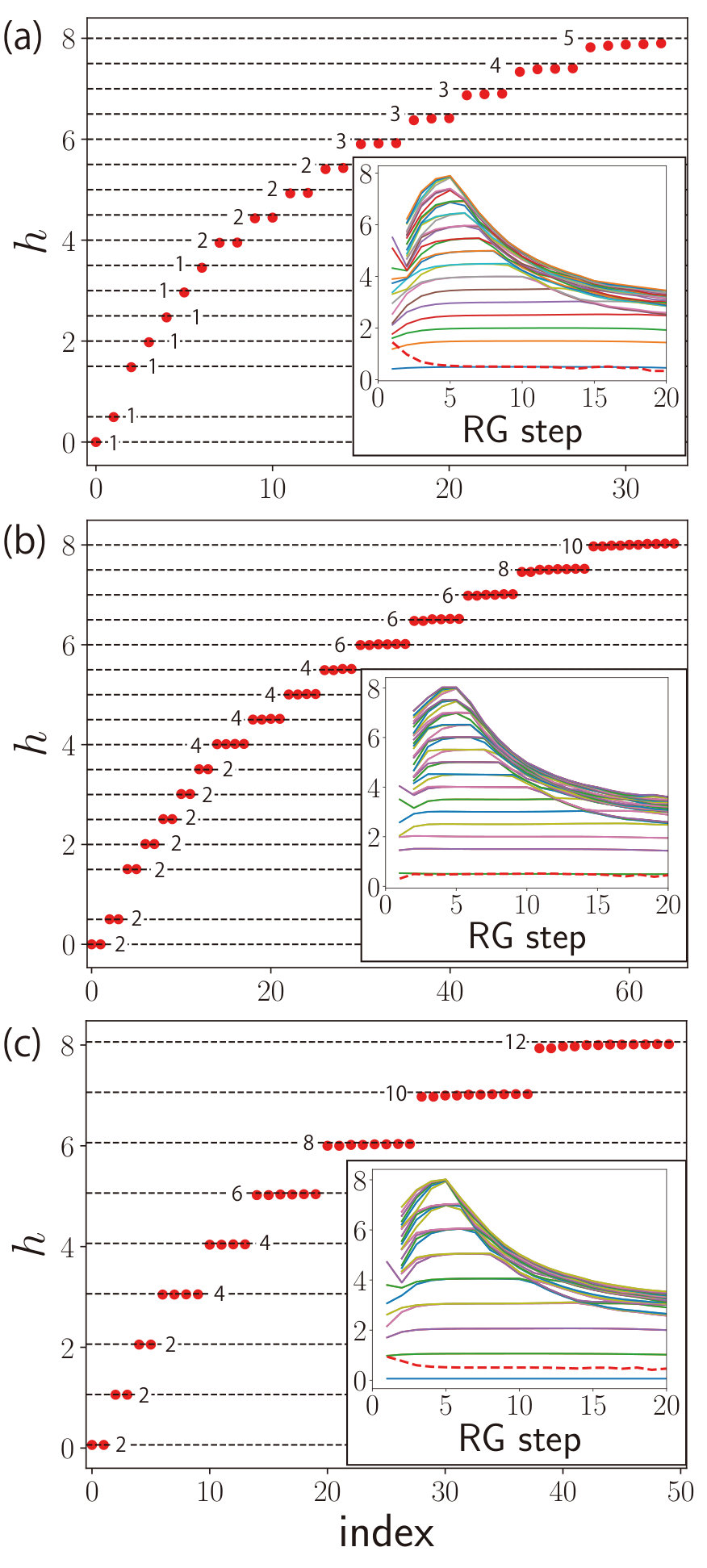 Figure 25
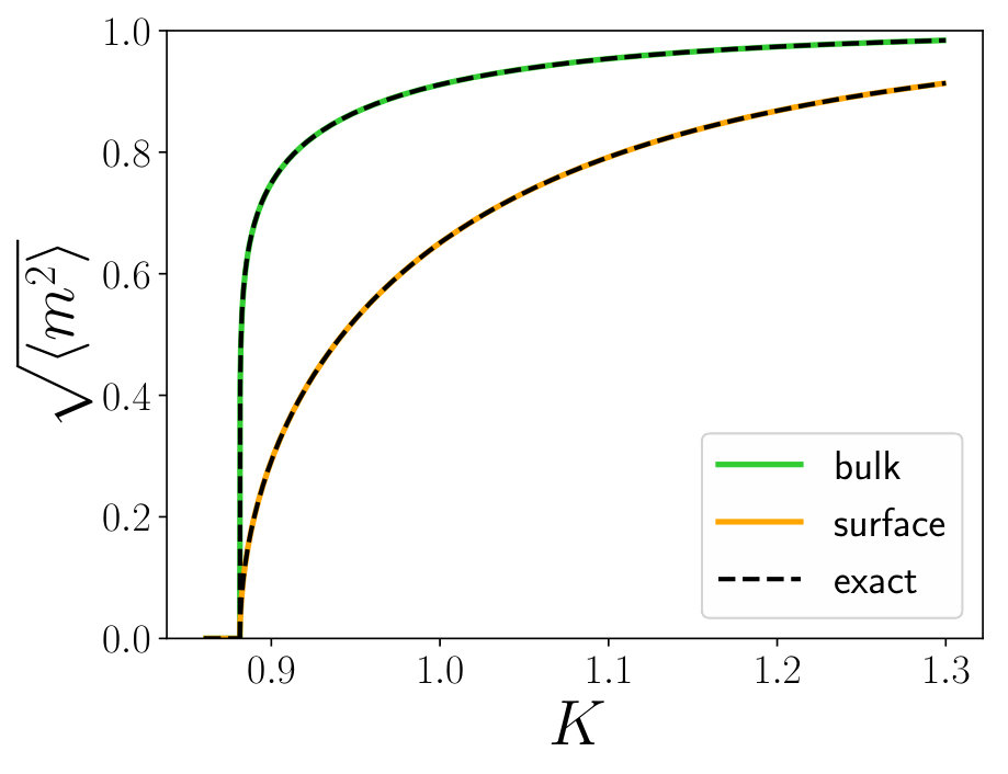 Figure 26
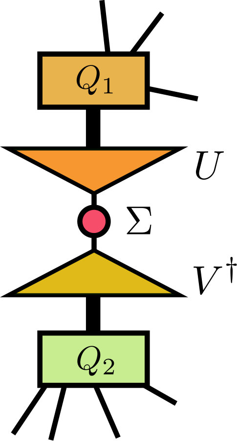 Figure 27
 Figure 28
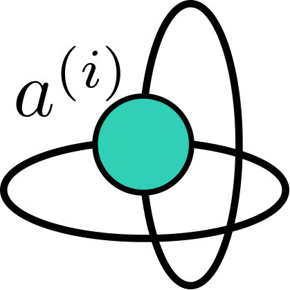 Figure 29
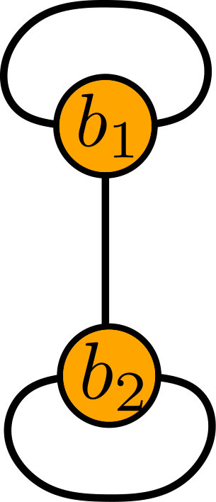 Figure 30
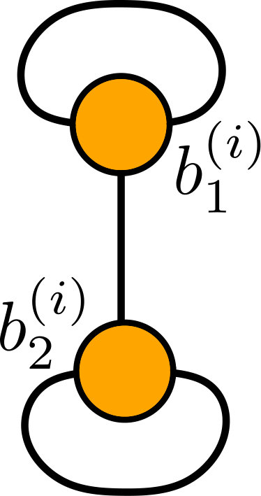 Figure 31
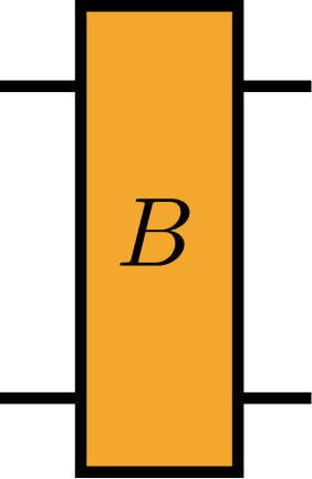 Figure 32
 Figure 33
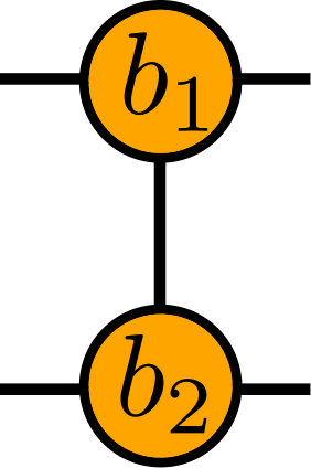 Figure 34
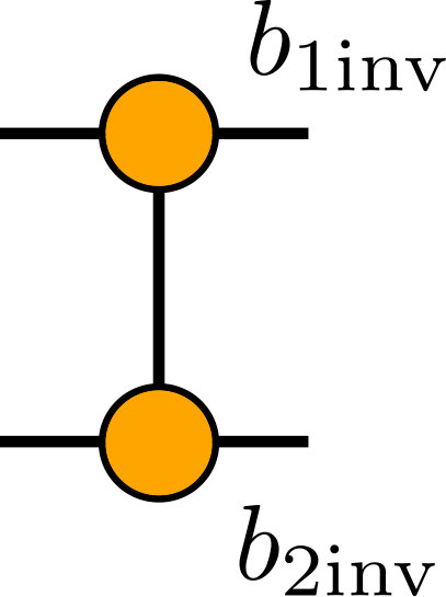 Figure 35
| RG step | 1 | 2 | 3 | 4 | 5 | 6 | 7 | 8 | 9 | 10 | 11 | 12 |
|---|---|---|---|---|---|---|---|---|---|---|---|---|
| boundary | 1.4513 | 0.9776 | 0.6920 | 0.5864 | 0.5411 | 0.5208 | 0.5123 | 0.5101 | 0.5086 | 0.5032 | 0.4954 | 0.4889 |
| bulk | 0.5641 | 0.5188 | 0.5038 | 0.5009 | 0.5002 | 0.4999 | 0.4994 | 0.4984 | 0.4970 | 0.4948 | 0.4920 | 0.4877 |
Peer Reviews
No public reviews on file for this paper yet. If you reviewed it on a platform where reviews are public (OpenReview, ICLR, NeurIPS, ICML), you can paste yours below so the community can read it here.
Videos
No videos yet. Explain this paper in a talk, walkthrough, or lecture? Add one.
Boundary Tensor Renormalization Group
Shumpei Iino
Institute for Solid State Physics, The University of Tokyo, Kashiwa, Chiba, Japan
Satoshi Morita
Institute for Solid State Physics, The University of Tokyo, Kashiwa, Chiba, Japan
Naoki Kawashima
Institute for Solid State Physics, The University of Tokyo, Kashiwa, Chiba, Japan
Abstract
We develop the tensor renormalization group (TRG) algorithm for statistical systems with open boundaries, which allows us to investigate not only the bulk but also the boundary property, such as the surface magnetization. We demonstrate that the tensors representing the boundary in our algorithm exhibit the fixed point structures just as bulk tensors in previous TRG algorithms. At criticality, the scale-invariant boundary fixed point tensors have the information of the conformal tower, which is described by the underlying boundary conformal field theory.
I Introduction
Renormalization group (RG) is one of the most significant concepts in modern physics Wilson (1971a, b). Apart from its original motivation, the prescription for the divergent physical quantity in the quantum field theory, the RG method has been useful to classify the phases, investigate the critical phenomena, and so on Cardy (1996). The philosophy of RG has also been adopted to invent efficient numerical methods, such as density matrix renormalization group (DMRG) White (1992, 1993), corner transfer matrix renormalization group (CTMRG) Nishino and Okunishi (1996, 1997), and entanglement renormalization Vidal (2007). Recent interpretation of RG, ‘efficient compression of information’ draws attention in the field of information science Evenbly and White (2016), especially machine learning Mehta and Schwab (2014).
Combining the real-space RG concept with tensor network representation of the partition function, Levin and Nave proposed tensor renormalization group (TRG) algorithm to contract the tensor network of the Boltzmann weight for statistical systems Levin and Nave (2007). In addition to the capability to compute free energy with high accuracy, as they pointed out, the renormalized tensors show fixed point structures characterizing the corresponding phases. Gu and Wen investigated the precise meaning of this statement, and clarified that it consists of trivial tensors Gu and Wen (2009). Further interestingly, the fixed point tensor at a critical point becomes scale invariant, from which one can extract the information of the underlying conformal field theory (CFT).
‘Boundary’ is another significant keyword in modern physics. The remarkable feature of topological insulators is the metallic surface state even though the bulk is insulator, and Majorana fermions emerge at the edge of topological superconductors Hasan and Kane (2010); Qi and Zhang (2011). The symmetry protected topological (SPT) phases have the gapless or degenerated nontrivial surface states, which cannot be broken down by perturbation conserving the corresponding symmetries Gu and Wen (2009); Chen et al. (2012). Even before the emergence of these recent ‘topological’ topics, boundary physics and surface critical phenomena have been traditionally important subject of study Binder (1983). At the bulk critical point, the diverging correlation length of the bulk induces the singularity at the surface, which results in the different critical exponents of the surface physical quantities from the bulk ones (which is called extraordinary or ordinary transition depending on whether the surface was already ordered or not before the bulk transition). When the surface itself is also critical, another surface universality can emerge (called special transition). Especially for two-dimensional systems with one-dimensional edges, some of those exponents can be exactly calculated using the boundary conformal field theory (BCFT) Cardy (1987). Combining the above topics, there are recent attempts to study novel surface criticality in the quantum phase transition of the SPT phases Zhang and Wang (2017).
Though there have been proposed many improved TRG algorithms after the invention of it Gu and Wen (2009); Xie et al. (2009); Zhao et al. (2010); Xie et al. (2012); Evenbly and Vidal (2015); Yang et al. (2017); Bal et al. (2017); Hauru et al. (2018); Morita et al. (2018); Nakamura et al. (2019), very few studies by TRG-type tensor network methods have focused on the effect of boundaries or the physics arising in boundaries. This might be because generally in tensor network computation one can easily achieve a huge system size or deal with an infinite system by imposing the translational invariance on the tensors.
In contrast to most of previous TRG-type calculations that assume implicitly periodic boundary condition, in this paper, we use open boundaries and investigate a natural generalization of the higher order TRG (HOTRG) Xie et al. (2012) algorithm so as to simulate the boundary effects. We call this algorithm boundary tensor renormalization group (BTRG) below. As we shall demonstrate using the two-dimensional Ising model, BTRG allows us to compute the surface property such as the surface magnetization with the same computational complexity as HOTRG. In addition, the boundary tensors in our algorithm also converge to the fixed point tensors as the conventional TRG algorithms, which are the trivial tensors for disordered phase and the direct sum of them for the ordered phase. The fixed point tensor at the critical point has the conformal data reflecting the operator content of the corresponding BCFT.
In the next section, we construct the algorithm of BTRG, and describe how to analyze the fixed point boundary tensors. In Sec. III, the benchmark computation of the two-dimensional Ising model is shown, and the conclusion is in Sec. IV. In the appendix, we explain how to compute a proper projector for the renormalization and how to obtain the scale invariant fixed point tensor at criticality.
II Boundary Tensor Renormalization Group
In this paper, we consider the two-dimensional square lattice on an open cylinder, where we adopt periodic boundary condition for one direction of the two while the open boundary condition for the other, as shown in Fig. 1 (a). Just as HOTRG, our algorithm can be easily generalized for the -dimensional hyper-cubic lattice. For further simplicity, we assume the tensor network is translationally invariant along the periodic direction.
II.1 Algorithm
In BTRG algorithm, we hold three tensors: a rank-four bulk tensor and two rank-three boundary tensors and which respectively represent the two open edges, see Fig. 1 (b). In Fig. 1 (c), the procedure of one RG step is graphically shown for the upper edge of the cylinder. First, every two tensors horizontally neighbouring is renormalized into one tensor. In the step (i) in Fig. 1 (c), the projector and are inserted into every two vertical bonds, which can be created using the four tensors connected by the two bonds. For instance, the projectors and inserted between the boundary tensors and the nearest bulk tensors are determined so as to minimize the following cost function keeping the maximal bond dimension for truncation lower than some threshold :
[TABLE]
We can obtain the projectors without calculating the norm directly, as explained in the appendix A. The projectors and are generated only from the bulk tensors in the same way and inserted into them. In the next step (ii), after we contract the projectors and horizontal pair of tensors, the projectors for the vertical contraction are created. Notice that, we have an intermediate tensor vertically next to the boundary tensor, which is different from the . Just as Eq. (1), we can generate two pair of projectors for renormalizing and and two bulk tensors. After the contraction (iii), one step of the real-space RG with the scale factor 2 is completed. The RG for the other side of boundary can be performed in the same way. If the system is finite, after repeating this step a number of times, the contraction of all the network can be computed as the trace of two boundary tensors: e.g., the partition function for a system is calculated as
[TABLE]
after -th RG steps. The computational complexity is the same as HOTRG algorithm, for two-dimensional case.
II.2 Fixed point tensor analysis
As Levin and Nave pointed out Levin and Nave (2007), after enough RG steps all the tensors converge to fixed point tensors which characterize what phases the system is in. Gu and Wen developed the theory of fixed point tensors in Ref. Gu and Wen, 2009: they clarified that ideally the fixed point tensor for a trivial phase without symmetry breaking or long-range entanglement is a trivial tensor , all of whose bond dimensions are one, and for symmetry broken phases it is the direct sum of the same number of as the degeneracy of the phase. For instance, the fixed point tensor for the ordered phase of the Ising model is
[TABLE]
Also, they proposed a method of detecting symmetry breaking phase transitions utilizing this property. The following quantity for the bulk tensor is a step function, whose value of symmetry broken phases is equal to the degeneracy while one for the trivial phase:
[TABLE]
It can be confirmed in actual simulation of the Ising model that the eigenvalue spectrum of the transfer matrix in Eq. (4) is almost zero except the largest one for the trivial phase, whereas for the ordered phases also zero except the largest two eigenvalues, which results in the step-function feature of .
Similarly, the boundary tensors for BTRG algorithm are also renormalized into fixed point tensors, as demonstrated in the next section. The fixed point tensor for the trivial phases is a rank-three tensor whose bonds are all one-dimensional, and also the direct sum of it for symmetry broken phases. The phase-transition detector for boundary tensors can be defined as
[TABLE]
This quantity shows the same behavior as Eq. (4), as confirmed in the next section.
If the system is at criticality, tensors are renormalized into some infinite dimensional ones different from . In this case, analyzing conformal invariance of the fixed point tensors makes it possible to obtain conformal data described by the corresponding CFT. The analysis of the bulk tensors is in detail described in the appendix of Ref. Gu and Wen, 2009. We can derive similarly how to extract the conformal data from the boundary tensors: BCFT yields the partition function in the annulus geometry with height and circumference (see Fig. 1 (a)) is Francesco et al. (1997)
[TABLE]
where is the central charge and is the Virasoro operator whose eigenstates are the primary fields and their descendants. In tensor network representation, since the scale invariant term in partition function is described by the trace of the scale invariant tensors (see Ref. Gu and Wen, 2009), the formula Eq. (6) can be applied for the network constructed by the scale invariant tensors. As for the way to obtain scale invariant tensors, see the appendix B. For example, if we choose and construct a transfer matrix from two scale-invariant boundary tensors and ,
[TABLE]
If we describe the eigenvalue spectrum of as , the conformal dimensions can be computed as
[TABLE]
If we use known values of the lowest conformal dimension or the central charge , we can determine the whole conformal spectrum.
In the end of this section, we would like to notify that in order to obtain the correct fixed point tensor we have to eliminate the short entanglement loops, which remain after converging to fixed point and waste the capacity of the tensors Gu and Wen (2009). The above explained BTRG algorithm as it is cannot remove the short correlation. Therefore, to achieve the fixed point tensor with high accuracy, it is necessary to combine with such an algorithm as entanglement filtering in loop-TNR Yang et al. (2017), GILT algorithm Hauru et al. (2018), entanglement branching Harada (2018), or full environment truncation Evenbly (2018).
III Numerical Results
To evaluate performance of our algorithm, we simulate the two-dimensional ferromagnetic Ising model Potts (1952), whose Hamiltonian is
[TABLE]
where is the Kronecker delta and or . If the both spins of and are on the edges, the nearest-neighbour coupling constant is otherwise . The lattice geometry is the annulus geometry as depicted in Fig. 1 (a).
III.1 Magnetization
Using the impurity tensor method (see, e.g., Ref. Morita and Kawashima, 2019), we compute the spontaneous magnetization in the bulk and the surface, which are defined as
[TABLE]
where is the system size. As shown in Fig. 2, compared with the exact results Yang (1952); McCoy and Wu (1967), the computed magnetizations for are quantitatively good even for such a small bond dimension as . Notice that we employ as an order parameter since is always zero for the symmetric tensor Singh et al. (2011).
III.2 Fixed point tensor in the non-critical phases
We analyze the fixed point structure of the boundary tensors for non-critical phases. In Fig. 3, Eq. (5) is computed until the convergence in the very narrow temperature region for and . The values in the disordered phase and ordered phase are respectively one and two as expected, and we can estimate the transition point for as . The relative error from the exact critical temperature Wu (1982) is about , which is consistent with the transition point obtained from the crossing point of the Binder ratio for the same bond dimension in Ref. Morita and Kawashima, 2019. Because the quantity defined Eq. (5) reacts sharply for such a subtle change of temperature, the transition temperature for a given bond dimension can be determined with very high precision.
III.3 Fixed point tensor at criticality
We compute the central charge and the conformal towers from the boundary tensors, which corresponds to the minimal CFT in the annulus geometry Francesco et al. (1997). From the bulk fixed point tensor of the Ising model, as already confirmed in many preceding works with periodic boundary condition Gu and Wen (2009); Evenbly and Vidal (2015); Yang et al. (2017); Bal et al. (2017); Hauru et al. (2018); Harada (2018), one can extract the conformal tower generated from three primary operators: , , , where the subscripts represent the conformal dimensions for holomorphic and antiholomorphic part of the Virasoro algebra respectively. On the other hand, the existence of the boundary puts a constraint on the Virasoro algebra, and the operator content of the CFT changes according to what boundary conditions are imposed Cardy (1986).
Given the boundary conditions of both sides in the annulus, the operator content can be calculated easily by fusion rules Cardy (1989). Corresponding to the primary fields, there are three Cardy states (i.e., conformally invariant boundary conditions) in the Ising CFT:
[TABLE]
and represent the fixed boundary states, where the spins in the edge are all and all respectively. In the Hamiltonian Eq. (10), when the surface is disordered and we associate this with free boundary condition below, while leads to the spontaneously ordered surface state , which is called fixed boundary condition below. The operator content for the system sandwitched by two boundary states and is determined as the result of the fusion rule . Therefore the operator contents for those boundary states are, from the fusion rules of the Ising CFT,
[TABLE]
where is the Virasoro character of the Verma module with conformal dimension . For example, the partition function Eq. (16) results from the fusion rule , and Eq. (17) can be obtained as
[TABLE]
Similar formulae can be found in Ref. Affleck, 2000.
To investigate the conformal fixed point tensor, we perform BTRG computation with at the exactly known critical point . In Fig. 4, we show the spectra of the scaling dimensions at the fifth RG step using Eq. (9). The dashed lines and small figures near the data plots represent the exact values and degeneracies respectively Francesco et al. (1997). We adopt three boundary conditions discussed above. In Fig. 4 (a) the result is shown for two free boundary conditions, where the surface coupling in the edges are both . Figure 4 (b) is obtained from two fixed boundary conditions. In Fig. 4 (c), the result with mixed boundary condition is shown, where the one edge is fixed while the other is free. We note that the lowest conformal dimension for the mixed boundary condition is set to in contrast to the other boundary conditions. Therefore the conformal spectra in Fig. 4 (a), (b), and (c) correspond to the operator contents of Eq. (16), (17), and (18) respectively. Comparing with these exact values, BTRG gives the correct conformal data depending on the various boundary conditions with good precision. In the insets of Fig. 4, we show the flow of the central charge and conformal dimensions up to 20 RG steps, where the central charge is shown as the red dashed line. As typically observed in TRG-type calculation of the scaling dimensions, after reaching the right values they gradually collapse starting from higher scaling dimensions. In the present case, they converge at around fifth step, and then the tower is collapsing from larger conformal dimensions. To make the flow more stable and achieve higher accuracy, we would need to eliminate the short correlation loop.
In Table 1, we show the obtained value of central charge at each RG step for two free boundary conditions. In addition to the results from the boundary tensors, those from the bulk tensors with the periodic boundary condition are also denoted together. While the value from the bulk tensors is convergent around the fifth step to the exact value with good precision, the obtained value from the boundary tensors more slowly converges with worse accuracy. This suggests when we estimate the central charge of an unknown model by BTRG, the central charge should be also computed from bulk tensors to be compared with that from the boundary ones, not to draw a wrong conclusion.
IV Conclusion
In this paper, we proposed a new method of investigating the boundary property of the statistical system. We generalized the HOTRG algorithm to make it possible to deal with the system with open boundaries, and simulated the two-dimensional Ising model in the annulus geometry. The spontaneous magnetization at surface and bulk computed by the impurity method gives quantitatively correct results comparing with the exact calculation. In addition, we analyzed the fixed point feature of the boundary tensors, which correctly represented the degeneracy of each of the disordered phase and the symmetry broken phase. At the critical point, we defined the scale invariant boundary tensor, from which we successfully extracted the information of the conformal data described by the minimal BCFT of the annulus with various boundary states. Therefore, BTRG is another numerical method to investigate the BCFT of lattice models than the exact diagonalization von Gehlen and Rittenberg (1986), DMRG Taddia et al. (2013); Läuchli (2013), and the entanglement renormalization Evenbly et al. (2010). Because it is straightforeward to extend BTRG for the higher dimension, it would also be useful to investigate the surface critical behavior of three dimensional systems, although precise BCFT analysis is difficult.
However, since we do not eliminate the short correlation loop remaining in the network, the flow of the conformal data is unstable and the precision is not so good. It is expected that combining with such an algorithm would make the results better. If using a symmetry broken boundary condition, such as the Cardy states in Eq. (13) or (14), since we cannot utilize the symmetric tensor it would be more important to eliminate the short loops to achieve the good accuracy with smaller bond dimensions.
Appendix A Construction of the projectors
In this appendix, we discuss how to obtain the proper projectors in general situation to renormalize the four tensors forming a plaquette into two tensors, as
[TABLE]
Such projectors and can be determined so as to minimize the norm
[TABLE]
In order to take unnecessary bonds aside, we consider the following QR decomposition Wang and Verstraete ; Corboz et al. (2014); Yang et al. (2017):
[TABLE]
However, notice that we do not have to perform this QR decomposition, because for example
[TABLE]
where by definition. Namely, we can compute by the singular value decomposition (SVD) (or eigenvalue decomposition) of the left-side tensor in Eq. (24). For two-dimensional square lattice, while the computational cost for Eq. (22) and (23) is , Eq. (24) reduces the cost to .
To determine the projectors, contract and and then perform the singular value decomposition for it:
[TABLE]
Note that is the truncated singular value vector. Comparing the right hand side of Eq. (25) with the middle of Eq. (20),
[TABLE]
amounts to and . We can show that these projectors minimizes the cost function Eq. (21) in the sense of the Frobenius norm. To avoid computing the inverse of and , we can make use of the result of SVD, , which yields
[TABLE]
Therefore, the projectors are finally
[TABLE]
The overall computational cost for creating projectors requires , which is the same as that of the higher-order SVD in HOTRG algorithm for two-dimensional square lattice. Actually, for the isotropic tensor the projector created for the bulk tensors are the same as the one for HOTRG. In this sense this way of constructing the projector is the natural generalization of HOTRG algorithm.
Appendix B Calculation of the scale invariant tensor
In this appendix, we describe how to obtain the scale invariant tensor, which is necessary to compute the conformal data as explained in Sec. II.2. Let us suppose we hold the bulk tensor and boundary tensors and in the -th RG step, the number of which are , and also respectively. The partition function can be symbolically described as
[TABLE]
To avoid the overflow of exponentially growing partition function, in practice we normalize the tensors. Here let us define the normalized tensors
[TABLE]
and impose the following normalization:
[TABLE]
Using them, the partition function is
[TABLE]
Now let us define scale invariant tensors
[TABLE]
so as to satisfy the following condition
[TABLE]
Two equations of Eq. (34) and Eq. (37) and invariance of the partition function for RG transformation leads to
[TABLE]
Here, our renormalization procedure described in Fig. 1 (c) gives
[TABLE]
which simplifies Eq. (38) by assuming that in th step only the boundary tensors remain (i.e., ):
[TABLE]
It allows us to determine assuming the bulk tensor is scale invariant for the bulk RG,
[TABLE]
which is, as is also discussed in the appendix of Ref. Gu and Wen, 2009,
[TABLE]
Finally, we obtain
[TABLE]
Note that it is not necessary to know the and separately because we always use both of and to construct a transfer matrix, such as Eq. (7).
The relation between and is
[TABLE]
Substituting them in Eq. (44) yields
[TABLE]
Now we are able to calculate the scale invariant tensors for each RG step, according to Eq. (35) and Eq. (36).
Acknowledgements.
S.I. thanks Yoshiki Fukusumi and Tateki Obori for inspiring discussions and comments, and also is grateful to the support of Program for Leading Graduate Schools (ALPS). N.K.’s work is financially supported by MEXT Grant-in-Aid for Scientific Research (B) (25287097, 19H01809). This research was supported by MEXT as ”Exploratory Challenge on Post-K computer” (Frontiers of Basic Science: Challenging the Limits).
The reference list from the paper itself. Each links out to its DOI / PubMed record.
- 1Wilson (1971 a) K. G. Wilson, Phys. Rev. B 4 , 3174 (1971 a) . · doi ↗
- 2Wilson (1971 b) K. G. Wilson, Phys. Rev. B 4 , 3184 (1971 b) . · doi ↗
- 3Cardy (1996) J. L. Cardy, Scaling and Renormalization in Statistical Physics (Cambridge University Press, 1996).
- 4White (1992) S. R. White, Phys. Rev. Lett. 69 , 2863 (1992) . · doi ↗
- 5White (1993) S. R. White, Phys. Rev. B 48 , 10345 (1993) . · doi ↗
- 6Nishino and Okunishi (1996) T. Nishino and K. Okunishi, J. Phys. Soc. Jpn. 65 , 891 (1996) , ar Xiv:cond-mat/9507087 . · doi ↗
- 7Nishino and Okunishi (1997) T. Nishino and K. Okunishi, J. Phys. Soc. Jpn. 66 , 2040 (1997) , ar Xiv:cond-mat/9705072 . · doi ↗
- 8Vidal (2007) G. Vidal, Phys. Rev. Lett. 99 , 220405 (2007) . · doi ↗